Computational Hemodynamics Coupled with Mechanical Behaviour of the Surrounded Materials, in the Specific Case of the Brachial Artery

Computational Hemodynamics Coupled with

Mechanical Behaviour of the Surrounded

Materials, in the Specific Case of the Brachial

Artery

R. Paulus

1,2

, S. Erpicum

1,2

, B.J. Dewals

1,2,3

, Prof. S. Cescotto

2

&

Prof. M. Pirotton

1,2

1 _{HACH (Hydrology, Applied Hydrodynamics and Hydraulic} Constructions), University of Liège, Belgium

2 _{ArGEnCo (Architecture, Geology, Environment and Constructions),} University of Liege, Belgium

3 _{F.R.S.-FNRS (Belgian Fund for Scientific Research)}

Abstract

Blood pressure is an essential measure when it comes to the health. All around the world, a high number of people are suffering from hyper- or low tension, and knowing that these diseases can lead to serious complications, it is from great interest to know the blood pressure with high accuracy. The present methods for the measurement of the arterial pressure, by induction of a pressure through an armband (with a control device called sphygmomanometer) are known to introduce some significant errors. Those are caused by the impossible exact adequacy of the band dimensions (either the length or the circumference) and the arm ones.

The objective at the herein presented research is to study and simulate the discharge of the blood in the brachial artery. Based on these modelling results, the response of the fluid to the external pressure of the band can be obtained, and finally appropriate corrective factors between the true pressure and the read one could be assessed. From this perspective, researches are carried out with the aim of sharing medical and engineering view on this subject… The artery can be modelled as a particular deformable pipe, when the blood is actually a fluid with specific properties. Thus the two complementary and interconnected domains are covered, so be it the solid mechanics (to obtain analytic relations between the

strains and the deformations, using either linear or non-linear theories) and the fluid mechanics (to study the discharge of the blood considering a particular deformable pipe, using finite volume methods). Finally, many factors, like e.g. BC or other specific parameters have to be investigated deeply.

In this paper, only the hydraulic results will be presented, discussed and analysed. The mechanical developments, being for now essentially analytical, will be mostly leaved out.

Keywords: Blood discharge in vessels, Vessels’ behaviour, Blood pressure, Capillaries network

1 Introduction

The blood pressure is from far one of the most essential measure when it comes to the human health. Although it is well known that hypertension and low tension diseases are widespread all around the world, one does not always know the impact of a physiologically abnormal measure. For instance, an increase of 5mmHg will double the risks of cardiovascular diseases, it is therefore essential not to underestimate the blood pressure. But it is also important not to overestimate it, cause that would lead to useless treatments, which are costly and sometimes risky if the patient is in good health.

The principal method used currently is based on Korotkoff’s discoveries.

(a) _(b)

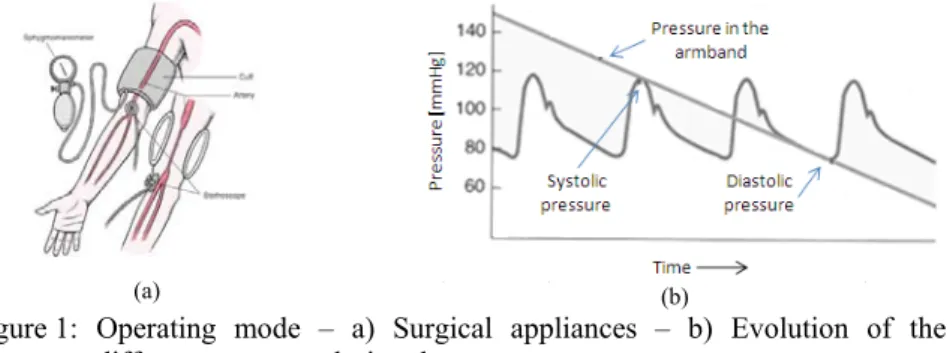
Figure 1: Operating mode – a) Surgical appliances – b) Evolution of the different pressures during the measurement

It requires the use of a sphygmomanometer (which is a control device of pressure composed of a manometer and a peer allowing the pressure to be induced), an armband and a stethoscope (cf. Figure 1-a). First, a pressure must be induced through the armband, in order to stop the blood flow. Then, by letting this pressure decreasing, the flow resumes and makes some noise called “Korotkoff’s noise”.

The doctor then supplies two numbers. The first one corresponds to the pressure when the flow begins (first noise) and the second one to the pressure when the flow stabilizes (no external effect anymore, the noise disappears gradually during the deflation and finally stop). They are respectively called the systolic and diastolic pressure (cf. Figure 1-b). A patient called physiologically normal shall have a pressure around [120, 80] mmHg, what the doctor will call 12/8.

The objective at the University of Liège has been to simulate this operating mode. With a numerical access to the phenomenon, one could avoid the problem of surgical appliances’ inaccuracy, and in this way find corrective factors to interpret the falsified measures.

2 Solution method

The goal intended is to simulate the discharge of the blood in the arteries, more particularly in the brachial artery during blood pressure measurement.

Ingeniously speaking, the artery can be modelled as a particular deformable pipe, when the blood is actually a fluid with specific properties. Thus the researches cover two complementary and interconnected domains, so be it the solid mechanics and the fluid mechanics, both studied at the MS²F sector.

With the solid mechanics, analytic relations between the external strains (not only the armband’s pressure, but also the blood pressure) and the deformations can be obtained, using either linear or non-linear theories. In this manner, the way the artery changes its shape may be determined. Given the mathematically known deformations for the artery, it remains to study the discharge of the blood in this particular deformable pipe, what has been done with specific original VisualBasic routines, but also with the modelling system WOLF from the HACH (Applied Hydrodynamics and Hydraulic Constructions), which is a finite volume flow simulation model developed at the University of Liège.

Figure 2: Scheme of the solution method

Behind these theoretical studies, bigger challenges arise. It effectively appears that while the medical understanding of the phenomenon is real, the knowledge of many factors is quite poor. Thus many elements, e.g. the boundary conditions or the mechanical parameters of the living tissues (depending on the chosen material model), have to be investigated using experiments. In this way, the authors have conducted a number of parallel researches about anatomical and physiological data, with the final purpose of completing and calibrating the models, but also to finally validate their accuracy.

3 Equations from Solid Mechanics Analysis

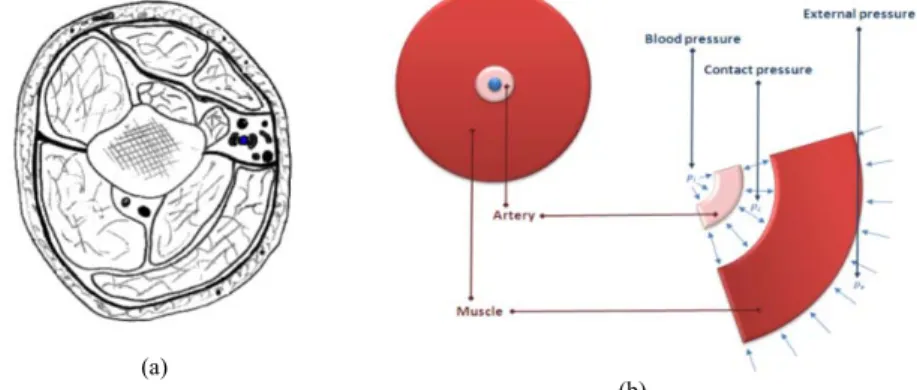
Under geometrical (cf. Figure 3) and phenomenological (the contact between the materials are assumed to be perfect) idealization, mathematical analysis have been performed in order to determine the way the artery deflates under specific strains (so be it the internal and external pressures). Thus the artery has been imagined as a particular pipe, and mathematical developments have been lead, to finally get analytic relations between the section and the pressures.

(a)

(b)

Figure 3: Transverse section of the arm – a) Actual situation – b) Idealized situation

To obtain the analytic results, two main hypotheses have to be made, one concerning the materials’ properties and the other the materials’ behaviour under strain; the muscle and the artery are supposed to be transversely isotropic and to follow a plane state of strain. These two assumptions come from observations about the materials’ structure, as seen in Figure 4, and are rather acceptable. In fact, the structures of both the artery and the muscle are concentric and present a cylindrical symmetry [1]. Moreover, the stresses are perpendicular to the solids’ generatrix, and one can reasonably accept that the distortions are nil in the longitudinal direction [1]. (a) (b)

Besides, the materials’ behaviour must also be assumed. In this way, it has been chosen to study the two materials from linear and non-linear perspectives. Despite the fact that the known response toward external strains follows non-linearity (because of the big deformations actually arising) the linear analysis can give a practical and prompt insight of the problem, and has thus been studied as well.

The linear analysis gives a first approach of the problem, and the different developments are rather obvious [1]. The results lied above and represent the radial displacement for the artery (eq.(1))

(

)

(

(

)

(

3 2

) (

)

2

)

1 2 2 1 1 1 1 1 2 2 x x r i i i c i c i c i c c i u r r r p r r p p p r r G r r ν ⎛ ⎞ = = ⎜_⎜ ⎟_⎟ − − + − − ⎝ ⎠ (1) ( ) ( ) ( )

(

)

(

( )

)

2 2 1 2 2 2 2 2 1 2 2 2 2 2 2 1 2 2 2 2 2 1 1 1 1 1 1 1 2 1 1 1 1 1 2 1 2 c i i e e c i e c x c e c i e c c i r p r p G r r G r r p r r r r G r r G r r ν ν ν ν ⎛ ⎞ ⎛ ⎞ − + − ⎜ ⎟ ⎜ ⎟ ⎜ ₋ ⎟ ⎜ ₋ ⎟ ⎝ ⎠ ⎝ ⎠ = ⎛ ⎛ ⎞ ⎛ ⎞ ⎞ ⎜ ⎜_⎜ ⎟_⎟ − + + ⎜_⎜ ⎟_⎟ − + ⎟ ⎜ _{⎝ − ⎠ ⎝ − ⎠} ⎟ ⎝ ⎠ (2)

Where ur [m] is the radial displacement, Gj [MPa] is the shear modulus of the materials, νj [-] is the Poisson coefficient of the materials, rk [m] is the radius of the zones, pk [Pa] is the pressure of the zones, pcx [Pa] is the equilibrium contact pressure, j = (1,2) = (artery,muscle), k = (i,c,e) = (artery,contact,muscle).

Similar results can be obtained for the non-linear analysis (see [1]). However, in order to physically interpret the results of the model in this second case, it would also be necessary to deeply investigate the non-linear parameters, which are for now almost absolutely unknown.

4 Specificities of Blood

The blood is actually a particular fluid. Before going further to the subject, it is form great importance to precise what makes it so specific. Its composition, of plasma and formed elements, lead its viscosity to be non-Newtonian. In fact, the presence of a solid part (the plasma) influences the behaviour of the fluid.

However, in large vessels, the fluid can be considered as Newtonian and homogeneous [3]-[4], as the boundary layer is very small compared to the vessel’s radius. In the capillaries, this assumption is no longer acceptable, the flow being determined mainly by viscous stresses.

Beside, one can reasonably assume that the blood is incompressible, the Mach number being globally quite small.

Finally, the turbulent effects have been neglected. It is well known that some source of instabilities create local turbulence, but analysis of both Reynolds and Womersley numbers show that this last hypothesis is acceptable [5].

For the smaller vessels, however, these assumptions have to be reconsidered, but for now, they have not been updated.

5 Mathematical Model

The equations of the every fluid mechanics problem are the Navier-Stokes equations (eq.(3)).

(

)

2 1 t U _{U U p U} t ρ ν ρ ∂Ω ⎧ _{+ ∇ ⋅Ω} ⎪ ∂ ⎪ ⎨∂ − ⎪ _{+ ⋅∇ = ⋅∇ + ⋅∇} ⎪ ∂ ⎩ (3) They represent respectively the conservation of the mass and the momentum.

The two variables are the section Ω and the velocity U. 5.1 Integration of the equations on the area

In the specific framework of blood discharge, some behavioural observations can be done. First, the flow is mostly one-dimensional. Second, the vertical accelerations are negligible, the pressure being thus hydrostatic. Finally, despite the fact that the streamline curvature can not actually be considered as small, no serious mistakes are made if these are neglected [5]. With these three acceptable assumptions in mind, the Navier-Stokes equations can be area-integrated [6] into the following form:

(

)

2 1 2 1 l x x l Q q t x Q Q gI gI F S Uq t x ϕ ρ ∂Ω ∂ ⎧ _{+ =} ⎪ ∂ ∂ ⎪ ⎨_{∂ ∂ ⎛ ⎞} ⎪ _{+ ⎜ + ⎟= + + +} ⎜ ⎟ ⎪ ∂ ∂ _⎝ Ω _⎠ ⎩ (4) With

( )

(

) ( )

( )

(

) ( )

1 2 , , ; f f b b h h h h l x I h h l x d I h h d x ξ ξ ξ ξ ξ ξ − − ∂ = − = − ∂

∫

∫

(5)

Where t [s] is the time, x [m] is the axial position, Ω [m²] is the section, Q [m³/s] is the discharge, ql [m²/s] is the lateral in- or out-flow, φ [-] is the parameter of non-uniform velocity repartition on the section, g [m/s²] is the gravity acceleration, ρ [kg/m³] is the density of blood, Sx [kg/s²] is the integrated effect of Reynolds axial stresses, Fx [kg/s²] is the global effect of roughness and U [m/s] is the axial velocity. One must keep in mind that this set of equation is valuable under the assumptions made about the blood in section 4.

5.2 The Preismann Slot

The presented equations are usually used to characterize free-surface flows. The Preismann Slot model [7] introduces an ingenious device to allow the modelling of both free surface and pressurized flows through the same set of equations. It consists in considering a narrow slot on the top of a closed pipe. The width of the slot (Tf [m]) is chosen in order to represent the behaviour of the conceptual free

surface flow, with a gravity wavespeed represented by f g c T Ω = (6).

6 Numerical Resolution

The set of equations introduced above (cf. section 5.1) requires the use of a

numerical resolution. As for most of the hydraulic problems, the finite volume method seems to be the most appropriate way to solve the problem. In this section, we will first present the algorithm itself. Second, the boundary conditions required will be discussed.

6.1 Algorithm

The set of equations can be written as follow

( )

( )

t x

∂ ₊ ∂ ₌

∂ U ∂ F U S U (7)

Where the vectors of conservative variables, flux and sources are respectively

( )

( )

₍

₎

2 1 ; _² ; 1 l x x l q Q Q _{gI S F Uq} Q ϕ gI _ρ ⎛ ⎞ ⎛ ⎞ Ω ⎛ ⎞ _{⎜ ⎟ ⎜ ⎟} =_{⎜ ⎟} = =_{⎜ ⎟} + + + ⎜ + ⎟ ⎝ ⎠ _{⎝ Ω ⎠} ⎜_⎝ ⎟_⎠ U F U S U (8)

Finally, the integration of (7) lead to the following conservative formulation:

1 1 1 i 2 i 2 n n i i t x + − + _{= − Δ} ⎡_⎢ − ⎤_⎥ ⎢ Δ ⎥ ⎣ ⎦ F F U U + S (9)

The numerical resolution uses a Runge-Kutta time-splitting scheme of the third order, with the three following sub-step evaluation

( )

( )

( )

( )

( )

( )

( )

( )

( )

1 1 ,1 2 2 ,1 ,1 1 1 ,2 2 2 ,1 ,2 ,2 1 1 ,3 2 2 ,2 n n i i i i n n n i i i n n i i i i n n n i i i n n i i i i n n n i i i t x t x t x + − + − + − ⎡ − ⎤ ⎢ ⎥ = − Δ _⎢ + _⎥ Δ ⎢ ⎥ ⎣ ⎦ ⎡ ₋ ⎤ ⎢ ⎥ = − Δ _⎢ + _⎥ Δ ⎢ ⎥ ⎣ ⎦ ⎡ ₋ ⎤ ⎢ ⎥ = − Δ _⎢ + _⎥ Δ ⎢ ⎥ ⎣ ⎦ F U F U U U S U F U F U U U S U F U F U U U S U (10)

And the final solution is given by

1 ,1 ,2 ,3 with 1 n n n n i α i β i γ i α β λ + _{= + +} + + = U U U U (11) 6.2 Boundary Conditions

The numerical resolution requires the imposition boundary conditions, actually one per each variable. The habit would be the forcing of the section and the

pressure, either at the downstream or the upstream. However, these quantities are not measurable; in fact, having access to such numerical values would require probing or in vivo tests, what is out of our skills.

(a) (b)

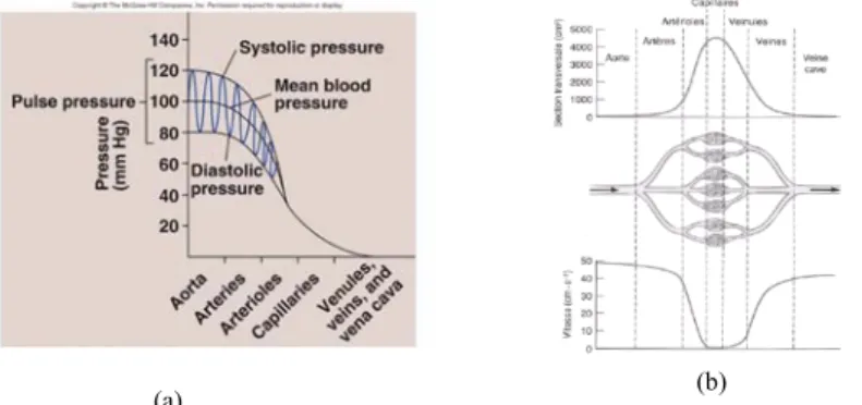
Figure 5: Evolution in the vessels – a) Systolic and diastolic pressures – b) Section and velocity

At the MS²F, the fact that the behaviour of both velocities and pressures are known in the capillaries (cf. Figure 5) has been used. The boundary conditions

are thus implemented as capillaries conditions, what can be done using branches following the architecture of vessels in the arm (cf. Figure 6-a and -b).

(a)

(b)

(c)

Figure 6: Architecture of the vessels – a) Transition between arteries and veins – b) Capillaries network – c) Simplified Capillaries network

7 Modelling

On one hand, the flow through the artery is modelled considering a single rectilinear pipe, with the only boundary condition being the upstream discharge. On the other hand, localized capillary-pumping (as shown on Figure 6) is considered such that the flow entering the micro-vascular network behaves as observed on Figure 5, so that its oscillation damped and the pressure decays. For now, the complete modelling (from the entrance of the artery to the exit after the multiple capillaries network) has not been done, but severe tests have been

performed in order to characterize the behaviour of both the artery and the capillaries network on their own.

For the final integration to be done, it remains to determine the pumping law, so the way the volume of blood is distributed from the artery to the smaller vessels as a function of the arterial pressure.

Moreover, the integration of the walls’ behaviour remains to be done. At the moment, the modelling of the blood discharge has been made with walls free of movement.

8 Results

As said before, the only results we have for now concern on one hand the mechanical behaviour of the vessels and on the other hand the hydraulic behaviour of both the artery and the capillaries network on their own. Those are successively introduced and examined in this section.

8.1 Behaviour of the materials

The established equations give the response of both the artery and the muscle to the external strains. Severe results and their analysis can be found in [1].

8.2 Modelling of the Artery

For the artery on its own, the numerical resolution needs to assume the downstream pressure, since the capillaries conditions have not been implemented yet. With a hypothetic constant pressure at the downstream and a periodic sinusoidal-type discharge at the upstream, the numerical model gives results similar to the one presented bellow (see Figure 7 & Figure 8).

The behaviour is typical for the described flow, whose regime is clearly subcritical.

Figure 8: Evolution of the heat [m] as a function of the time [s] for the downstream and the upstream

The presented results correspond to the following data: Lmax = 15m (length); Φmean = 0.25m (mean diameter for an empty slot); Δx = 0.1m; Nc = 0.1 (CFL number); Tf = 0.001m; fRoughness = 0.02; RK1 = 0.15; RK2 = 0.45; RK3 = 0.4; QUpstream,mean = 8m³/s. The fluid characteristics are the water’s one.

As it can be seen above, the parameters do not fit at all with the physiologic values that can be found in the literature. At this point of the researches, it has been chosen to analyse the problem with a qualitative point of view, in order to preserve the model from any scale problem.

8.3 Modelling of the Capillaries Network

For the modelling of the capillaries network, the resolution scheme seen in equations (7)-(11) must be reconsidered. The network is actually simplified as shown in Figure 6-c, and the model focus on only one path. There are thus no considerations of lateral outflow, but the junctions are taken into account by considering a revaluation of the incoming flux.

The goal of this modelling is to well represent the behaviour noticed in section 6.2. By choosing appropriate values for the roughness coefficient and the Preismann slot (values that are for now dictated only by a qualitative representation will) the dampening of the heat can be well represented. In fact, these two parameters are able to translate in a certain way how the surrounded materials behave.

Once again, a hypothetic constant pressure at the downstream and a periodic sinusoidal-type discharge at the upstream have been chosen. The numerical

model gives results similar to the one presented bellow (see Figure 9 & Figure 10).

The important point here is not the evolution in respect to the axial position, but rather the one with respect to the time (see Figure 10).

Figure 9: Evolution – a) of the discharge [m³/s] and – b) the heat [m] as a function of the axial position [m]

Figure 10: Evolution of the heat [m] as a function of the time [s] for the downstream and the upstream

It is effectively clear, by a comparison of these results and the one presented in section 8.2, that the consideration of a wide capillaries subdivision combined with appropriate parameters that represent the dissipative behaviour of the materials lead to the observation of the wanted dampening.

The presented results correspond to the following data: Lmax = 15m; Φmean = 0.25m; Δx = 0.025m; Nc = 0.1; Tf = 0.01m; fRoughness = 0.2; RK1 = 0.15; RK2 = 0.45; RK3 = 0.4; QUpstream,mean = 4m³/s; lcap = 0.5m (length of one intermediate segment). The fluid characteristics are once again the water’s one.

9 Conclusions

For now, the researches are still at their very beginning, and there are plenty of perspectives already in our mind. From the precision of the parameters to the final integration of the two presented models, the best is yet to come.

However, several interesting results have already been found, and allow us to think about the remaining work with confidence.

The reflexions about the boundary conditions have earned to be highlighted, the results presented in section 8.3 showing clearly the expected behaviour. Moreover, as the parameters have not been clarified at this time, it is expected that the quantitative aspect of this specificity will also be pointed as soon as this obstacle will be overcome.

Finally, on one hand the developed mechanical equations are ready to be implemented, while on the other hand the developed model has been elaborated such that the incoming modifications should be easy.

10 References

[1] Paulus, R. Analyse des effets mécaniques et hydrauliques induits dans le bras par un brassard de mesure de la pression artérielle. 2007. Master thesis,

University of Liège, Belgium.

[2] Paulus, R., B.J. Dewals, S. Erpicum, S. Cescotto, and M. Pirotton. Numerical

Analysis of Coupled Mechanical and Hydraulic Effects Induced by a Blood Pressure Meter. 2008. Proceedings of the 4th International Conference on

Advanced Computational Methods in Engineering (ACoMEn), Liège, Belgium. [3] Fung, Y.C. Biomechanics, Circulation. 1996. Springer Science, New York,

USA.

[4] Fung, Y.C. Biomechanics, Mechanical Properties of Living Tissues. 1993. Springer Science, New York, USA.

[5] Pochet, T. Ecoulement pulsatoire d’un fluide dans une conduite à parois

déformables. 1986. Master thesis, University of Liège, Belgium.

[6] Archambeau, P. Contribution à la modélisation de la genèse et de la

propagation des crues et innondations. 2006. Thesis, University of Liège,

Belgium.

[7] Preismann, A. Propagation des intumescences dans les canaux et rivières. First