Pépite | Réagir et s'adapter à son environnement : concevoir des méthodes autonomes pour l'optimisation combinatoire à plusieurs objectifs

Texte intégral

(1)Thèse de Aymeric Blot, Université de Lille, 2018. U NIVERSITÉ DE L ILLE – C RIStAL É COLE D OCTORALE S CIENCES P OUR L’I NGÉNIEUR. R EACTING AND A DAPTING TO THE E NVIRONMENT Designing Autonomous Methods for Multi-Objective Combinatorial Optimisation R ÉAGIR ET S ’ ADAPTER À SON ENVIRONNEMENT Concevoir des méthodes autonomes pour l’optimisation combinatoire à plusieurs objectifs B LOT Aymeric Thèse préparée et soutenue publiquement le 21 septembre 2018, en vue de l’obtention du grade de Docteur en Informatique. Jury: Mr. Mr. Mr. Mrs. Mrs. Mr. Mr. Mr.. B ATTITI Roberto D E C AUSMACKER Patrick H OOS H. Holger J OURDAN Laetitia K ESSACI Marie-Éléonore M ATHIEU Philippe S AUBION Frédéric S TÜTZLE Thomas. University of Trento KU Leuven Leiden University University of Lille University of Lille University of Lille University of Angers Université Libre de Bruxelles. Referee Examiner Examiner Supervisor Co-adviser Examiner Referee Examiner. Centre de Recherche en Informatique, Signal et Automatique de Lille Université Lille 1 – Bâtiment M3 extension – Avenue Carl Gauss 59655 Villeneuve d’Ascq Cedex FRANCE. © 2018 Tous droits réservés.. lilliad.univ-lille.fr.

(2) Thèse de Aymeric Blot, Université de Lille, 2018. © 2018 Tous droits réservés.. lilliad.univ-lille.fr.

(3) Thèse de Aymeric Blot, Université de Lille, 2018. Acknowledgements First of all I would like to thank the jury members and especially Laetitia Jourdan and Marie-Éléonore Kessaci, that supported me during the last three years on an every-day basis. Laetitia, I am very grateful for everything you have done since I met you for the first time six years ago, in particular for the many research opportunities in Lille but also in Nagano and in Vancouver. Marie-Éléonore, you taught me perseverance and thoroughness; without your advising this thesis would definitively not have happened. Many thanks to Patrick de Causmaecker, Philippe Mathieu, and Thomas Stützle for accepting to be part of my jury, and to Roberto Battiti and Frederic Saubion for also reporting on my manuscript; I am honoured for the interest you gave to my work. I would like to thank my coauthors Patrick de Causmaecker, Holger H. Hoos, Manuel López-Ibáñez, and Heike Trautmann, for the work we carried out together during this thesis. Our discussions have brought so much and pushed this thesis much further than I could have done by myself. I also want to thank Hernán Aguirre and Kiyoshi Tanaka: I only stayed in Nagano three months but I will never forget them; they confirmed my passion for research and changed my life forever. どうもありがとうございました。 Generally speaking, thank you everyone from the ORKAD team, the former DOLPHIN team, and my colleagues from INRIA and the CRIStAL laboratory. I will also always keep very good memories from the years I spent at the ENS Rennes: they brought me my passion for computer science and research, and I could not have dreamt for a better formation. I cannot thank enough the friends I made along the way, in Orsay, in Rennes, and in Lille. Thank you Grégoire, Thomas, Hugo, Nicolas, Lauriane, Mathieu, Lucien, Maxence, and Léonard; I was not always easy to put up with, but you supported me and I would not be where I stand today without you. Finally, I am grateful to my family. To my parents, for their constant support during the last 26 years; and to my brother and sister and their companions for giving me three wonderful nieces.. i. © 2018 Tous droits réservés.. lilliad.univ-lille.fr.

(4) Thèse de Aymeric Blot, Université de Lille, 2018. ii. © 2018 Tous droits réservés.. Acknowledgements. lilliad.univ-lille.fr.

(5) Thèse de Aymeric Blot, Université de Lille, 2018. Contents General Introduction. 1. Motivations . . . . . . . . . . . . . . . . . . . . . . . . . . . . . . . . . . . . Outline . . . . . . . . . . . . . . . . . . . . . . . . . . . . . . . . . . . . . . .. 1 3. I. Multi-objective Optimisation and Algorithm Design. 7. 1. Multi-objective Metaheuristics 1.1 Multi-objective Combinatorial Optimisation . . . . 1.1.1 Introduction . . . . . . . . . . . . . . . . . . . 1.1.2 Definition . . . . . . . . . . . . . . . . . . . . 1.1.3 Solution Comparison . . . . . . . . . . . . . . 1.1.4 Multi-objective Metaheuristics . . . . . . . . 1.2 Performance Assessment . . . . . . . . . . . . . . . . 1.2.1 Overview . . . . . . . . . . . . . . . . . . . . 1.2.2 Hypervolume . . . . . . . . . . . . . . . . . . 1.2.3 ∆ Spread . . . . . . . . . . . . . . . . . . . . . 1.3 Permutation Problems . . . . . . . . . . . . . . . . . 1.3.1 Permutation Flow Shop Scheduling Problem 1.3.2 Travelling Salesman Problem . . . . . . . . . 1.3.3 Quadratic Assignment Problem . . . . . . .. 2. . . . . . . . . . . . . .. Automatic Algorithm Design 2.1 Preliminaries . . . . . . . . . . . . . . . . . . . . . . . . 2.2 Overview . . . . . . . . . . . . . . . . . . . . . . . . . . 2.2.1 Algorithm Selection . . . . . . . . . . . . . . . 2.2.2 Algorithm Configuration / Parameter Tuning 2.2.3 Parameter Control . . . . . . . . . . . . . . . . 2.2.4 Hyper-heuristics . . . . . . . . . . . . . . . . . 2.2.5 Other Fields and Taxonomies . . . . . . . . . . 2.2.6 Multi-objective Automatic Design . . . . . . .. . . . . . . . . . . . . .. . . . . . . . .. . . . . . . . . . . . . .. . . . . . . . .. . . . . . . . . . . . . .. . . . . . . . .. . . . . . . . . . . . . .. . . . . . . . .. . . . . . . . . . . . . .. . . . . . . . .. . . . . . . . . . . . . .. . . . . . . . .. . . . . . . . . . . . . .. . . . . . . . .. . . . . . . . . . . . . .. . . . . . . . .. . . . . . . . . . . . . .. 9 9 9 10 10 12 14 14 15 16 17 17 19 21. . . . . . . . .. 23 24 25 26 27 29 30 31 32. iii. © 2018 Tous droits réservés.. lilliad.univ-lille.fr.

(6) Thèse de Aymeric Blot, Université de Lille, 2018. iv. Contents 2.3. II 3. 4. © 2018 Tous droits réservés.. Overall Automatic Design Taxonomy Proposition 2.3.1 Temporal Viewpoint . . . . . . . . . . . . . 2.3.2 Structural Viewpoint . . . . . . . . . . . . . 2.3.3 Overview . . . . . . . . . . . . . . . . . . . 2.3.4 Additional Complexity Viewpoint . . . . .. . . . . .. . . . . .. . . . . .. . . . . .. . . . . .. . . . . .. . . . . .. . . . . .. . . . . .. . . . . .. . . . . .. Multi-objective Local Search. 39. Unified MOLS Structure 3.1 Preliminaries . . . . . . . . . . . . . . . . . . . . . . . . . . . 3.1.1 Definitions . . . . . . . . . . . . . . . . . . . . . . . . 3.1.2 Historical Development . . . . . . . . . . . . . . . . 3.1.3 Condensed Literature Summary . . . . . . . . . . . 3.1.4 Analysis and Discussion . . . . . . . . . . . . . . . . 3.2 MOLS Strategies . . . . . . . . . . . . . . . . . . . . . . . . . 3.2.1 Set of Potential Pareto Optimal Solutions (Archive) 3.2.2 Set of Current Solutions (Memory) . . . . . . . . . . 3.2.3 Exploration Strategies . . . . . . . . . . . . . . . . . 3.2.4 Selection Strategies . . . . . . . . . . . . . . . . . . . 3.2.5 Termination Criteria . . . . . . . . . . . . . . . . . . 3.3 Escaping Local Optima . . . . . . . . . . . . . . . . . . . . . 3.4 MOLS Unification Proposition . . . . . . . . . . . . . . . . . 3.4.1 Main Loop . . . . . . . . . . . . . . . . . . . . . . . . 3.4.2 Local Search Exploration . . . . . . . . . . . . . . . 3.4.3 Iterated Local Search Algorithm . . . . . . . . . . . 3.5 Literature Instantiation . . . . . . . . . . . . . . . . . . . . . MOLS Instantiations 4.1 Static MOLS Algorithm . . . . . . 4.1.1 Algorithm . . . . . . . . . 4.1.2 Configuration Space . . . 4.2 Control Mechanisms Integration 4.2.1 Parameter Analysis . . . . 4.2.2 Knowledge Exploitation . 4.2.3 Knowledge Extraction . . 4.2.4 Knowledge Modelling . . 4.2.5 Decisional Schedule . . . 4.3 Adaptive MOLS Algorithm . . . 4.3.1 Algorithm . . . . . . . . .. 32 32 33 35 37. . . . . . . . . . . .. . . . . . . . . . . .. . . . . . . . . . . .. . . . . . . . . . . .. . . . . . . . . . . .. . . . . . . . . . . .. . . . . . . . . . . .. . . . . . . . . . . .. . . . . . . . . . . .. . . . . . . . . . . .. . . . . . . . . . . .. . . . . . . . . . . .. . . . . . . . . . . .. . . . . . . . . . . .. . . . . . . . . . . .. . . . . . . . . . . . . . . . . .. . . . . . . . . . . .. . . . . . . . . . . . . . . . . .. . . . . . . . . . . .. . . . . . . . . . . . . . . . . .. . . . . . . . . . . .. . . . . . . . . . . . . . . . . .. . . . . . . . . . . .. . . . . . . . . . . . . . . . . .. . . . . . . . . . . .. . . . . . . . . . . . . . . . . .. 41 41 41 43 49 51 52 52 53 53 56 56 56 57 57 58 59 59. . . . . . . . . . . .. 63 64 64 66 68 68 69 69 70 70 72 72. lilliad.univ-lille.fr.

(7) Thèse de Aymeric Blot, Université de Lille, 2018. Contents. 4.4. 4.5. 4.6. III 5. 6. 4.3.2 Related adaptive MOLS Algorithms Configuration Scheduling . . . . . . . . . . 4.4.1 Proposition . . . . . . . . . . . . . . 4.4.2 Definitions . . . . . . . . . . . . . . . 4.4.3 Related Approaches . . . . . . . . . AMH: Adaptive MetaHeuristics . . . . . . 4.5.1 Motivation . . . . . . . . . . . . . . . 4.5.2 Philosophy . . . . . . . . . . . . . . 4.5.3 Design and Implementation . . . . . 4.5.4 Execution Flow Examples . . . . . . Perspectives . . . . . . . . . . . . . . . . . .. v . . . . . . . . . . .. . . . . . . . . . . .. . . . . . . . . . . .. . . . . . . . . . . .. . . . . . . . . . . .. . . . . . . . . . . .. . . . . . . . . . . .. . . . . . . . . . . .. . . . . . . . . . . .. . . . . . . . . . . .. . . . . . . . . . . .. . . . . . . . . . . .. . . . . . . . . . . .. . . . . . . . . . . .. . . . . . . . . . . .. Automatic Offline Design MO-ParamILS 5.1 Multi-objective Automatic Configuration . . . . . . . . 5.1.1 Definition . . . . . . . . . . . . . . . . . . . . . . 5.1.2 Use Cases . . . . . . . . . . . . . . . . . . . . . . 5.2 Single-objective ParamILS . . . . . . . . . . . . . . . . . 5.2.1 Core Algorithm . . . . . . . . . . . . . . . . . . . 5.2.2 BasicILS, FocusedILS . . . . . . . . . . . . . . . . 5.2.3 Adaptive Capping Strategies . . . . . . . . . . . 5.2.4 Configuration Protocol . . . . . . . . . . . . . . . 5.3 Multi-objective ParamILS . . . . . . . . . . . . . . . . . 5.3.1 Motivations . . . . . . . . . . . . . . . . . . . . . 5.3.2 Core Algorithm . . . . . . . . . . . . . . . . . . . 5.3.3 Configuration Protocol . . . . . . . . . . . . . . . 5.4 Hybrid Multi-Objective Approaches . . . . . . . . . . . 5.4.1 Single Performance Indicator . . . . . . . . . . . 5.4.2 Aggregation of Multiple Performance Indicators 5.5 Framework Evaluation . . . . . . . . . . . . . . . . . . . 5.5.1 Experimental Protocol . . . . . . . . . . . . . . . 5.5.2 Results . . . . . . . . . . . . . . . . . . . . . . . . 5.6 Perspectives . . . . . . . . . . . . . . . . . . . . . . . . .. 72 74 75 75 76 77 77 78 79 80 80. 85 . . . . . . . . . . . . . . . . . . .. . . . . . . . . . . . . . . . . . . .. . . . . . . . . . . . . . . . . . . .. . . . . . . . . . . . . . . . . . . .. . . . . . . . . . . . . . . . . . . .. . . . . . . . . . . . . . . . . . . .. . . . . . . . . . . . . . . . . . . .. . . . . . . . . . . . . . . . . . . .. 87 87 87 88 89 89 93 94 96 97 97 98 102 102 102 103 103 104 106 111. MOLS Configuration 113 6.1 Exhaustive Analysis . . . . . . . . . . . . . . . . . . . . . . . . . . . . 114 6.1.1 Experimental Protocol . . . . . . . . . . . . . . . . . . . . . . . 114 6.1.2 Parameter Distribution Analysis . . . . . . . . . . . . . . . . . 117. © 2018 Tous droits réservés.. lilliad.univ-lille.fr.

(8) Thèse de Aymeric Blot, Université de Lille, 2018. vi. Contents. 6.2. 6.3. 6.4. IV 7. © 2018 Tous droits réservés.. Optimal Configurations . . . . . . . . . . . . . . . . . . . . . . 117. 6.1.4. Discussions . . . . . . . . . . . . . . . . . . . . . . . . . . . . . 119. AAC Approaches Analysis . . . . . . . . . . . . . . . . . . . . . . . . . 122 6.2.1. Experimental Protocol . . . . . . . . . . . . . . . . . . . . . . . 122. 6.2.2. Small Configuration Space Results . . . . . . . . . . . . . . . . 124. 6.2.3. Large Configuration Space Results . . . . . . . . . . . . . . . . 128. 6.2.4. Discussions . . . . . . . . . . . . . . . . . . . . . . . . . . . . . 130. Analysis of Objective Correlation . . . . . . . . . . . . . . . . . . . . . 131 6.3.1. Experimental Protocol . . . . . . . . . . . . . . . . . . . . . . . 131. 6.3.2. Optimised Configurations . . . . . . . . . . . . . . . . . . . . . 133. 6.3.3. Discussions . . . . . . . . . . . . . . . . . . . . . . . . . . . . . 138. Perspectives . . . . . . . . . . . . . . . . . . . . . . . . . . . . . . . . . 144. Automatic Online Design MOLS Control 7.1. 8. 6.1.3. 147 149. Adaptive MOLS Algorithm . . . . . . . . . . . . . . . . . . . . . . . . 150 7.1.1. Adaptive Algorithm . . . . . . . . . . . . . . . . . . . . . . . . 150. 7.1.2. Generic Online Mechanisms . . . . . . . . . . . . . . . . . . . . 151. 7.2. Experimental Protocol . . . . . . . . . . . . . . . . . . . . . . . . . . . 156. 7.3. Experimental Results . . . . . . . . . . . . . . . . . . . . . . . . . . . . 157 7.3.1. 3-arm Results . . . . . . . . . . . . . . . . . . . . . . . . . . . . 158. 7.3.2. 2-arm Results . . . . . . . . . . . . . . . . . . . . . . . . . . . . 158. 7.3.3. Long Term Learning Results . . . . . . . . . . . . . . . . . . . 159. 7.4. Discussions . . . . . . . . . . . . . . . . . . . . . . . . . . . . . . . . . 159. 7.5. Perspectives . . . . . . . . . . . . . . . . . . . . . . . . . . . . . . . . . 161. MOLS Configuration Scheduling. 163. 8.1. MOLS Configurations . . . . . . . . . . . . . . . . . . . . . . . . . . . 164. 8.2. Experimental Protocol . . . . . . . . . . . . . . . . . . . . . . . . . . . 165. 8.3. Experimental Results . . . . . . . . . . . . . . . . . . . . . . . . . . . . 166 8.3.1. Exhaustive Enumeration . . . . . . . . . . . . . . . . . . . . . . 167. 8.3.2. K = 2 Configuration Schedules . . . . . . . . . . . . . . . . . . 169. 8.3.3. K = 3 Configuration Schedules . . . . . . . . . . . . . . . . . . 172. 8.4. Discussions . . . . . . . . . . . . . . . . . . . . . . . . . . . . . . . . . 174. 8.5. Perspectives . . . . . . . . . . . . . . . . . . . . . . . . . . . . . . . . . 177. lilliad.univ-lille.fr.

(9) Thèse de Aymeric Blot, Université de Lille, 2018. Contents. General Conclusion. vii. 179. Contribution Summary . . . . . . . . . . . . . . . . . . . . . . . . . . . . . . 179 Future Research . . . . . . . . . . . . . . . . . . . . . . . . . . . . . . . . . . 182. Publications. 185. Bibliography. 187. © 2018 Tous droits réservés.. lilliad.univ-lille.fr.

(10) Thèse de Aymeric Blot, Université de Lille, 2018. viii. © 2018 Tous droits réservés.. Contents. lilliad.univ-lille.fr.

(11) Thèse de Aymeric Blot, Université de Lille, 2018. List of Figures 1.1 1.2 1.3 1.4 1.5 1.6 1.7. Normalised unary hypervolume indicator Normalised ∆ and ∆ ′ spread indicators . Example of PFSP schedule . . . . . . . . . Common PFSP schedule operations . . . Example of TSP tour . . . . . . . . . . . . Example of 2-opt recombination . . . . . Examples of QAP pairings . . . . . . . . .. . . . . . . .. . . . . . . .. . . . . . . .. . . . . . . .. . . . . . . .. . . . . . . .. . . . . . . .. . . . . . . .. . . . . . . .. . . . . . . .. . . . . . . .. . . . . . . .. . . . . . . .. . . . . . . .. . . . . . . .. . . . . . . .. 16 16 18 19 20 21 22. 2.1 2.2 2.3 2.4. Eiben et al. (1999) parameter setting taxonomy Algorithm selection general workflow . . . . . Algorithm configuration general workflow . . Algorithm design overview . . . . . . . . . . .. . . . .. . . . .. . . . .. . . . .. . . . .. . . . .. . . . .. . . . .. . . . .. . . . .. . . . .. . . . .. . . . .. 25 27 28 35. 3.1. Objective space with and without taking into account surrounding solutions . . . . . . . . . . . . . . . . . . . . . . . . . . . . . . . . . . . 55. 4.1 4.2 4.3 4.4 4.5 4.6 4.7 4.8 4.9. Inner MOLS loop . . . . . . . . . . . . . . . . . . . . . . . . . . Outer MOLS loop . . . . . . . . . . . . . . . . . . . . . . . . . . Control integration in the inner MOLS loop . . . . . . . . . . . Control integration in the outer MOLS loop . . . . . . . . . . . Examples of two configuration schedules . . . . . . . . . . . . Execution flow of an iterated MOLS algorithm . . . . . . . . . Execution flow of an adaptive algorithm using multiple paths Execution flow of an adaptive algorithm using reconstruction MOLS schedule . . . . . . . . . . . . . . . . . . . . . . . . . . .. . . . . . . . . .. . . . . . . . . .. . . . . . . . . .. . . . . . . . . .. 66 66 71 72 76 78 81 82 82. 5.1 5.2 5.3 5.4 5.5. Final fronts on the Regions200 – CPLEX (cutoff) scenario . . . . Final fronts on the Regions200 – CPLEX (running time) scenario Final fronts on the CORLAT – CPLEX (cutoff) scenario . . . . . Final fronts on the CORLAT – CPLEX (running time) scenario . Final fronts on the QUEENS – CLASP scenario . . . . . . . . . .. . . . . .. . . . . .. . . . . .. 107 107 108 108 109. ix. © 2018 Tous droits réservés.. lilliad.univ-lille.fr.

(12) Thèse de Aymeric Blot, Université de Lille, 2018. x. © 2018 Tous droits réservés.. List of Figures 6.1 6.2 6.3 6.4. Exhaustive analysis parameter distribution on test instances . . Experiments on the small configuration space – PFSP scenarios Experiments on the small configuration space – TSP scenarios . Experiments on the large configuration space . . . . . . . . . . .. . . . .. . . . .. . . . .. 118 126 127 129. 8.1 8.2 8.3 8.4 8.5. The seven types of schedules used in the experiments . Initial search space and optimal configurations (K = 1) Final optimised configuration schedules (K = 2) . . . . Final optimised configuration schedules (K = 3) . . . . Final comparison . . . . . . . . . . . . . . . . . . . . . .. . . . . .. . . . . .. . . . . .. 165 167 170 172 176. . . . . .. . . . . .. . . . . .. . . . . .. . . . . .. lilliad.univ-lille.fr.

(13) Thèse de Aymeric Blot, Université de Lille, 2018. List of Tables 3.1 3.2 3.3. Condensed literature summary . . . . . . . . . . . . . . . . . . . . . . 50 Condensed literature instantiation (LS Procedure) . . . . . . . . . . . 61 Condensed literature instantiation (EXPLORE Procedure) . . . . . . . 62. 4.1. Considered parameter space . . . . . . . . . . . . . . . . . . . . . . . . 67. 5.1 5.2 5.3. Configuration scenarios . . . . . . . . . . . . . . . . . . . . . . . . . Target algorithm parameters (with number of possible values) . . . Hypervolume (top) and ε indicator values (bottom) for final test fronts. . . . . . . . . . . . . . . . . . . . . . . . . . . . . . . . . . . . . Average percentages of timeouts for final CPLEX configurations . .. 5.4 6.1 6.2 6.3 6.4 6.5 6.6 6.7 6.8 6.8 6.9 6.9 6.10 6.11 6.12 6.13 6.14. Small version of the MOLS configuration space . . . . . . . . . . . . PFSP (optimal configurations) . . . . . . . . . . . . . . . . . . . . . . . TSP (optimal configurations) . . . . . . . . . . . . . . . . . . . . . . . . Large version of the MOLS configuration space . . . . . . . . . . . . AAC Experimental Protocol . . . . . . . . . . . . . . . . . . . . . . . Indicator bounds used in the HV+∆ ′ approach . . . . . . . . . . . . Number of configurations after training, validation and testing . . PFSP 50 jobs 20 machines (optimised configurations) . . . . . . . . . . PFSP 50 jobs 20 machines (optimised configurations, continued) . . . . PFSP 100 jobs 20 machines (optimised configurations) . . . . . . . . . PFSP 100 jobs 20 machines (optimised configurations, continued) . . . TSP 50 cities (optimised configurations) . . . . . . . . . . . . . . . . . . TSP 100 cities (optimised configurations) . . . . . . . . . . . . . . . . . QAP 50 facilities (optimised configurations) . . . . . . . . . . . . . . . QAP 100 facilities (optimised configurations) . . . . . . . . . . . . . . AAC performance: number of final configurations and objective ranges . . . . . . . . . . . . . . . . . . . . . . . . . . . . . . . . . . . . 6.14 AAC performance: number of final configurations and objective ranges (continued) . . . . . . . . . . . . . . . . . . . . . . . . . . . .. . 104 . 105 . 106 . 109 . . . . . . . . . . . . . . .. 115 120 121 123 124 125 130 134 135 136 137 139 140 141 142. . 143 . 144. xi. © 2018 Tous droits réservés.. lilliad.univ-lille.fr.

(14) Thèse de Aymeric Blot, Université de Lille, 2018. xii. List of Tables 7.1 7.2 7.3 7.4 7.5. Experiments summary . . . 3-arm ranking . . . . . . . . 2-arm ranking . . . . . . . . Long-time learning ranking Complete ranking . . . . . .. 8.1 8.2 8.3 8.4 8.5 8.6 8.7 8.7. Investigated MOLS configuration space . . . . . . . . . . . . . Training computational time . . . . . . . . . . . . . . . . . . . . Optimal configurations (K = 1) . . . . . . . . . . . . . . . . . . Optimal configurations (K = 1) . . . . . . . . . . . . . . . . . . Final optimised configuration schedules (K = 2; PFSP 20 jobs) Final optimised configuration schedules (K = 2; PFSP 50 jobs) Final optimised configuration schedules (K = 3; PFSP 20 jobs) Final optimised configuration schedules (K = 3; PFSP 20 jobs; tinued) . . . . . . . . . . . . . . . . . . . . . . . . . . . . . . . . Final optimised configuration schedules (K = 3; PFSP 50 jobs). 8.8. © 2018 Tous droits réservés.. . . . . .. . . . . .. . . . . .. . . . . .. . . . . .. . . . . .. . . . . .. . . . . .. . . . . .. . . . . .. . . . . .. . . . . .. . . . . .. . . . . .. . . . . .. . . . . .. . . . . .. . . . . .. . . . . .. . . . . .. . . . . .. . . . . .. . . . . .. . . . . .. 157 158 159 160 160. . . . . . . . . . . . . . . . . . . . . . con. . . . . .. . . . . . . .. 164 166 168 169 170 171 173. . 174 . 175. lilliad.univ-lille.fr.

(15) Thèse de Aymeric Blot, Université de Lille, 2018. List of Algorithms 3.1 3.2 3.3. Procedure LS(memory, archive) . . . . . . . . . . . . . . . . . . . . . 57 Procedure EXPLORE(current, ref, archive) . . . . . . . . . . . . . 58 Procedure ITER(archive) . . . . . . . . . . . . . . . . . . . . . . . . . 59. 4.1 4.2 4.3. Static Iterated Multi-Objective Local Search . . . . . . . . . . . . . . . . 65 Adaptive Iterated Multi-Objective Local Search . . . . . . . . . . . . . 73 Inner Multi-Objective Local Search (mols) . . . . . . . . . . . . . . . . 74. 5.1 5.2 5.3 5.4 5.5 5.6 5.7 5.8 5.9. Single-objective ParamILS . . . . . . . . Procedure localsearch(config) . . . . . . Procedure compare(config, challenger) Procedure update(config, reference) . . Procedure update(config, reference) . . Procedure intensify(config) . . . . . . . Multi-objective ParamILS . . . . . . . . Procedure localSearch(init_arch) . . . . Function archive(arch, challenger) . . .. . . . . . . . . .. . . . . . . . . .. . . . . . . . . .. . . . . . . . . .. . . . . . . . . .. . . . . . . . . .. . . . . . . . . .. . . . . . . . . .. . . . . . . . . .. . . . . . . . . .. . . . . . . . . .. . . . . . . . . .. . . . . . . . . .. . . . . . . . . .. . . . . . . . . .. . . . . . . . . .. . . . . . . . . .. . . . . . . . . .. 90 91 93 93 95 96 99 100 101. xiii. © 2018 Tous droits réservés.. lilliad.univ-lille.fr.

(16) Thèse de Aymeric Blot, Université de Lille, 2018. xiv. © 2018 Tous droits réservés.. List of Algorithms. lilliad.univ-lille.fr.

(17) Thèse de Aymeric Blot, Université de Lille, 2018. General Introduction The journey of a thousand miles begins with a single step. Lao-Tzu. This thesis lays on the intersections between multi-objective combinatorial optimisation, local search algorithms, and automatic algorithm design. It was carried out in the ORKAD1 team, that focuses on combining combinatorial optimisation and data mining to solve optimisation problems. Before its creation in 2017 as an independent research team in the CRIStAL2 laboratory, the ORKAD team was a research group associated to the DOLPHIN3 joint project team, collaboration between the CRIStAL laboratory and the Inria Lille-Nord Europe research institute.. Motivations Optimisation problems are ubiquitous. Numerous real-world problems, such as planning schedules, building financial portfolios, routing vehicles, or predicting future patients at risk in healthcare, can be formulated by determining the best solution among a very large number of possible ones. For many optimisation problems, while evaluating the quality of a single solution is usually fairly easy and quick, solving them to optimality is much more computationally expensive as their difficulty increases at least exponentially with the size of the problem. The question of whether of not these problems, called NP-hard, can theoretically be solved efficiently is at the core of one of the major unsolved problem of computer science: the P versus NP problem. In order to obtain good solutions for NP-hard problems that would be too large to be solved to optimality in reasonable time, or in general for any large-scale op1. Operational Research, Knowledge And Data Centre de Recherche en Informatique, Signal et Automatique de Lille (UMR CNRS 9189) 3 Discrete multiobjective Optimization for Large-scale Problems with Hybrid dIstributed techNiques 2. 1. © 2018 Tous droits réservés.. lilliad.univ-lille.fr.

(18) Thèse de Aymeric Blot, Université de Lille, 2018. 2. General Introduction. timisation problem, approximation algorithms such as metaheuristics have been proposed and are usually preferred. Local search algorithms are metaheuristics that focus on the structure of the problem to solve, in order to benefit from the relation between similar solutions and progressively and iteratively approach optimal solutions. They have been shown to be very efficient, either used as self-contained algorithms or hybridised into more complex metaheuristics. Along with the other metaheuristics, local search algorithms are very generic approaches that can be applied to many combinatorial optimisation problems as long as few assumptions over the problem modelling are respected, such as a finite or at least countable number of solutions. However, it is to be expected that no single algorithm can perform the best on every problem, so metaheuristics usually involves many possible variants, using many alternative strategies, to improve performance on specific problems structures. Given a specific problem, automatically determining which of the many variants of the algorithm will be the most efficient, or, more broadly, automatically designing the optimal algorithm that use the most efficient strategies, is a recent but thriving research field. Finally, optimisation problems as well as automatic design problems can involve more than a single criteria to optimise. If as single quality is to be maximised, or a single cost is to be minimised, the resolution process usually results in a single final optimal solution. However, considering multiple objectives usually involves a much richer context in which many incomparable compromise solutions are to be sought. If classical multi-objective optimisation problems are increasingly studied and understood, multi-objective concepts for algorithm design problems have only been considered recently.. Based on these observations, we investigate in this thesis the different intersections between combinatorial optimisation, local search algorithms, and automatic algorithm design, in the context of multi-objective optimisation. In particular, our focus is divided in one hand on multi-objective automatic algorithm design, i.e., the automatic design of algorithms relatively to multiple performance metrics, and on the other hand on the automatic design of multi-objective algorithms, using multi-objective local search algorithms. Finally, we investigate two aspects of adaptation using automatic algorithm design: first with a predictive viewpoint, where algorithms are configured with regard to performance on learning instances, and with an complementary adaptive viewpoint, where algorithms autonomously react during their execution to the instance being solved.. © 2018 Tous droits réservés.. lilliad.univ-lille.fr.

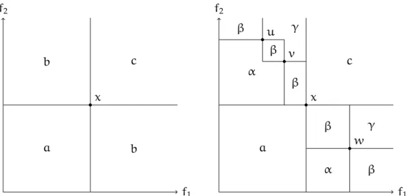
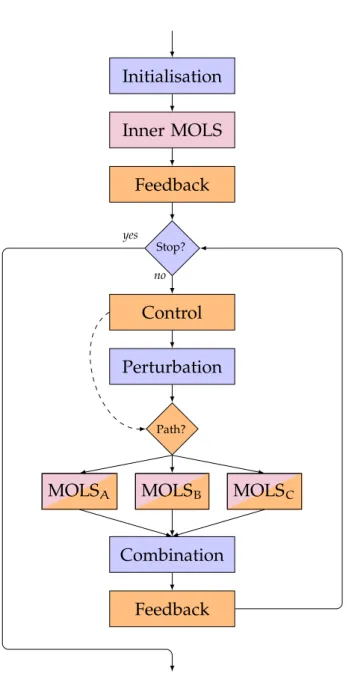
(19) Thèse de Aymeric Blot, Université de Lille, 2018. Outline. 3. Outline Following this general introduction, this thesis is organised in four successive parts, starting from general notions about multi-objective optimisation and presenting the state of the art of automatic algorithm design, then focusing on multiobjective local search (MOLS) algorithms, before focusing on automatically designing MOLS algorithms using offline algorithm design, and finally discussing two possible online extensions. Part I: Multi-objective Optimisation and Algorithm Design First, Part I lays the foundations of this thesis down, and presents the research fields of both combinatorial optimisation and algorithm design. Chapter 1 details the multi-objective context that we use in this thesis. We give the general definitions and notions of multi-objective combinatorial optimisation, we discuss the performance assessment of multi-objective algorithms, and we present the three combinatorial problems that will be tackled in the experiments of Part III and Part IV. Chapter 2 presents the research field of automatic algorithm design (AAD) with a proposition of a new taxonomy. We first introduce the foundations of our proposition, then we give a detailed overview of the existing related research fields and state of the art methods. Finally we present and motivate our taxonomy proposition by discussing existing works according to several general viewpoints: a temporal viewpoint: “when does the automatic design take place?”, a structural viewpoint: “how much of the algorithmic design can be modified?”, and finally a complementary complexity viewpoint, related to the available knowledge sources. Part II: Multi-objective Local Search Next, Part II focuses on the class of algorithms studied in this thesis, the multiobjective local search (MOLS) algorithms. Chapter 3 provides a technical and historical background on MOLS algorithms. We first present their specific notions and philosophy, and conduct a chronological survey of the use of local search techniques in multi-objective algorithms. Then, we discuss the local search strategies found in the literature, and finally we propose a new unification of MOLS algorithms and detail how the major literature algorithms are instantiated. Chapter 4 details the specific implementations of the MOLS algorithms that will be used in the following chapters, based on the unified structure presented in. © 2018 Tous droits réservés.. lilliad.univ-lille.fr.

(20) Thèse de Aymeric Blot, Université de Lille, 2018. 4. General Introduction Chapter 3. We first present a classical MOLS algorithm that exposes many parameters in order to automatically configure it in Chapter 6. Then, we discuss how we can involve generic mechanisms to dynamically control the value of some parameters of MOLS algorithms during their execution, and present the adaptive MOLS algorithm that is considered in Chapter 7. Finally, we present the notion of configuration scheduling that is investigated in Chapter 8.. Part III: Automatic Offline Design Then, Part III investigates offline AAD approaches, and more specifically multiobjective algorithm configuration, when the algorithm configuration is optimised before its execution. Chapter 5 introduces MO-ParamILS, a multi-objective automatic configuration framework based on MOLS techniques, as a dedicated approach for multiobjective configuration scenarios. First we formally define multi-objective algorithm configuration and detail some use cases. Then, we present ParamILS, a prominent and well-known single-objective algorithm configurator based on a single-objective local search, before proposing MO-ParamILS, that we based on a MOLS algorithm. Finally, we study the performance of the multiple variants of MO-ParamILS against approaches directly using ParamILS only on various use cases, to show the worth of using multi-objective approaches against classical single-objective approaches. Chapter 6 deals with the automatic design of MOLS algorithms. In the course of three successive studies, the use of a multi-objective configurator is compared against the use a single-objective configurator. Three configuration approaches are compared: first a classical baseline of optimising the convergence of the MOLS algorithms, then an aggregated approach focusing on convergence while taking into account the distribution of solutions, and finally the simultaneous optimisation of both convergence and distribution independently. The first study provides comprehensive preliminary results on classical problems by limiting itself to a small subset of possible MOLS configurations. The second study provides conclusive results by tackling a much larger pool of configuration. Finally the third study validates our observations by tacking artificially constructed scenarios on which the correlation between objectives is controlled. To ensure fair comparisons, the multi-objective and singleobjective approaches used are based on ParamILS and MO-ParamILS, as they are based on the same principles.. © 2018 Tous droits réservés.. lilliad.univ-lille.fr.

(21) Thèse de Aymeric Blot, Université de Lille, 2018. Outline. 5. Part IV: Automatic Online Design Last, Part IV discusses two extensions of MOLS automatic design, involving online elements, i.e., when modifications of the MOLS configuration occur during the execution. Chapter 7 uses notions of parameter control to delay the prediction of the optimal configuration. Instead of only using the prediction resulting from the offline configuration process, we investigate how MOLS algorithms can benefit from generic control mechanisms by using multiple efficient strategies. Following the discussion of Chapter 4, we first survey some of the generic control mechanisms that can easily be integrated in our adaptive MOLS structure, before discussing the actual performance of the simplest of them. Chapter 8 extends the configuration process investigated in Chapter 6 by considering schedules of configurations, rather than using a unique configuration during the entire execution. Following the discussion of Chapter 4, we investigate the automatic configuration of schedules dividing the execution between two and three different strategies.. © 2018 Tous droits réservés.. lilliad.univ-lille.fr.

(22) Thèse de Aymeric Blot, Université de Lille, 2018. 6. © 2018 Tous droits réservés.. General Introduction. lilliad.univ-lille.fr.

(23) Thèse de Aymeric Blot, Université de Lille, 2018. Part I Multi-objective Optimisation and Algorithm Design If you can’t criticise, you can’t optimise. Harry Potter and the Methods of Rationality Eliezer Yudkowsky. 7. © 2018 Tous droits réservés.. lilliad.univ-lille.fr.

(24) Thèse de Aymeric Blot, Université de Lille, 2018. © 2018 Tous droits réservés.. lilliad.univ-lille.fr.

(25) Thèse de Aymeric Blot, Université de Lille, 2018. Chapter 1 Multi-objective Metaheuristics In the beginning there was nothing, which exploded. Lords and Ladies. Terry Pratchet. In this chapter, we present multi-objective optimisation, its necessary definitions and notions, then give a short overview of multi-objective metaheuristics. We also present the performance indicators and the permutations problems that we will use in the following chapters.. 1.1 1.1.1. Multi-objective Combinatorial Optimisation Introduction. Optimisation problems arise in many fields of mathematics, computer science and engineering. They deal with finding the best solutions from all possible solutions. Optimisation problems comprise continuous optimisation problems, in which solutions are described using decision variables taking uncountable values, and discrete optimisation problem, in which all these variables necessarily take specific and countable values. In this thesis, we consider combinatorial optimisation problems: discrete optimisation problems in which the number of solutions is finite, although in practice often too high to be exhaustively enumerated in a reasonable computation time. If possible solutions can naturally be ranked using a single scalar metric, such as for example a cost to minimise, or a reward to maximise, then the optimisation problem is denoted as single-objective. On the contrary, if the goal is to find the 9. © 2018 Tous droits réservés.. lilliad.univ-lille.fr.

(26) Thèse de Aymeric Blot, Université de Lille, 2018. 10. Chapter 1. Multi-objective Metaheuristics. solutions simultaneously optimising several metrics, then the problem is denoted as a multi-objective (or multi-criteria) optimisation problem. In that case, it usually involves a trade-off between multiple conflicting objectives.. 1.1.2. Definition. In multi-objective optimisation (MOO), a set D of solutions is investigated regarding multiple criteria characterising their quality. A MOO problem (MOOP) involves optimising simultaneously a vector of n (n ⩾ 2) distinct functions F(x) = (f1 (x), f2 (x), . . . , fn (x)) over the set D, and can be formulated following Equation 1.1, where x = (x1 , x2 , . . . , xm ) is a vector of decision variables. { (MOOP). optimise F(x) = (f1 (x), f2 (x), . . . , fn (x)) subject to x ∈ D. (1.1). The set D is also called the search space. Its image through F is called the objective space. A function fk is either called a criterion, an objective function, or simply an objective. In multi-objective combinatorial optimisation (MOCO) problems, the set D of solutions is finite and the domains of the decisions variables of x are all discrete. Each function fk can be assumed without loss of generality to be minimised, as maximising or mixed MOO problems can be easily mapped to analogous minimising MOO problems using opposite functions fi′ (x) = −fi (x). In the following sections and chapters, unless specified otherwise, every criterion will be supposed to be minimised.. 1.1.3. Solution Comparison. The two main approaches used to deal with MOO problems are either to use an a priori approach, if preferences over the different objectives are known (e.g., scalarising the vector F(x) to a single objective f(x)), or to use an a posteriori approach, optimising each objective simultaneously. There are also interactive approaches in which the preferences of a decision maker are taken in account during the optimisation process, but they are much less used due to the heavy cost of constant human interaction. In the following, we present first the Pareto dominance, then some of its many a priori alternatives.. © 2018 Tous droits réservés.. lilliad.univ-lille.fr.

(27) Thèse de Aymeric Blot, Université de Lille, 2018. 1.1. Multi-objective Combinatorial Optimisation. 11. Pareto Dominance A posteriori approaches are based on the concept of Pareto dominance, used to capture trade-offs between the criteria fk . Pareto dominance (or Pareto efficiency) is originally an economical notion proposed by Pareto (1896), which has then be broadly applied in many contexts beyond economics such as mathematics, engineering, or life sciences.. A solution s1 is said to dominate a solution s2 (denoted as s1 ≻ s2 ) if, and only if, (i) s1 is better than or equal to s2 according to all criteria, and (ii) there is at least one criterion according to which s1 is strictly better than s2 (Equation 1.2, when every criterion is to be minimised). { s1 ≻ s2 ⇐⇒. ∀ k ∈ {1, . . . , n}, fk (s1 ) ⩽ fk (s2 ), and ∃ k ∈ {1, . . . , n}, fk (s1 ) < fk (s2 ). (1.2). The Pareto dominance does not imply a complete order on the set of all possible solutions. If neither s1 ≻ s2 nor s2 ≻ s1 , then the solutions s1 and s2 are said incomparable. A set S of solutions in which there are no s1 , s2 ∈ S such that s1 ≻ s2 is called a Pareto set or a Pareto front. The goal when solving a MOOP is to determine the best Pareto set, i.e., the set S⋆ ⊂ D such that there is no s ′ ∈ D that dominates any of the s ∈ S⋆ ; this set is referred to as the Pareto optimal set.. Weighted linear scalarisation The most simple way to aggregate all criteria into a single function is to use a weighted sum of the different objectives. Given W = (w1 , w2 , . . . , wn ) a weight vector of n coefficients, the goal is to optimise a scalar function f(x) instead of optimising the vector F(x) (Equation 1.3). f(x) =. n ∑ k=1. wk fk (x). with. n ∑. wk = 1. (1.3). k=1. Using this approach, optimising a weighted sum of multiple objectives corresponds to searching for an optimal solution for a given MOOP in a specific direction in objective space. It is known that under certain circumstances (namely, when the Pareto optimal front S⋆ is not convex) some optimal solutions cannot be obtained in this manner. In such cases, Pareto-based multi-objective optimisation algorithms are usually preferred.. © 2018 Tous droits réservés.. lilliad.univ-lille.fr.

(28) Thèse de Aymeric Blot, Université de Lille, 2018. 12. Chapter 1. Multi-objective Metaheuristics. Weighted Chebyshev norm Instead of minimising a linear aggregation of the different objective, the weighted Chebyshev norm associates the quality of a solution x to the worse of its component fk (x), using the distance to a given reference point z (Equation 1.4). f(x) = max wk · |fk (x) − fk (z)| with 1⩽k⩽n. n ∑. wk = 1. (1.4). k=1. While this approach pressures the algorithm to optimise each objective simultaneously, it consequently makes it impossible to find the extreme solutions of the Pareto set. Lexicographical ordering If the objective functions fk can be ordered according to their order of importance, a lexicographical ordering can also replace the Pareto dominance (Equation 1.5). { ∀ i ∈ {1, . . . , k}, fi (s1 ) = fi (s2 ), and s1 ≻ s2 ⇐⇒ ∃ k ∈ {1, . . . , n}, (1.5) fk (s1 ) < fk (s2 ) Multi-objective indicators Finally, in addition to using the Pareto dominance, it is possible to use binary quality indicators, such as for example hypervolume (Zitzler and Thiele, 1999), to compare solutions to either other single solutions or to whole fronts of solutions. This approach has been successfully applied to many algorithms, leading to the indicator-based algorithm family including, not exhaustively, the indicatorbased evolutionary algorithm (IBEA, Zitzler and Künzli, 2004), the indicator-based multi-objective local search algorithm (IBMOLS, Basseur and Burke, 2007), and the indicator-based ant colony optimisation algorithm (IBACO, Mansour and Alaya, 2015).. 1.1.4. Multi-objective Metaheuristics. Metaheuristics are high-level algorithms designed to quickly find good solutions for a large range of optimisation problems too difficult for exact algorithms. Indeed, many combinatorial optimisation problems are NP-hard with an number of possible solutions growing exponentially, therefore requiring approximation mechanisms in order to obtain high-quality solutions in a reasonable amount of time. However, approximation algorithms do not guaranty the optimality of the. © 2018 Tous droits réservés.. lilliad.univ-lille.fr.

(29) Thèse de Aymeric Blot, Université de Lille, 2018. 1.1. Multi-objective Combinatorial Optimisation. 13. final solutions. Exact algorithms can nevertheless be used to get optimal solutions, either on small instances or sub-problems, or after reduction of the problem size. Metaheuristics can be classified into nature-inspired and local search algorithms. While the former generally involve evolution, culture, or group characteristics to simultaneously evolve multiple solutions together, the latter focus more on intensifying individual solutions by intensifying the search on similar solutions. In the following, we present some of the more common multi-objective metaheuristics. Nature-inspired Algorithms Nature-inspired algorithms, or bio-inspired algorithms, are generally inspired by biological processes, and based on abstract concepts such as evolution, environmental pressure, and natural selection (survival of the fittest), as well as on concrete observations such as animal behaviour modelling. The most well known include evolutionary algorithms (EA’s) such as the genetic algorithm (GA, Holland, 1992), swarm algorithms such as the particle swarm optimisation algorithm (PSO, Kennedy and Eberhart, 1995) and ant colony optimisation algorithms (ACO, Dorigo et al., 1996). As for multi-objective nature-inspired algorithms, the most popular are nowadays recent variants based on the MOEA/D (Zhang and Li, 2007), a multi-objective EA based on decomposition; NSGA-II (Deb et al., 2000, 2002), a non-dominated sorting GA; SPEA2 (Zitzler and Thiele, 1999; Zitzler et al., 2001), a strength Pareto EA; and IBEA (Zitzler and Künzli, 2004), an indicator-based EA. The reader is referred to Coello et al. (2007) or Deb (2001) for more in-depth presentations of many multi-objective population-based and evolutionary algorithms. We note in particular the existence of the MOACO framework (López-Ibáñez and Stützle, 2010a,b), which specifically provides a general multi-objective ant colony optimisation framework to use with automatic design tools. It is able to instantiate most of the multi-objective ACO algorithms from the literature and many combinations of components yet never investigated. Local Search Algorithms Local search (LS) algorithms exploit the structure of the search space to iteratively find better and better solutions. They are based on the idea that small modifications in the representation of a solution may lead to either a small improvement or a small deterioration of its initial quality, leading to the notion of neighbourhood, that gives a structure to the search space by connecting close solutions. This notion is often called the proximate optimality principle (e.g., Glover and Laguna, 1997).. © 2018 Tous droits réservés.. lilliad.univ-lille.fr.

(30) Thèse de Aymeric Blot, Université de Lille, 2018. 14. Chapter 1. Multi-objective Metaheuristics. LS algorithms are originally very efficient metaheuristics designed for singleobjective problems (Hoos and Stützle, 2004). They have been adapted for multiobjective problems in various ways, either directly extended from well-known and established single-objective algorithms (e.g., Serafini, 1994; Ulungu et al., 1995; Czyzak and Jaszkiewicz, 1996; Hansen, 1997), or hybridised with and within evolutionary algorithms (e.g., Ishibuchi and Murata, 1996; Knowles and Corne, 1999; Talbi et al., 2001). A detailed chronological overview of multi-objective local search algorithms will be given in Chapter 3.. 1.2. Performance Assessment. The use of Pareto-based multi-objective algorithms leads to fronts of final solutions. In order to compare the performance of such algorithms, it is then necessary to be able to quantify the quality of Pareto sets.. 1.2.1. Overview. Several characteristics of Pareto sets can be measured. Through the use of the many performance indicators proposed in the literature (Knowles and Corne, 2002; Okabe et al., 2003), three main properties of Pareto can be assessed: accuracy, diversity, and cardinality. Accuracy: the front of solutions is close to the theoretical Pareto optimal front, either by volume or distance. Diversity: the solutions of the front are either well-distributed or well-spread. Cardinality: the front contains a large number of high-quality solutions. According to a recent survey (Riquelme et al., 2015), the most commonly used performance indicators in the literature are the following. Hypervolume (HV): (accuracy, diversity) based on the volume of the search space that contains dominated solutions (Zitzler and Thiele, 1999); Generational distance (GD): (accuracy) based on the distance of the solutions of the front to the solutions of a reference front (van Veldhuizen and Lamont, 2000); Epsilon family (ε): (all) based on the minimum factor ε (additive or multiplicative) by which the front is worse than a reference front regarding all objectives (Zitzler et al., 2003);. © 2018 Tous droits réservés.. lilliad.univ-lille.fr.

(31) Thèse de Aymeric Blot, Université de Lille, 2018. 1.2. Performance Assessment. 15. Inverted generational distance (IGD): (accuracy, diversity) similar to GD, based on the distance of the solutions of a reference front to the solutions of the given front (Coello and Cortés, 2005); Spread (∆): (diversity) based on the distribution and spread achieved among the solutions (Deb et al., 2002); Two set coverage (C): (all) based on the fraction of solutions of the front dominated by at least one solution of a reference front (Zitzler and Thiele, 1998). It was shown that it is generally not possible to aggregate all of these properties into a single indicator; it is thus recommended to consider multiple performance indicators, preferably ones that complement each other, in order to assess the efficiency multi-objective optimisation algorithms fairly (Zitzler et al., 2003). In practice, the hypervolume indicator (Zitzler and Thiele, 1999) is by far the indicator the most commonly used in the multi-objective literature, while the other indicators are much less used. Finally, multi-objective performance indicators are either binary metrics, that compare two different sets of solutions (e.g., one set of solution with a reference set or a reference point), or unary metrics, that are able to give independent quality assessment. In the following, we present in more detail the hypervolume indicator and the ∆ spread indicator, that will be used in the experiments of this thesis. These two specific indicators have been chosen first because they are unary performance indicators, a restriction of the current automatic algorithm configurators; they are also well known and used in the literature, and the spread enable to more explicitly consider diversity, as hypervolume is first and foremost an indicator focused on accuracy.. 1.2.2. Hypervolume. Hypervolume (HV) is a performance indicator proposed by Zitzler and Thiele (1999); the idea is to compute the volume of dominated space in objective space. Assuming normalised objective values in [0, 1], the unary hypervolume measures the volume between a given Pareto set of solutions and the point (1, 1), as pictured on Figure 1.1. Hypervolume needs to be maximised, with a normalised minimal value of 0 when the front is reduced to the point (1, 1) and an optimal value of 1 when the front is reduced to the point (0, 0). In the later chapters, in order to facilitate analysis, we use a minimising variant of hypervolume instead, computed as 1 − HV.. © 2018 Tous droits réservés.. lilliad.univ-lille.fr.

(32) Thèse de Aymeric Blot, Université de Lille, 2018. 16. Chapter 1. Multi-objective Metaheuristics f2 +. +. (1, 1). f2 +. (0, 0). +. f1. (1, 1). (0, 0) f1. Figure 1.1 – Normalised unary hypervolume indicator (left: HV; right: 1 − HV) This variant can be seen as the indicator aiming to minimise the volume of nondominating space, in contrast to the hypervolume which aims to maximise the volume of dominating space. Finally, while primarily being an accuracy performance indicator, hypervolume also captures information about the diversity of the front of solutions, which is one of the reasons making the popularity of hypervolume.. 1.2.3. ∆ Spread. As a complementary indicator, we use a variant of spread to capture the distributional properties of the Pareto set. Figure 1.2 shows two sets of solutions: one well-distributed (squares) and the other unbalanced (circles). f2 +. +. (0, 1). (0, 0). +. +. (1, 1). (1, 0) f1. f2 +. +. (0, 1). (0, 0). +. +. (1, 1). (1, 0) f1. Figure 1.2 – Normalised (left) ∆ and (right) ∆ ′ spread indicators. © 2018 Tous droits réservés.. lilliad.univ-lille.fr.

(33) Thèse de Aymeric Blot, Université de Lille, 2018. 1.3. Permutation Problems. 17. The ∆ spread indicator (Deb et al., 2002) is defined by Equation 1.6 for a given Pareto set S, ordered regarding the first criterion, where df and dl are the Euclidean distances between the extreme positions (1, 0) and (0, 1), respectively, and the boundary solutions of S, and d¯ denotes the average over the Euclidean distances di for i ∈ [1, |S| − 1] between adjacent solutions on the ordered set S. ∑|S|−1 ¯ df + dl + i=1 |di − d| , (1.6) ∆ := df + dl + (|S| − 1) · d¯ This indicator is to be minimised; it takes small values for large Pareto sets with evenly distributed solutions, and values close to 1 for Pareto sets with few or unevenly distributed solutions. In practice the distances between the extreme solutions of the set S of the points (1, 0) and (0, 1) are much bigger than the distances between consecutive solutions of S. This is especially true if the reference points of the normalisation are taken conservatively, which is the case in the current context of algorithm configuration where the normalisation needs to be fixed before the execution of the algorithm. In consequence, we use the following variant instead, denoted as ∆ ′ , and defined simply by Equation 1.7, where the two distances df and dl to the reference points (1, 0) and (0, 1) have been removed, thus removing spread information and making this variant a solely distance-based distribution performance indicator. ∑|S|−1 ¯ |di − d| ′ , (1.7) ∆ := i=1 (|S| − 1) · d¯ This indicator keeps the property of ∆ of having values independent to the problem instance being solved.. 1.3. Permutation Problems. In this section, three permutation problems are presented; they will then be used in the following chapters. All three problems share the same solution representation (or genotype), a fixed-size permutation, which enables the analysis of the same algorithm and strategies on very diverse situations, as each problem lead to very different solution models (or phenotypes) and objectives.. 1.3.1. Permutation Flow Shop Scheduling Problem. The permutation flow shop scheduling problem (PFSP) is a classical combinatorial optimisation problem, and one of the best-known problems in the scheduling literature since it models several typical problems in manufacturing. It involves a set of. © 2018 Tous droits réservés.. lilliad.univ-lille.fr.

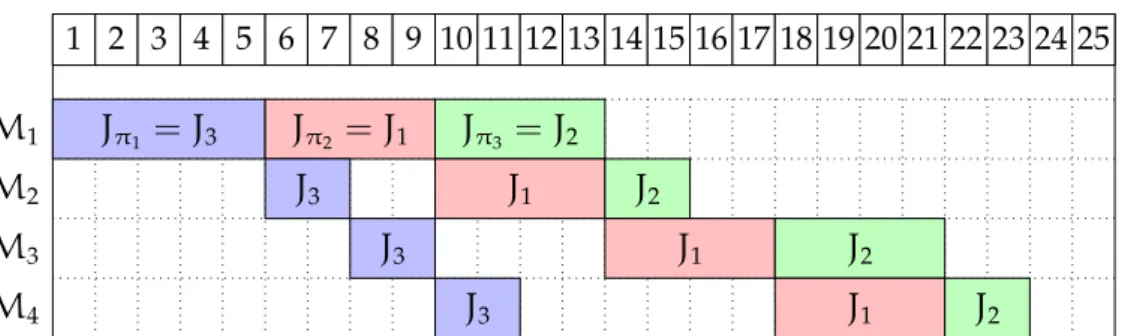
(34) Thèse de Aymeric Blot, Université de Lille, 2018. 18. Chapter 1. Multi-objective Metaheuristics. n jobs {J1 , . . . , Jn } that need to be scheduled on a set of m machines {M1 , . . . , Mm }. Each job Jk need to be processed sequentially on each of the m machines, with fixed processing times (pk,1 , . . . , pk,m ). Finally, machines are critical resources that can only process a single job at a time. For the permutation flow shop scheduling problem, each machine process the jobs in the same order, so that a solution may be represented by a permutation of size n. The completion times Ci,j for each job on each machine for a given permutation π = (π1 , . . . , πn ) are computed using Equation 1.8 to Equation 1.11. (1.8). Cπ1 ,1 := pπ1 ,1 Cπ1 ,j := Cπ1 ,j−1 + pπ1 ,j. ∀j ∈ {2, . . . , m}. (1.9). Cπi ,1 := Cπi−1 ,1 + pπi ,1. ∀i ∈ {2, . . . , n}. (1.10). Cπi ,j := max(Cπi−1 ,j , Cπi ,j−1 ) + pπi ,1. ∀i ∈ {2, . . . , n}. ∀j ∈ {2, . . . , m}. (1.11). The completion time Ck of a job Jk is then simply its completion time on the last machine Ck,m . An illustration of a small permutation flow shop instance (n = 3 jobs, m = 4 machines) is given in Figure 1.3. It features examples of waiting time, e.g., on machine M2 as job J1 is still being processed on machine M1 , and an example of idle time for job J2 on machine M3 as the processing of job J1 is not yet completed. The corresponding completions times of the three jobs J1 , J2 and J3 are 21, 23 and 11, respectively. 1 2 3 4 5 6 7 8 9 10 11 12 13 14 15 16 17 18 19 20 21 22 23 24 25. M1 M2 M3 M4. Jπ1 = J3. Jπ2 = J1. Jπ3 = J2. J3. J1 J3. J2 J1. J3. J2 J1. J2. Figure 1.3 – Example of PFSP schedule for n = 3 jobs, m = 4 machines, and π = (3, 1, 2) The most common objective to minimise on flow shop scheduling problem is the makespan (i.e., the total completion time of the schedule Cπn ,m , here 23 in Figure 1.3). Other classical objectives include the total flow time (i.e., the sum of completion times, and consequently their average), or when due dates are introduced, the maximum or total tardiness (Lawler et al., 1993). Weighted variants of these objectives are also common (Dubois-Lacoste et al., 2011b). In the following, we will study two bi-objective PFSP, with first a classical combination of. © 2018 Tous droits réservés.. lilliad.univ-lille.fr.

(35) Thèse de Aymeric Blot, Université de Lille, 2018. 1.3. Permutation Problems. 19. makespan and total flow time (Dubois-Lacoste et al., 2011c; Bezerra et al., 2014). Because the makespan and total flow time objective are quite correlated, we will also study a second bi-objective PFSP, obtained by considering a combination of two makespan objectives computed with hand-tuned correlated processing times (Kessaci-Marmion et al., 2017). The classical literature PFSP instances are given by Taillard (1993). They are randomly generated with independent processing times following the uniform distribution U[1; 99]. There are 110 Taillard’s instances, with number of jobs n ∈ {20, 50, 100, 200, 500} and number of machines m ∈ {5, 10, 20}, 10 instances being available for each valid combination (n, m). Classical PFSP neighbourhoods include the exchange neighbourhood, where the positions of two jobs are exchanged, and the insertion neighbourhood, where one job is reinserted at another position in the permutation. It was shown that for multi-objective local search algorithms the hybrid neighbourhood defined as the union of the exchange and insertion neighbourhoods lead to better performance than considering a single neighbourhood (Dubois-Lacoste et al., 2015). Other common operations on schedules include the adjacent swap, special case of exchange when the two jobs are necessary adjacent – thus highly reducing the computational cost but also the interest of such an operation – or the block-move, generalisation of both the insertion and the adjacent swap when the positions of two adjacent subsets of jobs are exchanged. Block-moves are less commonly used as they induce much bigger neighbourhoods. These operations are illustrated in Figure 1.4 starting from an ordered permutation. J1. J2. J6. J4. J5. J3. J7. J8. J1. (a) Exchange (J6 with J3 ). J1. J2. J3. J4. J6. J5. J7. J2. J6. J3. J4. J5. J7. J8. (b) Insertion (J6 before J3 ). J8. (c) Adjacent swap (J6 with J5 ). J1. J2. J6. J7. J3. J4. J5. J8. (d) Block-move ({J6 , J7 } with {J3 , J4 , J5 }). Figure 1.4 – Common PFSP schedule operations on an ordered permutation. 1.3.2. Travelling Salesman Problem. The travelling salesman problem (TSP) is one of the most widely studied combinatorial optimisation problems, optimising the tour of an hypothetical salesman. © 2018 Tous droits réservés.. lilliad.univ-lille.fr.

(36) Thèse de Aymeric Blot, Université de Lille, 2018. 20. Chapter 1. Multi-objective Metaheuristics. needing to visit once each of the n cities of a given set {C1 , C2 , . . . , Cn }. The TSP can be defined by a complete weighted graph G whose n nodes represent the cities, while edges corresponds to direct paths between cities. In the symmetric TSP, this graph is undirected, and edge weights correspond to distances between cities. Given a TSP instance G, the goal is to determine a tour passing through every city exactly once, such that the total distance travelled is minimised, i.e., a minimumweight Hamiltonian cycle in G. This cycle corresponds to a permutation of the n cities. There is no real meaning of the “beginning” or “direction” of the tour – e.g., for an instance with 4 cities the solutions (1, 2, 3, 4) and (2, 1, 4, 3) both map to the same tour – so permutations may need to be normalised (e.g., requiring to begin the tour with C1 and to visit C2 before C3 ) so that each possible tour has a unique representation. An illustration is given in Figure 1.5 for a small instance of n = 8 cities. C3. C4. C2. C5. C1. C6 C8. C7. Figure 1.5 – Example of TSP tour for n = 8 cities and π = (1, 2, 3, 8, 7, 5, 6, 4) Multi-objective TSP instances can easily be obtained by considering either correlated additional costs, such as distance and travel time, or simply multiple independent uncorrelated costs. A benchmark set of Euclidean instances (available online1 ) has been widely used in the literature to assess the performance of biobjective TSP algorithms. These instances were constructed by combining two independently generated distance matrices, the two objectives being therefore uncorrelated. In addition to these instances, we will also consider variably correlated instances, by first generating a set of cities, then duplicating it and slightly moving each city, to obtain two correlated matrices of Euclidean distances (KessaciMarmion et al., 2017). A classical neighbourhood for the travelling salesman problem is the 2-opt (or pairwise exchange) neighbourhood, where two tours are neighbours if, and only if, one can be obtained from the other by removing two non-adjacent edges reconnecting the resulting tour fragments by two other edges. It has the visual property 1. © 2018 Tous droits réservés.. https://eden.dei.uc.pt/~paquete/tsp/#Exp2. lilliad.univ-lille.fr.

(37) Thèse de Aymeric Blot, Université de Lille, 2018. 1.3. Permutation Problems. 21. of repairing routes that cross themselves. An illustration is given by Figure 1.6, in which edges (C1 , C4 ) and (C3 , C8 ) are removed and reinserted, reordering the tour of cities {C1 , C2 , C3 } to remove the crossing. Note that the 2-opt method is a special case of the more general k-opt method (or Lin–Kernighan method, Kernighan and Lin (1970); Lin and Kernighan (1973)), but that using k > 2 usually leads to a much bigger neighbourhood size and thus far higher computational cost. The permutation neighbourhoods (e.g., exchange, insertion; see Figure 1.4) can also be used on the TSP, albeit much less used and efficient than the k-opt methods. C3. C3. C4. C4. C2. C5. C2. C5. C1. C6. C1. C6. C8. C8. C7. C7. Figure 1.6 – Example of 2-opt recombination (left: removal; right: reinsertion). 1.3.3. Quadratic Assignment Problem. The quadratic assignment problem (QAP) involves assigning a set of n facilities {F1 , F2 , . . . , Fn } to a set of n given locations {L1 , L2 , . . . , Ln }, minimising a cost function that depends both on the distance between locations and the flow between the facilities assigned to these locations. A solution is a permutation π = (π1 , . . . , πn ), where each location Lk is associated to the facility Fπk . The objective is then to minimise the cost C associated to the solution, defined by Equation 1.12 for a given permutation π, with wi,j the flow between facilities Fi and Fj , and di,j the distance between locations Li and Lj . C :=. n ∑ n ∑. wi,j dπi ,πj. (1.12). i=1 j=1. Figure 1.7 shows two solutions of a small QAP instance (n = 8), in which for clarity most of the flow is supposed equal to 0 and is not represented (otherwise the graph would necessarily be complete). This figure highlights that the locations are fixed, the permutation only changing the mapping according to which facilities are associated to locations. Similarly to the TSP, multi-objective QAP instances can be obtained by considering either correlated additional costs or multiple independent uncorrelated. © 2018 Tous droits réservés.. lilliad.univ-lille.fr.

(38) Thèse de Aymeric Blot, Université de Lille, 2018. 22. Chapter 1. Multi-objective Metaheuristics L3 F3. F4 L4. L3 F3. F7 L4. L2 F2. F5 L5. L2 F2. F5 L5. L1 F1. F6 L6. L1 F1. F6 L6. L8 F8. F7 L7. L8 F8. F4 L7. Figure 1.7 – Examples of QAP pairings for n = 8 locations (thus facilities); left: π = (1, 2, 3, 4, 5, 6, 7, 8); right: π = (1, 2, 3, 7, 5, 6, 4, 8) costs. To our present knowledge, there are publicly available multi-objective QAP instance generators (Knowles and Corne, 2003) but no widely recognised multiobjective QAP benchmarks in the literature. To obtain bi-objective instances, we consider two correlated flow matrices, both tied to a single distance matrix. As for both previous problems, it enables for the correlation between the two objectives to be manually adjusted (Kessaci-Marmion et al., 2017). The neighbourhood commonly used on QAP is the exchange neighbourhood (see Figure 1.4). Indeed, while other neighbourhood such as insertions or k-opt operations can be used, they have here no real meaning as positions in the permutation are not related in any way to an ordering of the facilities, but solely their mapping to the different locations, which stay fixed.. © 2018 Tous droits réservés.. lilliad.univ-lille.fr.

(39) Thèse de Aymeric Blot, Université de Lille, 2018. Chapter 2 Automatic Algorithm Design If I have seen further it is by standing on the shoulders of Giants. Isaac Newton. In this chapter, we present the research field of automatic algorithm design (AAD). After some necessary preliminary definitions, we give an overview of the different research fields of the literature, such as automatic algorithm control, algorithm selection, hyper-heuristics, and state of the art methods that are related to AAD. Then, we propose and discuss a new taxonomy of AAD to better group under a single label these research fields.. In the process of solving problems and obtaining solutions, one generally needs to go through many analysis, decisional and computational steps, steps that may be automatised with the use of algorithms. The usual procedure is to: (i) formally define the problem to solve, (ii) either choose an existing algorithm or design a new specific one to solve the problem, (iii) run the algorithm on the particular input of interest, to finally (iv) obtain relevant solutions. These steps describe an algorithm, for the theoretical higher-order “problem solving” problem. More particularly, the second step is related to answering the question “which algorithm should I use to solve my problem”, which can also be better worded as “what is the best algorithm to solve this problem”. While these questions are generally left to human expertise, they can be tackled automatically, through what we call automatic algorithm design. 23. © 2018 Tous droits réservés.. lilliad.univ-lille.fr.

(40) Thèse de Aymeric Blot, Université de Lille, 2018. 24. Chapter 2. Automatic Algorithm Design. 2.1. Preliminaries. In order to better contextualise the automatic algorithm design research field and better compare the different algorithm design approaches, we first give the necessary definitions and notions regarding to algorithms and design choices. Problem: a description, semantic, and formal definition of the problem and the possible solutions (e.g., the travelling salesman problem (TSP)). (Problem) instance: the particular data, relative to a given problem, over which an algorithm is used to obtain final solutions (e.g., the graph of distances corresponding to a list of cities for the TSP). (Problem) instance class: a subset of problem instances sharing common characteristics (e.g., instances of the same size, sharing a similar structure, or originating from the same source). (Problem) instance feature: a measurable property or characteristic of the instance. Note that selection or extraction of instance features are in themselves very hard machine learning problems. Algorithm: a complete and unambiguous description of how to obtain solutions for a given problem instance; in the following, we also identify an algorithm to the decisional schedule it induces. Parameter: a decision point in an algorithm reflecting a design choice. Parameter value: the value associated to a given parameter. Parameterised algorithm: an algorithm exposing design choices as parameters; a set of default parameter values is usually available. (Algorithm) configuration: the set of parameter values necessary to run a parameterised algorithm, by specifying a setting to each of its parameters.. Virtually all algorithms are based on a succession of design choices that enables them to successfully run and achieve results. If some of these design choices may be left to the user discretion in the form of parameters, most of them are statically defined in the algorithm following early decisions of the algorithm designer. Each of these design choices ultimately heavily impact the performance of the algorithm. Nowadays the tendency is hopefully to propose frameworks more open in their design. Indeed, with more available parameters, they can potentially reach far better performance if adequately configured. Eventually, almost every design choice could potentially (and probably should) be automatically optimised (Hoos, 2012). Parameters are usually classified into three categories:. © 2018 Tous droits réservés.. lilliad.univ-lille.fr.

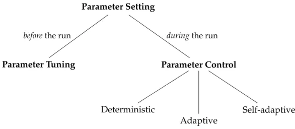
(41) Thèse de Aymeric Blot, Université de Lille, 2018. 2.2. Overview. 25. Categorical parameters, which have a finite number of unordered discrete values, often used to select between alternatives mechanisms (e.g., to select a specific strategy, or to enable or disable a mechanism); Integer parameters, which have discrete and ordered domains (e.g., to specify a number of iterations or the size of a set of solutions); and Continuous parameters, that take numerical values on a continuous scale (e.g., to set a probability or percentage threshold). The distinction between structural parameters (i.e., categorical parameters, or integer parameter with high impact on the comportment of the algorithm) and behavioural parameters (i.e., other integer and continuous parameters) is also common, under many different appellations: qualitative/quantitative, symbolic/numeric, categorical/numerical, component/parameter, nominal/ordinal, or categorical/ordered (see Eiben and Smit, 2012). In addition, some conditional parameters may only be used depending on the setting of other parameters, and some combinations of parameters may be forbidden when they are known to lead to incorrect or undesirable algorithmic behaviour.. 2.2. Overview. Offline approaches are usually opposed to online approaches (Hamadi et al., 2012), following the taxonomy of Eiben et al. (1999) of parameter setting (Figure 2.1), which divides parameter tuning approaches, which aim to find good values for the parameters before the run of the algorithm, and parameter control approaches, which start the run with initial parameter values that are then controlled and adapted during the run. Parameter Setting before the run. during the run. Parameter Tuning. Parameter Control. Deterministic. Self-adaptive Adaptive. Figure 2.1 – Eiben et al. (1999) parameter setting taxonomy. © 2018 Tous droits réservés.. lilliad.univ-lille.fr.

(42) Thèse de Aymeric Blot, Université de Lille, 2018. 26. Chapter 2. Automatic Algorithm Design. Offline approaches (parameter setting) focus on getting the best possible algorithm prior of its actual use on the input data; once the algorithm is fixed it runs following its specification. They can therefore be seen as prediction-based approaches. Conversely, online approaches (parameter control) do not predict the best possible algorithm but rather focus on optimising its configuration during its execution. In other words, online approaches try to adapt the schedule of decisional and computational steps of the algorithm using its impact on the input data, while offline approaches try to predict the entire fixed schedule. Of course, if this theoretically leads to much more efficient algorithms, general automatic adaption in algorithms is orders of magnitude more complex than just optimising over all possible static algorithms. This distinction between offline and online approaches deeply shaped the research on automatic algorithm design. Finally, to quote Karafotias et al. (2015) on the tuning and control of evolutionary algorithms: ‘From a practical perspective, tuning is an absolute ‘must’ [. . .] Meanwhile, parameter control is more of a neat-to-have than a need-to-have. ’ In the following, we present and discuss many of the research fields related to AAD, and how they differ between each others. While fields such as algorithm configuration and parameter control directly falls under Eiben taxonomy, we observe than many others such as algorithm selection or hyper-heuristics also closely relates to the same problematic: automatically devising better algorithms for given problems.. 2.2.1. Algorithm Selection. Algorithm selection focuses on understanding the relation between algorithm performance and problem instance features. The basis is that, for a given set of problem instance classes, there is a corresponding set of complementary algorithms that can be used to improve overall performance. Formally (Rice, 1976), the algorithm selection problem consists in, given a portfolio P of algorithms A ∈ P, a set of instances I, and a cost metric o : P × I → R, optimising a mapping s : I → P across all instances of i ∈ I, as given in Equation 2.1. ⎧ ∑ ⎨ optimise o(s(i), i) i∈I. ⎩ subject to s : I → P. (2.1). Because this problem optimises the performance on each instance of the set independently, algorithm selection is also sometimes called per-instance algorithm. © 2018 Tous droits réservés.. lilliad.univ-lille.fr.

(43) Thèse de Aymeric Blot, Université de Lille, 2018. 2.2. Overview. 27. selection. A simplified general workflow of algorithm selection is given in Figure 2.2., in which a selection tool construct the final mapping by iteratively providing an algorithm A and an instance i to a runner, whose role is to simply returns the subsequent performance. Portfolio P Instance set I. Mapping I → P. Selection tool. instance i ∈ I,. performance o(A, i). algorithm A ∈ P. Runner Figure 2.2 – Algorithm selection general workflow Some of the most prominent algorithm selection tools include SATzilla (Xu et al., 2008), ISAC (Kadioglu et al., 2010), 3S (Kadioglu et al., 2011) and CSHC (Malitsky et al., 2013). A recent extensive survey on algorithm selection for combinatorial search problem can by found in Kotthoff (2016), which also keeps an up to date online literature summary on algorithm selection literature1 . One extension of the traditional per-instance algorithm selection problem is perinstance algorithm scheduling, that associates to each instance not a single algorithm anymore, but a schedule of different algorithms. This extension allows to increase robustness, in particular regarding instances for which multiple algorithms might perform well. The algorithm schedules can be optimised globally for all instances (Hoos et al., 2015), determined for each instance relatively to algorithm performance on similar instances (Amadini et al., 2014), or used statically as a pre-solving mechanism before traditional algorithm selection (Kadioglu et al., 2010, 2011; Hoos et al., 2014). These approaches have been shown to be very efficient and to achieve strong performance on many algorithm selection scenarios (Lindauer et al., 2016).. 2.2.2. Algorithm Configuration / Parameter Tuning. Algorithm configuration (or parameter tuning) focuses on getting the best performance of a given algorithm on a given distribution of instances, through modifications of its parameters. The algorithm being optimised is called the target algorithm, while the algorithm optimising the parameters of the target algorithm is 1. https://larskotthoff.github.io/assurvey/. © 2018 Tous droits réservés.. lilliad.univ-lille.fr.