Pépite | Modélisation numérique des propriétés de coeurs de dislocations dans l’Olivine (Mg2SiO4)
118
0
0
Texte intégral
(2) Thèse de Srinivasan Mahendran, Université de Lille, 2018. © 2018 Tous droits réservés.. lilliad.univ-lille.fr.
(3) Thèse de Srinivasan Mahendran, Université de Lille, 2018. Thesis Presented at. l’Université de Lille Ecole doctorale Sciences de la Matière, du Rayonnement et de l’Environnement. To obtain the degree of. Docteur De l’Université In Materials Science. Srinivasan MAHENDRAN Numerical modelling of dislocation core properties in olivine (Mg2SiO4). Defence scheduled on 3 July 2018, before the jury composed of Prof. Sandrine BROCHARD. Dr. Andréa TOMMASI. University of Poitiers International Centre for Theoretical Physics, Trieste University of Montpellier 2. Examiner. Dr. Andrew WALKER. University of Leeds. Examiner. Prof. Philippe CARREZ. University of Lille. Supervisor. Prof. Patrick CORDIER. University of Lille. Co-supervisor. Prof. Sandro SCANDOLO. © 2018 Tous droits réservés.. Reviewer Reviewer. lilliad.univ-lille.fr.
(4) Thèse de Srinivasan Mahendran, Université de Lille, 2018. © 2018 Tous droits réservés.. lilliad.univ-lille.fr.
(5) Thèse de Srinivasan Mahendran, Université de Lille, 2018. Abstract Convection is a heat transfer process in which heat in the system is transmitted in a fluid like manner. It is widely accepted that the dissipation of heat from the core to the surface of the Earth through a thermally insulating mantle is only possible by a convective process. Mantle convection is responsible for a large number of geological activities that occur on the surface of the Earth such as plate tectonic, volcanism, etc. It involves plastic deformation of mantle minerals. Among the several layers of the Earth’s interior, the outer most layer beneath the thin crust is the upper mantle. One of the most common minerals found in the upper mantle is the olivine (Mg,Fe)2SiO4. Knowledge of the deformation mechanisms of olivine is important for the understanding of flow and seismic anisotropy in the Earth’s upper mantle. Plastic deformation of olivine has been the subject of numerous experimental studies highlighting the importance of dislocations of Burgers vector [100] and [001]. In this work, we report a numerical modelling at the atomic scale of dislocation core structures and slip system properties in Mg2SiO4 forsterite, at pressures relevant to upper mantle conditions. Computations are performed using the so-called THB1 empirical potential set for Mg2SiO4 and molecular statics. The energy landscape associated with the dislocation mobility are computed with the help of nudge elastic band calculations. Therefore, with this work, we were able to accurately predict the different possible dislocation core structures and some of their intrinsic properties. In particular, we show that at ambient pressure [100](010) and [001]{110} correspond to the primary slip systems of forsterite. Moreover, we propose an explanation for the so-called “pencil glide” mechanism based on the occurrence of several dislocation core configurations for the screw dislocation of [100] Burgers vector. Finally, the modelling of the intrinsic dislocation properties in a pressure range relevant of the Earth’s upper mantle allows to address the effect of high pressure on the primary slip systems of olivine.. © 2018 Tous droits réservés.. lilliad.univ-lille.fr.
(6) Thèse de Srinivasan Mahendran, Université de Lille, 2018. Résumé Il est aujourd’hui largement accepté que les mécanismes de convection mantellique dans le manteau supérieur sont reliés aux propriétés plastiques de l’olivine constituant principale du manteau supérieur. Ce minéral, un silicate de composition (Mg,Fe)2SiO4, se déforme essentiellement par glissement de dislocations de vecteurs de Burgers [100] et [001]. Dans le cadre de ce travail de thèse, nous avons donc choisi de modéliser les propriétés de ces dislocations ainsi que les systèmes de glissement potentiels de l’olivine à partir de calculs à l’échelle atomique. L’ensemble des calculs ont été effectués à l’aide du potentiel THB1. Une fois les structures de cœurs des défauts déterminées, les paysages énergétiques associés au glissement des dislocations ont été analysés par la méthode « Nudge Elastic Band ». A basse pression, la modélisation atomique montre que les systèmes [100](010) et [001]{110} correspondent aux systèmes de glissement primaires de l’olivine. L’étude des paysages énergétiques des dislocations nous permet de plus de rationaliser les observations expérimentales de « pencil glide » reportées dans l’olivine depuis les années 70 et de proposer un mécanisme original de blocage-déblocage pour le glissement des dislocations de vecteurs de Burgers [001]. Enfin, l’application de ce type de modélisation aux conditions de pression du manteau supérieur (0-10 GPa) confirme l’existence d’un effet de durcissement de la pression sur le glissement des dislocations de vecteur de Burgers [100].. © 2018 Tous droits réservés.. lilliad.univ-lille.fr.
(7) Thèse de Srinivasan Mahendran, Université de Lille, 2018. Table of contents 1. Introduction……………………………………………………………………11 1.1. Earth’s interior…………………………………………………………….11 1.2. Olivine crystal structure……………………………………………….......13 1.3. Elastic properties of olivine……………………………………………….15 1.4. Plastic properties of olivine……………………………………………….16 1.5. Plan of thesis………………………………………………………………20 2. Model and methodology……………………………………………………….23 2.1 Interatomic interactions…………………………………………………….23 2.1.1 Ionic polarisation……………………………………………………..25 2.1.2 The core-shell model…………………………………………………25 2.1.3 THB1 Potential library……………………………………………….27 2.2 Ground state properties…………………………………………………….31 2.2.1 Energy minimisation…………………………………………………31 2.2.2 Nudged elastic band approach……………………………………….32 2.3 Dislocations modelling…………………………………………………….34 2.4 Atomistic modelling………………………………………………………..37 2.4.1 Slab type system……………………………………………………...37 2.4.2 Quadrupole system……………………………………………….......38 2.5 Dislocation motion…………………………………………………………39 3. Implementation and validation of THB1 potential library………………….41 3.1 LAMMPS dependencies…………………………………………………...41 3.2 Force fields…………………………………………………………………42 7 © 2018 Tous droits réservés.. lilliad.univ-lille.fr.
(8) Thèse de Srinivasan Mahendran, Université de Lille, 2018. 3.3 Command description ……………………………………………………...44 3.4 Validation of THB1 potential………………………………………………46 3.4.1 Lattice constants……………………………………………………...46 3.4.2 Elastic constants……………………………………………………...48 3.4.3 Generalised stacking fault energy……………………………………51 3.5 Summary…………………………………………………………………...59 4. [100] Screw dislocations..……………………………………………………...61 4.1 Screw dislocation core at 0 GPa…………………………………………...61 4.1.1 Dislocation core structure……………………………………………61 4.1.2. Lattice friction……………………………………………………….64 4.2 Effect of pressure on dislocation core……………………………………...69 4.2.1 Low pressure core configuration……………………………………..69 4.2.2 High pressure core configurations…………………………………...74 4.3 Transition path from low pressure core to high pressure core configurations………………………………………78 4.4. Summary…………………………………………………………………..80 5. [001] screw dislocations..………………………………………………………83 5.1. Dislocation core structure at 0 GPa………………………………………..83 5.2. Core energy comparison at 0 GPa…………………………………………88 5.3. Lattice friction at 0 GPa…………………………………………………...89 5.4. Effect of pressure on [001] dislocation……………………………………92 5.5. Summary…………………………………………………………………..93 6. Discussion……………………………………………………………………….95. 8 © 2018 Tous droits réservés.. lilliad.univ-lille.fr.
(9) Thèse de Srinivasan Mahendran, Université de Lille, 2018. 6.1. Core configuration at 0 GPa……………………………………………….95 6.2. Locking-unlocking mechanism……………………………………………95 6.3. Effects of pressure…………………………………………………………97 6.4. Pencil glide for [100] dislocations………………………………………...98 6.5. Summary…………………………………………………………………..99 7. Conclusion……………………………………………………………………..101 Bibliography……………………………………………………………………...105 List of abbreviations……………………………………………………………..115 Acknowledgements………………………………………………………………117. 9 © 2018 Tous droits réservés.. lilliad.univ-lille.fr.
(10) Thèse de Srinivasan Mahendran, Université de Lille, 2018. 10 © 2018 Tous droits réservés.. lilliad.univ-lille.fr.
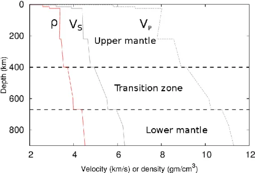
(11) Thèse de Srinivasan Mahendran, Université de Lille, 2018. Introduction. Chapter 1. 1. Introduction After 4.6 billion years since the formation of the Earth, its interior is still hot. The heat flux coming towards the Earth surface is measured to be about 46±3 TW for the whole planet (Jaupart and Mareschal 2015). How is this heat transferred to the surface? Since rocks are opaque and insulating, mantle convection is widely accepted to be the major contributor for the transfer of heat to the surface, and the Earth’s mantle can be considered to behave over geological timescales as a fluid endowed with a very high viscosity (1021-1022 Pa s) (Yokokura 1981). The convection movements occur by the plastic deformation of rocks, which is controlled by the plastic properties and chemical composition of their constituent minerals. Plastic deformation occurs through the deformation of the constituent crystals; this involves migration of defects such as point defects, dislocations, grain boundaries, etc. The knowledge on these defects helps us to link our understanding on the microscopic scale with the behaviours observed at macroscopic scale.. 1.1. Earth’s interior The mineral olivine forms a solid solution between forsterite (Mg2SiO4) and fayalite (Fe2SiO4). Being one of the most abundant mineral in the Earth’s upper mantle, olivine is a key mineral which controls the rheology of the upper mantle. The Earth’s interior is divided into several layers; the upper mantle corresponds to the first subdivision of it, as deduced from the analysis of the time travel of seismic waves. One of the standards among seismological models is the preliminary reference Earth model (PREM) proposed by Dziewonski and Anderson (1981) (Figure 1.1). This is one-dimensional model in which all the physical parameters are assumed to change with depth only. According to seismic information, several discontinuities are observed in the Earth’s interior. The crust is the upper most divided into oceanic and continental crust (~7 – 70 km), below is the mantle divided into two layers, the upper mantle (~410 km) and the lower mantle (~670 – 2890 km), with a transition zone (~410 – 670 km) sandwiched between the two mantle layers and the Earth core (~2890 – 6370 km) subdivided into a liquid outer core and a solid inner core.. 11 © 2018 Tous droits réservés.. lilliad.univ-lille.fr.
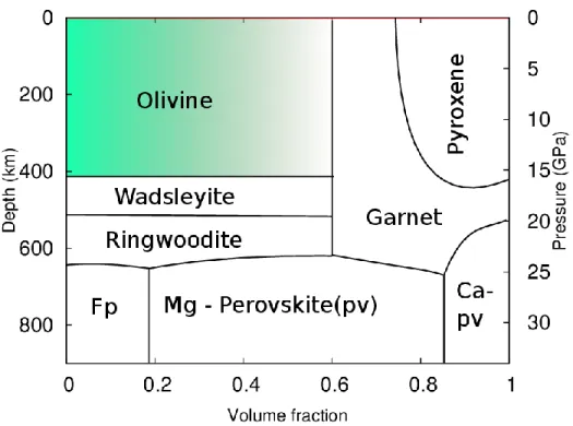
(12) Thèse de Srinivasan Mahendran, Université de Lille, 2018. Chapter 1. Introduction. Figure 1.1. Preliminary reference Earth model (PREM) from Dziewonski and Anderson (1981). Density and seismic velocities plotted as a function of depth.. The data available on seismic wave velocities are mostly influenced by the density and the elastic properties of the rock aggregates. For instance, the outer core is known to be made mainly of liquid, as the shear waves vanish and the compression waves are solely recorded. Therefore, the discontinuities in PREM model can be interpreted as transformation of rock aggregates or material. Such modifications being driven by thermodynamics stability of minerals as pressure and temperature increase with depth. Ringwood (1962; 1975) proposed a model on the chemical composition of the upper mantle known as the pyrolytic model. Based on this model (Figure 1.2), the upper mantle is composed of olivine (Mg,Fe)2SiO4, pyroxene (Mg,Fe,Ca)2Si2O6 and garnets (Mg,Fe,Ca)3Al2Si3O12. At ~410 km, the pressure and temperature in the mantle reaches 13 GPa and 1400 °C respectively, under these conditions olivine transforms into a highpressure polymorph named wadsleyite. Deeper into the transition zone (~520 km) wadsleyite transforms into ringwoodite, a denser high-pressure polymorph of olivine. At depths beyond ~670 km, (where the P, T conditions are 23 GPa, 1600 °C), ringwoodite and garnets decompose into a two-phases aggregate composed of a silicate with a perovskite structure now known as bridgmanite and ferropericlase (Fp) (Mg,Fe)O. 12 © 2018 Tous droits réservés.. lilliad.univ-lille.fr.
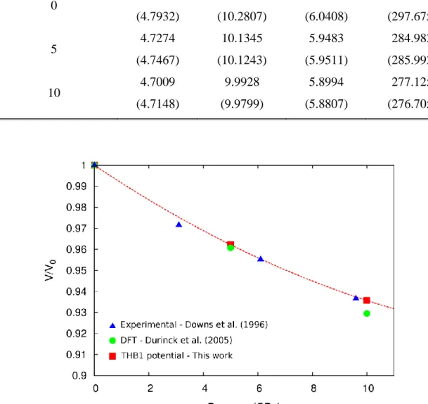
(13) Thèse de Srinivasan Mahendran, Université de Lille, 2018. Introduction. Chapter 1. Figure 1.2. Simplified mineralogy of the pyrolytic mantle layers of the Earth as a function of depth, pressure and volume fraction (Brown and Shankland (1981)).. 1.2. Olivine crystal structure Olivine is an olive green mineral which exists as a solid solution of (Mg,Fe)2SiO4. In this thesis, we will focus on the magnesium-rich end-member forsterite (Mg2SiO4). It is close to the average composition of olivine in the upper mantle which contains a little bit less than 10% of iron. The melting point of forsterite and fayalite are 2163 K and 1473 K respectively (Bowen and Andersen 1914; Ohtani and Kumazawa 1981; Klein and Hurlbut 1999). Forsterite corresponds to an orthorhombic crystal structure, which can be described within the Pbnm space group. The crystal structure which contains isolated SiO4 tetrahedra can be viewed as slightly distorted hexagonal close packed (hcp) lattice of oxygen anions (Poirier 1975), with one eighth of the octahedral sites occupied by magnesium cations. In the Pbnm space group, the lattice constants (at ambient pressure and temperature) are a = 4.756 Å, b = 10.207 Å, c = 5.98 Å (Smyth and Hazen 1973).. 13 © 2018 Tous droits réservés.. lilliad.univ-lille.fr.
(14) Thèse de Srinivasan Mahendran, Université de Lille, 2018. Chapter 1. Introduction. Figure 1.3. The structure of orthorhombic forsterite, the Mg rich end-member of olivine described here with the Pbnm space group. The crystal structure projected along (a) [100] (b) [010] (c) [001] directions with unit cell marked with black line. Magnesium atoms are in yellow, oxygen is in red and silicon is in blue, located inside the SiO4 tetrahedral units. The isolated SiO4 tetrahedra are joined by Mg cations located in the M1 sites at the inversion centres. The Mg cations in the M2 site lie on a mirror plane.. Figure 1.3 (a) shows the projection of forsterite unit cell SiO4 tetrahedra viewed along [100] direction. The isolated tetraheadra point alternatively up and down along rows parallel to [001]. Each level of isolated tetrahedra are connected via octahedra containing 14 © 2018 Tous droits réservés.. lilliad.univ-lille.fr.
(15) Thèse de Srinivasan Mahendran, Université de Lille, 2018. Introduction. Chapter 1. metallic cations (Mg2+). The metal cations M1 lie in the inversion centres between two SiO4 tetrahedral units and M2 cations lie in the mirror plane (Deer et al. 1982).. 1.3. Elastic properties of olivine Based on the orthorhombic crystal symmetry, the elastic stiffness matrix, 𝐶𝑖𝑗 , of olivine consists of nine independent elastic constants.. C11 C12 C 21 C 22 C 31 C 32 0 0 0 0 0 0. C13 C 23 C 33 0 0 0. 0 0 0 C 44 0 0. 0 0 0 0 C 55 0. 0 0 0 0 0 C 66 . The nine elastic constant were initially determined by Isaak et al. (1989) at high temperature conditions. The effect of pressure on the elastic constants has been measured by Shimizu et al. (1982) and Zha et al. (1988) in a pressure range of 4 GPa and 16 GPa respectively (Table 1.1). The bulk modulus increases from 120 - 200 GPa and the shear modulus increases from 80 - 90 GPa at a pressure range of 0 – 16 GPa (Li et al. 1996; Zha et al. 1996; Yoneda and Morioka 1992) (Figure 1.4).. Table 1.1. Single crystal elastic moduli of San Carlos Olivine (in GPa) as a function of pressure. The experimental results are gathered from Zha et al. (1996). Pressure. 𝐶11. 𝐶22. 𝐶33. 𝐶44. 𝐶55. 𝐶66. 𝐶12. 𝐶13. 𝐶23. 2.5. 332.5. 209.4. 251.4. 68.7. 80.1. 82.7. 80.7. 80.2. 84.4. 5.0. 352.8. 224.2. 267.1. 70.8. 85.7. 90.2. 91.2. 92.7. 95.2. 8.1. 378.9. 244.0. 283.5. 77.6. 91.9. 96.3. 100.8. 102.3. 104.7. 14.1. 395.3. 270.4. 295.3. 81.2. 96.6. 103.6. 122.5. 118.0. 123.0. 18.8. 424.1. 270.4. 326.8. 86.3. 99.8. 112.8. 129.2. 133.2. 138.2. (GPa). 15 © 2018 Tous droits réservés.. lilliad.univ-lille.fr.
(16) Thèse de Srinivasan Mahendran, Université de Lille, 2018. Chapter 1. Introduction. Figure 1.4. Evolution of Bulk (K) and shear modulus (µ) as a function of pressure experimentally determined for single crystal San Carlos olivine (Zha et al. 1996). The data yields a pressure derivative of 𝐾0′ = 4 and µ′0 = 1.6 the values compares well with values of 𝐾0′ = 4.4 and µ′0 = 1.3 (Li et al. 1996).. 1.4. Plastic properties of olivine For modelling the convection of the Earth’s mantle, one needs information on the plastic properties of the constitutive materials, starting with olivine. As the elastic energy of a dislocation is proportional to the square of Burgers vector (𝐸𝑒𝑙 ∝ 𝑏2), this relation makes [010] dislocation energetically least favourable. Based on the hexagonal close packed arrangement of oxygen sub-lattice, Poirier (1975) further proposed the following slip systems: [001] dislocation gliding in (100), (010), {110} and [100] dislocation gliding in (010), (001), {011} and {031} (Figure 1.5).. 16 © 2018 Tous droits réservés.. lilliad.univ-lille.fr.
(17) Thèse de Srinivasan Mahendran, Université de Lille, 2018. Introduction. Chapter 1. Figure 1.5. Forsterite unit cell with possible slip planes of (a) [100] and (b) [001] dislocations.. In natural samples, from the observations made with optical microscopy and transmission electron microscopy (TEM) techniques, one confirms that glide along [010] is unfavourable. Only dislocations with [100] and [001] Burgers vectors are commonly observed, whereas precise determination of slip systems is difficult and almost all the potential glides plane have been reported (Gueguen 1979; Kohlstedt et al. 1976). From the deformation experiment performed at ambient pressure on polycrystalline olivine Raleigh (1968) shows that the plastic deformation results from activation of [001] dislocations at low temperature and high stress condition, whereas at temperature above 1000 °C Carter and Ave’Lallemant (1970) observed activation of [100] dislocations. At temperature greater than 1300 °C, only [100](010) seems to be activated. To proceed further, deformation experiments have been performed on single crystals. Based on the 17 © 2018 Tous droits réservés.. lilliad.univ-lille.fr.
(18) Thèse de Srinivasan Mahendran, Université de Lille, 2018. Chapter 1. Introduction. orientation of the single crystals, the activation of preferential slip planes can be analysed. From the experimental results (Phakey et al. 1972, Durham et al. 1977, Evans and Goetze 1979, Darot and Gueguen 1981, Gaboriaud et al. 1981, Gueguen and Darot 1982, Wang et al. 1988, Barber et al. 2010) [100] glide at high temperature and [001] glide at low temperature in various slip planes are observed. A composite non-crystallographic glide of [100] dislocation in {0kl} has long been reported (Raleigh 1968), such a mechanism is called the pencil glide.. Figure 1.6. Summary of critical resolved shear stress values for [100] dislocation glide, obtained from various single crystal deformation experiments. (adapted from the PhD thesis of Durinck (2005c)).. More importantly, deformation experiments performed on single crystals give access to quantitative information on the mechanical behaviour of slip systems. In particular, critical resolved shear stress have been reported for at least four slip systems: [100](010), [001](010), [001](100),[001]{110}. From Figure 1.7 it is visible that data are available for [001] glide at low temperature, unlike the case of [100] where the glide is observed only at high temperature experimental conditions Figure 1.6.. 18 © 2018 Tous droits réservés.. lilliad.univ-lille.fr.
(19) Thèse de Srinivasan Mahendran, Université de Lille, 2018. Introduction. Chapter 1. Figure 1.7. Summary of critical resolved shear stress values for [001] dislocation glide, obtained from various single crystal deformation experiments. (adapted from the PhD thesis of Durinck (2005c)).. In the context of upper mantle, temperature is not the only factor that influences the plastic properties. At depth close to the transition zone, the pressure in the mantle rises to 13 GPa. Also incorporation of water in the mantle is reported to influence plasticity. Thus, over the past two decades, deformation experiments have been performed to study the influence on plasticity due to the effect of pressure and the effect of incorporation of water. The experiments were carried out using both polycrystals and single crystals. For experiments performed with polycrystals, the analysis in terms of slip system is often performed through the analysis of crystal preferred orientation (CPO). According to change in CPO, Jung and Karato (2001) show that water has an influence on the preferential slip systems in olivine by promoting dislocation with [001] Burgers vectors. On the other hand, Couvy et al. (2004) show that pressure also strongly enhances activation of [100] glide under Earth mantle conditions (11 GPa, 1400 °C). Using single crystal deformation experiments, Raterron et al. (2005, 2007, 2009, 2011) reaches, with a series of single crystals deformation experiments at mantle pressure conditions a similar kind of conclusion, with an inversion of preferential slip system from [001] to [100] at high pressure. Several explanations have been proposed to support one or the other conclusion, however a full theoretical understanding is still needed. For instance, either pressure or water has an 19 © 2018 Tous droits réservés.. lilliad.univ-lille.fr.
(20) Thèse de Srinivasan Mahendran, Université de Lille, 2018. Chapter 1. Introduction. effect on dislocation activity, such effect may have its origin from the core structure of the defect. It is well known that fundamental properties of dislocations, such as lattice friction, glide velocity, and also in a lesser extent climb velocity, are directly related to the atomic arrangements within the vicinity of the dislocation core, or to impurities. Up to now, only a few works have been dedicated to study the atomic arrangement in the dislocation cores in olivine. The primary studies performed by Durinck and co-workers (2005a; 2005b; 2007) using Density Function Theory (DFT) calculations to compute generalised stacking fault (GSF) energies and to deduce the dislocation core configurations according to the Peierls Nabarro (PN) model. At the same period, Walker and co-workers (Walker et al. 2005a; Walker et al. 2005b; Carrez et al. 2008), used empirical potential models to compute dislocation core structures via atomistic simulations. However, due to the limitations in computational efficiency of the code existing at that time, mechanical properties have not been infered from the atomic core structure. The PN model is rather promising as it can provide some mechanical information through the computation of the Peierls stress, but has to be handled with great care while dealing with complex crystal structure. In general, the PN model gives satisfactory results in case of planar core configurations, it can also lead to several artefacts when the dislocations are non-planar or dissociated and computationally demanding (Schoeck 2005; 2006). 1.5. Plan of thesis In this work, we intent to revisit the dislocation core structures of olivine (Mg2SiO4). We investigate the two Burgers vector [100] and [001], over a pressure range 0-10 GPa corresponding to upper mantle conditions. This work only focuses on screw dislocations, since uncertainties remain on the slip systems. It is common to analysis the screw core configurations to infer the potential slip systems for the plane where the cores tend to spread. To avoid artefacts encountered in the past, approaches such as PN model or generalisation of PN model will not be used, and we will perform full atomistic calculations. But still Peierls stresses determination will be carried out directly from the atomic configuration. Also as an advantage, full atomistic calculations give access to the energetic landscape around dislocation core. As described in the following chapter, the energy landscape along dislocation pathway will be computed using nudged elastic band (NEB) approach, a method used to investigate transition state paths. The results presented 20 © 2018 Tous droits réservés.. lilliad.univ-lille.fr.
(21) Thèse de Srinivasan Mahendran, Université de Lille, 2018. Introduction. Chapter 1. in chapters 4 and 5 correspond to [100] and [001] dislocation cores respectively. Finally, a discussion chapter will summarize our results and put them in perspective with the current state of the art of olivine plastic properties. As described in the following pages, we have chosen to work with the open-source classical molecular mechanics code called the LAMMPS and the THB1 force field to describe forsterite. At the beginning of this work, THB1 potential was not available into LAMMPS, chapter 3 is thus a technical chapter dedicated to our implementation of THB1 potential model to LAMMPS library and some important checkpoints computations performed before addressing the heart of this thesis.. 21 © 2018 Tous droits réservés.. lilliad.univ-lille.fr.
(22) Thèse de Srinivasan Mahendran, Université de Lille, 2018. Chapter 1. Introduction. 22 © 2018 Tous droits réservés.. lilliad.univ-lille.fr.
(23) Thèse de Srinivasan Mahendran, Université de Lille, 2018. Model and methodology. Chapter 2. 2. Model and methodology Interatomic pair potentials play a significant role in performing molecular and materials simulation. In the process of modelling ionic or semi-ionic material like forsterite, various key parameters have to be considered. This chapter introduces basics of pairwise potential model; followed by the necessity of an interatomic potential library with core-shell approximation. The potential energy and its corresponding force fields are the basic input for the energy minimization and transition path algorithms. This chapter further introduces basic methodology of atomistic simulations that are performed in this work to the study the dislocation core structure and mobility of dislocation.. 2.1 Interatomic interactions Quantum mechanical methods can be used to predict mechanical behaviour and properties of materials accurately but are computationally expensive to model systems of large dimensions (i.e., having few thousand atoms). The task of modelling dislocations and defects in olivine involves systems too large to be solved quantum mechanically. The density function theory (DFT) provides amendable numerical solutions to Schrodinger’s equation. It is accepted as a strong method to solve bonding problems, whereas the expense of computational cost limits the simulation to few hundreds of atoms. Alternatively, tight-binding (TB) methods. reduces the computational cost by. parameterising many DFT integrals, whereas its description of electronic structure consisting of neutral atoms makes it difficult to model ionic systems. Force fields methods ignore the electron field and calculates energy (U) as an analytical/numerical function based on nuclear positions (equation 2.1). 𝑈 = 𝑈(𝑟1 , 𝑟2 , 𝑟3 … 𝑟𝑁 ). (2.1). 𝑁. 𝑁. 𝑁. 𝑁. 𝑁. 𝑁. 𝑖. 𝑖. 𝑗. 𝑖. 𝑗. 𝑘. 1 1 𝑈 = ∑ 𝑈𝑖 + ∑ ∑ 𝑈𝑖𝑗 + ∑ ∑ ∑ 𝑈𝑖𝑗𝑘 + ⋯ 2! 3!. (2.2). Here, the total energy of the system can be decomposed into interactions between different numbers of atoms or ions as in equation 2.2. 𝑈𝑖 represents the self-energy of the atoms. 𝑈𝑖𝑗 is the pairwise potential energy term that can be written as a sum of interaction of two 23 © 2018 Tous droits réservés.. lilliad.univ-lille.fr.
(24) Thèse de Srinivasan Mahendran, Université de Lille, 2018. Chapter 2. Model and methodology. atoms i and j separated by a distance 𝑟𝑖𝑗 . When a triad of atoms is considered, their energy of interaction is given by 𝑈𝑖𝑗𝑘 . For example, the Stillinger-Weber potential (Stillinger and Weber 1985) used for a system of silicon atoms, includes two-body and three-body interactions. The three-body term penalizes the deviation of bond angle from tetrahedral angle (109.47 degree). The above decomposition is more accurate when order of interaction increases, but it is important to truncate the order at some stage. This superposition of pairwise interactions works well to model ionic materials and semiconductor materials, as the bonds are well localised. Unlike for the case of metals the bonds are shared by many atoms. The embedded atom method (EAM) (Daw and Baskes 1984) is a well-suited model for atomistic modelling of metals. The embedded function of the EAM function is non-linear, and the many-body term included in this approach cannot be reproduced by superposition of any order of pairwise interactions. In the following, we describe more precisely the modelling of ionic systems. Initially for modelling ionic or semi-ionic materials, only two body terms are considered. For a simple case, one can imagine an ionic solid being made of cations and anions, with frozen electron densities. In such cases the opposite charged ions attract each other due to Coulombic attraction and the like charged ions experience a similar repulsive force. The closest neighbour ions with opposite charges result in a strong net attractive force, which will tend to contract the system to arrive in a lower energy configuration. In order to bring the system in equilibrium a counter balancing repulsive force is required. This force can be obtained from the overlap of electron density of two ions, irrespective of the type of charge, which can be explained by Pauli repulsion between electrons. Thus the total energy of the system can be expressed as follows: 𝑈𝑇𝑜𝑡𝑎𝑙 = 𝑈𝐶𝑜𝑢𝑙𝑜𝑚𝑏 + 𝑈𝑆ℎ𝑜𝑟𝑡. (2.3). Here in equation 2.3, the Coulomb energy, 𝑈𝐶𝑜𝑢𝑙𝑜𝑚𝑏 , is obtained by the summation of interactions of all atomic charges in the system, and this is an important component of cohesive energy. The short range energy term, 𝑈𝑆ℎ𝑜𝑟𝑡 , represents the rest of interactions in the system including Pauli repulsion, covalent and dispersive attractive terms.. 24 © 2018 Tous droits réservés.. lilliad.univ-lille.fr.
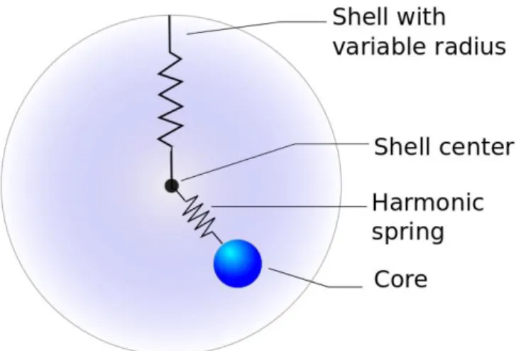
(25) Thèse de Srinivasan Mahendran, Université de Lille, 2018. Model and methodology. Chapter 2. 2.1.1 Ionic polarisation From the above explanation, the ions have a frozen spherical electron density and are represented with a point charge. This gives a simple representation, whereas for better accuracy it is necessary to include the effect of polarisation. For instance, in the case of an oxide with anion O2-, first electron affinity of oxygen is favourable, while the second electron affinity is endothermic due to the Coulombic repulsion term which is strongly perturbed by the local environment (Gale 2005). Hence it is necessary to include a polarisation term to produce reliable results. An additional point dipole term can be added to the point charge representation of ion. With inclusion of dipole polarisability 𝛼𝑃𝑜𝑙𝑎𝑟𝑖𝑠𝑎𝑡𝑖𝑜𝑛 , in presence of an electric field E the dipole moment µ is given in equation 2.4 which results in polarisation energy UPC (equation 2.5), results in a total energy combination given in equation 2.6. µ = 𝛼𝑃𝑜𝑙𝑎𝑟𝑖𝑠𝑎𝑡𝑖𝑜𝑛 𝐸. (2.4). 1 𝑈𝑃𝐶 = − 𝛼𝑃𝑜𝑙𝑎𝑟𝑖𝑠𝑎𝑡𝑖𝑜𝑛 𝐸 2 2. (2.5). 𝑈𝑇𝑜𝑡𝑎𝑙 = 𝑈𝐶𝑜𝑢𝑙𝑜𝑚𝑏 + 𝑈𝑆ℎ𝑜𝑟𝑡 + 𝑈𝑃𝐶. (2.6). Hence it is straightforward to include this polarisation self-energy contribution of each ion to the total energy. Whereas assuming a constant value of 𝛼𝑃𝑜𝑙𝑎𝑟𝑖𝑠𝑎𝑡𝑖𝑜𝑛 prevents the system to polarise further beyond this value. It leads to imbalance in the ratio of increase in attractive term compared to the repulsive term, results in collision of ions during defect calculations. When the distance between two ions is zero the short range term (1/r) tends to infinity numerically. To avoid this adverse effect, the value of polarisation has to be iteratively solved.. 2.1.2 The core-shell model The above discussed collision of ions may lead to polarisation catastrophe (Catlow et al. 1982; Gale 2005). This problem can be overcome by using the core-shell model, a mechanical description of ions proposed by Dick and Overhauser (1958). This model describes each ion as two particles, a massive “core” which represents the nucleus and core electrons, and a massless “shell” which represents the polarisable valance shell electrons. The core and shell are connected using a spring with a spring constant K. The core is 25 © 2018 Tous droits réservés.. lilliad.univ-lille.fr.
(26) Thèse de Srinivasan Mahendran, Université de Lille, 2018. Chapter 2. Model and methodology. positively charged and the shell is negatively charged. The sum of the charges gives the charge of the ion. Both core and shell holding a positive charge is common in representation of a cation. A schematic description of the core-shell model is given in figure 2.1. The dipole moment can be modelled by the displacement of shell with respect to the core. In such a description the 𝛼𝑃𝑜𝑙𝑎𝑟𝑖𝑠𝑎𝑡𝑖𝑜𝑛 can be related to the core-shell model parameters K and to the charge of the shell 𝑞𝑠ℎ𝑒𝑙𝑙 using a simple relation as follows: 𝛼𝑃𝑜𝑙𝑎𝑟𝑖𝑠𝑎𝑡𝑖𝑜𝑛 =. 2 𝑞𝑠ℎ𝑒𝑙𝑙 𝐾. (2.7). From this description the potential library will consists of a set of atoms with charges, analytical function to model Pauli’s repulsion and covalent terms and a representation of polarisation with core-shell model (Ucore-shell). Hence the split of energy is given as follows: 𝑈𝑇𝑜𝑡𝑎𝑙 = 𝑈𝐶𝑜𝑢𝑙𝑜𝑚𝑏 + 𝑈𝑆ℎ𝑜𝑟𝑡 + 𝑈𝑐𝑜𝑟𝑒−𝑠ℎ𝑒𝑙𝑙. (2.8). In this work, we use the core-shell model potential library THB1 proposed by Price and Parker (1987) to model forsterite and its high-pressure polymorphs. This library supplements an additional three-body term, which helps to include the covalence of the bonding within the SiO4 tetrahedra.. Figure 2.1. Schematic representation of an ion in the core-shell model. Each ion is made of two parts. The core represents the nucleus and the shell represents the electron cloud. These two parts are connected with each other using a harmonic spring.. 26 © 2018 Tous droits réservés.. lilliad.univ-lille.fr.
(27) Thèse de Srinivasan Mahendran, Université de Lille, 2018. Model and methodology. Chapter 2. The above mentioned core-shell approximation gives an effective solution to model ionic materials. However, the accuracy of core-shell methods suffers a drawback in computation of elastic constants and phonon dispersion curves in rock salts (like MgO, CaO, NaCl). In principle for centrosymmetric cubic crystals, the pairwise potential models obey Cauchy’s relation C44 = C12. But experimental results in rock salts suggests that C44/C12 > 1 (Matsui 1998). In order to solve this problem, the “breathing shell” model (Schroder 1966; Sangster et al. 1970; Sangster 1973) is found to be more accurate than the normal shell model in modelling of rock salts (Sangster et al. 1970, Matsui 1998). In this work for the modelling of forsterite silicate we keep a normal core-shell model library with THB1 parameterisation.. Figure 2.2. Schematic representation of an ion using breathing shell model. The shell has a variable radius, which is allowed to deform isotropically due to the effect of neighbouring ions. The core and the shell are connected using a harmonic spring.. 2.1.3 THB1 Potential library The THB1 potential is fully ionic empirical potential for accurate modelling the properties of forsterite (Mg2SiO4) and its high-pressure polymorphs. The effort of modelling forsterite using atomic simulation has a long and continuous history (Price and Parker 1984; Price et al. 1985 and Catlow et al. 1986). These models concentrated on the pairwise interactions but ignored the effect of many-body interactions. Whereas, the success of three-body interaction in modelling complex silicates (Matsui and Bushing 1984; Sanders 27 © 2018 Tous droits réservés.. lilliad.univ-lille.fr.
(28) Thèse de Srinivasan Mahendran, Université de Lille, 2018. Chapter 2. Model and methodology. et al. 1984) using bond-bending term, lead to the development of potential model of THB1 (Price and Parker 1987). The core-shell approximation enables every ion to polarize in response to an electric field due to the surrounding ions. Energy decomposition of THB1 model can be described as a summation of four terms as follows, 𝑈𝑇𝑜𝑡𝑎𝑙 = 𝑈𝐶𝑜𝑢𝑙𝑜𝑚𝑏 + 𝑈𝑆ℎ𝑜𝑟𝑡 + 𝑈𝑐𝑜𝑟𝑒−𝑠ℎ𝑒𝑙𝑙 + 𝑈𝑇𝐻𝐵. (2.9). 𝑈𝐶𝑜𝑢𝑙𝑜𝑚𝑏 represents the long range electrostatic energy term, which arrives as a result of summation of charges of atomic species present in the system. It is given by energy of electron e, point charges 𝑞𝑖 and 𝑞𝑗 associated with ions i and j respectively and the distance of separation between them. 𝑈𝐶𝑜𝑢𝑙𝑜𝑚𝑏 = ∑ 𝑒 2 𝑞𝑖 𝑞𝑗 𝑟𝑖𝑗−1. (2.10). 𝑖𝑗. The ionic materials pose additional challenge in computing the electrostatic term. Coulombic summation is a computationally expensive task due to the long-range character of the interaction. Traditionally the Coulomb summation results in converging of equations under specific conditions, particularly the Madelung problem (Madelung 1919; Gdoutos et al. 2010). The Madelung problem was solved with the Ewald summation (Ewald 1921), which through certain mathematical manipulations calculates the conditionally convergent 𝑂(𝑟 −1 ) Coulomb summation. The Ewald method assumes periodicity of the material. The result of this summation method is less reliable with non-periodic or quasi-periodic systems. Further, this method is computational expensive for large systems. To overcome these drawbacks, we replace the Coulomb term with a Wolf summation method (Wolf et al. 1999). The Wolf summation method for accumulation of electrostatic charges, involves a simple modification to the direct pairwise sum but scales approximately linearly with the system size (Fennel et al. 2006). 𝑈𝐶𝑜𝑢𝑙𝑜𝑚𝑏 = 𝑈𝑠ℎ − 𝑈𝑠𝑒𝑙𝑓. (2.11). 𝑁. 𝑈𝑠ℎ. 𝑞𝑖 𝑞𝑗 𝑒𝑟𝑓𝑐(𝛼𝑟𝑖𝑗 ) 𝑞𝑖 𝑞𝑗 𝑒𝑟𝑓𝑐(𝛼𝑟𝑖𝑗 ) 1 ≈ ∑ ∑ ( − lim { }) 𝑟𝑖𝑗 →𝑅𝑐 2 𝑟𝑖𝑗 𝑟𝑖𝑗 𝑖=1. 𝑗≠𝑖 (𝑟𝑖𝑗 <𝑅𝑐 ). (2.12). 𝑁. 𝑈𝑠𝑒𝑙𝑓. 𝑒𝑟𝑓𝑐(𝛼𝑅𝑐 ) 𝛼 2 =( + 1/2 ) ∑ 𝑞𝑖𝑜𝑛 𝑖 2𝑅𝑐 𝜋. (2.13). 𝑖=1. 28 © 2018 Tous droits réservés.. lilliad.univ-lille.fr.
(29) Thèse de Srinivasan Mahendran, Université de Lille, 2018. Model and methodology. Chapter 2. where α is the damping factor and 𝑅𝑐 is the cut-off distance for Columbic term. The Coulomb term is split into a charge neutralized Ewald potential term 𝑈𝑠ℎ and a self-energy term for each ion 𝑈𝑠𝑒𝑙𝑓 .. Figure 2.3. Schematic representation of interactions in the THB1 potential model.. Each ion is constituted of a nucleus and an electron cloud. 𝑈𝑆ℎ𝑜𝑟𝑡 is the short-ranged Buckingham potential term used to describe the effect of an electron cloud on nearest neighbour ions. This term is parametrized by three constants 𝐴𝑖𝑗 , 𝐵𝑖𝑗 and 𝐶𝑖𝑗 between ions i and j. 𝑈𝑆ℎ𝑜𝑟𝑡 = ∑ 𝐴𝑖𝑗 𝑒𝑥𝑝 (− 𝑖𝑗. 𝑟𝑖𝑗 ) − 𝐶𝑖𝑗 𝑟𝑖𝑗−6 𝐵𝑖𝑗. (2.14). In case of an ion, core and its shell are Coulombically screened from each other and only allowed to interact via the harmonic spring term 𝑈𝑐𝑜𝑟𝑒−𝑠ℎ𝑒𝑙𝑙 . Coupling between the core and its shell is described by this term, which requires shell spring constants 𝐾1𝑖 , 𝐾2𝑖 and the distance of separation between core and its corresponding shell 𝑟𝑖 , 𝑈𝑐𝑜𝑟𝑒−𝑠ℎ𝑒𝑙𝑙 =. 𝐾1𝑖 𝑟𝑖2 𝐾2𝑖 𝑟𝑖4 + 2 24. (2.15). 29 © 2018 Tous droits réservés.. lilliad.univ-lille.fr.
(30) Thèse de Srinivasan Mahendran, Université de Lille, 2018. Chapter 2. Model and methodology. Table 2.1. Parameters for the THB1 potential library proposed by Price and Parker (1987) to model forsterite. Charges (units of electronic charge). Core - shell spring constant (eV·Å-2). Ions. Cores. Shells. Mg. 2.0. Si. 4.0. O. 0.848190. -2.848190. A (eV). B (Å). C (eV·Å6). Si – O. 1283.90734. 0.32052. 10.66158. O–O. 22764.0. 0.149. 27.88. Mg – O. 1428.5. 0.29453. 0.0. 74.92038. Short range term. Harmonic three body term. O – Si - O. k (eV·rad-2). θ0 (degrees). 2.09724. 109.47. For accurate modelling of structure and properties of silicates, it is important to describe the directionality of Si-O bonding using a bond-bending term into the potential (Price and Parker 1987, Sanders et al 1984). For that purpose, THB1 uses a harmonic three-body 𝐵 term, with 𝑘𝑖𝑗𝑘 being a derivable spring constant, 𝜃𝑖𝑗𝑘 is the angle between the O-Si-O. three-body term and 𝜃0 is the constant tetrahedral angle (109.47). 𝐵 𝑈𝑇𝐻𝐵 = ∑ 𝑘𝑖𝑗𝑘 (𝜃𝑖𝑗𝑘 − 𝜃0 ). 2. (2.16). 𝑖𝑗𝑘. We implemented the described inter-atomic potential library and the corresponding force fields to LAMMPS molecular mechanics code. A schematic representation of allowed 30 © 2018 Tous droits réservés.. lilliad.univ-lille.fr.
(31) Thèse de Srinivasan Mahendran, Université de Lille, 2018. Model and methodology. Chapter 2. interactions between ions are given in Figure 2.3. The THB1 parameterization used in this work (Table 2.1) was previously derived by Price and Parker (1987) for forsterite.. 2.2 Ground state properties Using DFT or pairwise potential library like THB1 we can compute the potential energy of a system. In either methods, for a system containing N atoms with atomic positions ri = (r1, … rN) known, the potential energy can be computed at a given position, 𝑈 = 𝑈(𝑟). The potential energy landscapes are useful to explain various phenomena in materials science. The important properties of the energy landscapes are the local minima and the transition paths between them. These properties can be computed using the molecular statics framework.. 2.2.1 Energy minimisation Finding minima in potential energy landscape is a key task in molecular statics. For an energy landscape analogous to terrestrial type landscape with mountains, valleys and passes it is relatively easy for the human brain and eye to find minimum locations and pathways. Whereas, to do the same automatically using a set of numerical functions in a computer is complex. The search of a global minimum quickly and confidently is still a very attractive and open topic of research. The search of a “local” minimum or a nearby minimum position in a system can be done using rather simple and quicker algorithms like the Steepest Descent (SD) or the Conjugate Gradient (CG) methods. The common terms used in the computation of local minima are “unrelaxed”, “relaxed” and “optimization”. Where the initial guess or starting position of the system is called the “unrelaxed” configuration. Running an algorithm to find an equilibrium structure is called the “optimisation” process. The output structure of this process it the “relaxed” structure at local minima. All the systems used in this work are optimized by using a conjugate gradient algorithm within the LAMMPS framework (Polak and Ribiere 1969). The minimization processes are carried out with a stopping tolerance force set at 10−12 𝑒𝑉/Å.. 31 © 2018 Tous droits réservés.. lilliad.univ-lille.fr.
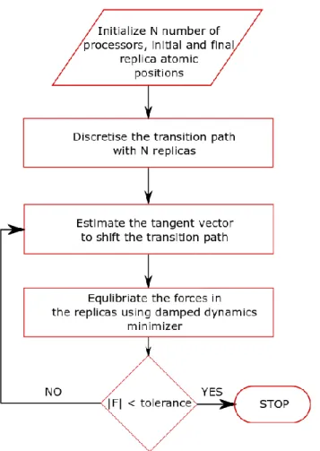
(32) Thèse de Srinivasan Mahendran, Université de Lille, 2018. Chapter 2. Model and methodology. 2.2.2 Nudged elastic band approach The nudged elastic band (NEB) is an efficient static method (Jónsson et al. 1998; Henkelman et al. 2000), which helps to find the minimum energy path (MEP) between two configurations corresponding to basins in the energy landscape. In this work we will use the NEB method to compute the Peierls potential associated with a glide event (Figure 2.4). For our case with large systems containing dislocations NEB saves computational time and resources in comparison with Hessian based methods. Since initial and final local minima are known in our case, the NEB is computationally efficient to trace the MEP.. Figure 2.4. Schematic representation of nudged elastic band calculation. Solid white balls in the 3D energy landscape represent the replicas. The initial and final replicas in the local energy minimum connected with other replicas using springs, the dashed line shows the initial guess and the solid line represents the minimum energy path.. The calculation of MEP using NEB method involves three major steps (Figure 2.5). Initially a discretised transition path is defined by creating R replicas, each replica representing a copy of the whole system. The replicas 1 and R are at initial and final local minima. In other words, they can be considered as reactant and product of a reaction 32 © 2018 Tous droits réservés.. lilliad.univ-lille.fr.
(33) Thèse de Srinivasan Mahendran, Université de Lille, 2018. Model and methodology. Chapter 2. respectively. The remaining, intermediate R-2 replicas contain the process path of the reaction. To prevent the replicas in the middle to move towards local minima during force minimization they are connected to each other using “springs” of unstretched length and spring constant k.. Figure 2.5. A simple flowchart to describe the shifting of initial guessed transition path towards MEP in a NEB calculation.. Firstly, the initial guess of the replicas in the reaction path are created using linear interpolation between the reactant and the product. Further, to reduce the force in the system the initial path is moved towards convergence by estimating the tangent vector to the path at each replica. The tangent vectors are determined to ensure better convergence in complex landscapes. Finally, the transition path is optimized by running the algorithm to move the replicas until forces in the system are below an expected force tolerance. The 33 © 2018 Tous droits réservés.. lilliad.univ-lille.fr.
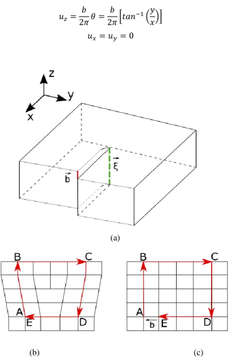
(34) Thèse de Srinivasan Mahendran, Université de Lille, 2018. Chapter 2. Model and methodology. replicas in the middle are not to be moved to local minima (i.e., energy minimized) during optimization, so the default Conjugate gradient or Steepest-descent minimization algorithms cannot be used in this process. In this work we use Quickmin algorithm a damped dynamics based minimization algorithm implemented in LAMMPS (Sheppard 2008).. 2.3 Dislocations modelling All real materials contain defects which may be classified as point, line, surface, and volume defects. These defects significantly alter the theoretical properties of crystalline solids. In this work, we focus on the type of line defect called dislocations which play a major role in the plastic deformation of solids. The concept of dislocation has been independently proposed by Orowan, Polanyi and Taylor in 1934. The discontinuity associated with a dislocation in a crystal can be well described using an atom to atom path drawn to form a closed loop around the defect, called the Burgers circuit. When the same loop is drawn in a perfect part of the same crystal, the circuit will not close. The closure vector is called the Burgers vector. Based on the Burgers vector direction respective to the dislocation line, dislocations can be classified in to two endmember types as screw and edge dislocations. The Burgers vector is parallel to the dislocation line for screw dislocations and perpendicular to the dislocation line for edge dislocations. The long-range displacement fields associated with dislocations can be described using continuum mechanics, whereas the elastic theory associated with this method fails near the dislocation core since the dislocation line represents a discontinuity in the displacement field. Hence, atomistic modelling of dislocation cores became an attractive tool to model dislocation cores which is an important component to understand intrinsic dislocations properties in particular lattice friction. At the atomic scale, one can start from the solution provided by the isotropic elastic theory (Hirth and Lothe 1968) to introduce dislocations in a system. For screw dislocations, as mentioned earlier, the Burgers vector b is parallel to dislocation line ξ (Figure 2.6.a). There are no addition or removal of atoms in the case of screw dislocations, Figure 2.6.b and c shows a typical example for creation of edge dislocation that involves the removal of 34 © 2018 Tous droits réservés.. lilliad.univ-lille.fr.
(35) Thèse de Srinivasan Mahendran, Université de Lille, 2018. Model and methodology. Chapter 2. atoms in a half plane. A displacement is applied to each atom along the z-direction. The magnitude of the displacement increases from zero to b based on the θ value of the displacement uz given as follows. 𝑢𝑧 =. 𝑏 𝑏 𝑦 𝜃= [𝑡𝑎𝑛−1 ( )] 2𝜋 2𝜋 𝑥. (2.17). 𝑢𝑥 = 𝑢𝑦 = 0. (2.18). (a). (b). (c). Figure 2.6. (a) A simple screw dislocation in created by “cut and slip” procedure. The slip or Burgers vector and the dislocation line are parallel to each other. (b) A simple cubic system containing edge dislocation represented using a Burgers circuit and (c) the same circuit represented in a perfect crystal. 35 © 2018 Tous droits réservés.. lilliad.univ-lille.fr.
(36) Thèse de Srinivasan Mahendran, Université de Lille, 2018. Chapter 2. Model and methodology. In case of an edge dislocation with a dislocation line ξ along the z-direction, the atoms are displaced along the x and y directions. For a material with a Poisson ratio 𝜈, the displacements applied to the atoms are as follows, 𝑢𝑥 =. 𝑏 𝑦 𝑥𝑦 [𝑡𝑎𝑛−1 ( ) + ] 2𝜋 𝑥 2(1 − 𝜐)(𝑥 2 + 𝑦 2 ). 𝑢𝑦 = −. 𝑏 𝑦 𝑥𝑦 [𝑡𝑎𝑛−1 ( ) + ] 2𝜋 𝑥 2(1 − 𝜐)(𝑥 2 + 𝑦 2 ). (2.19) (2.20). For simplicity, the isotropic expressions are given, however for the case of materials with lower symmetry in order to find the correct displacement field needed to move an atom from its position in the perfect crystal into its location in the dislocated crystal, we must turn to the anisotropic elastic theory. In general, for the case of more than two independent elastic constants, analytical solutions are not readily available and the displacement field must be found numerically (Steeds and Wills 1979). For a system containing straight dislocation analytical solutions equivalent to (2.18) – (2.20) are given by Steeds (Steeds 1973; Walker et al. 2005). The only advantage of using anisotropic elastic theory to insert a screw dislocation is to have a better starting point for atomic positions far from the dislocation core. Irrespective of the chosen elastic theory, the final dislocation core with anisotropic effects can be obtained after minimization of energy and forces in the system using pairwise potential. Since, the force fields used are intrinsically anisotropic. In this thesis, we limit our discussion to modelling of screw dislocations in forsterite. These displacements are introduced into the atomic system using an open-source program called ATOMSK (Hirel 2015). The ATOMSK code helps to create, modify and analyse the atomic systems. In case of screw dislocations, the major displacements are along the dislocation line (at least in the elastic theory description). Hence it is hard to visualize a screw dislocation, especially when viewed edge-on. For the purpose of visualizing screw dislocations, we use the differential displacement (DD) maps proposed by Vitek (1968). In this method, the relative displacements of neighbouring atoms due to the dislocation are represented using 36 © 2018 Tous droits réservés.. lilliad.univ-lille.fr.
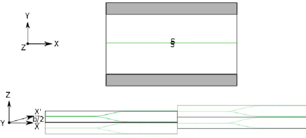
(37) Thèse de Srinivasan Mahendran, Université de Lille, 2018. Model and methodology. Chapter 2. arrows between them. The magnitude of an arrow is directly proportional to the magnitude of the difference in displacement between the two atoms. The magnitudes of the arrows are larger closer to the dislocation core centres.. Figure 2.7. Differential displacement plot of ½<111> screw dislocation core in BCC tantalum single crystal, plotted with respect to the displacement of neighbouring atom in oxygen sub-lattice. This picture is taken from Yang and Moriarty (2006).. 2.4 Atomistic modelling The basic problem with modelling dislocations using atomistic systems it that these defects have the long range field which cannot be truncated. This drawback can be solved by keeping maximum possible periodicity of the system. Simulations carried out in this work are performed using two types of simulation cells, the quasi-periodic slab type and the fully periodic quadrupole type. Both systems are built with a thickness equal to the Burger’s vector length, to simulate a straight, infinite dislocation line using periodic boundary conditions along the dislocation line.. 2.4.1 Slab type system Hirel et al. (2014) proposed a slab type geometry with a quasi-periodic boundary condition explained as follows. The dislocation line is introduced along the z-direction, and the direction of glide along the x-direction. The system is considered to be quasi-periodic since the periodicity is maintained along x and z directions, whereas along the y-direction the 37 © 2018 Tous droits réservés.. lilliad.univ-lille.fr.
(38) Thèse de Srinivasan Mahendran, Université de Lille, 2018. Chapter 2. Model and methodology. atoms at the top and bottom are frozen to replicate an infinite perfect crystal. The frozen zones help to prevent spurious elastic interaction between periodic replicas along y direction. With dislocation of Burgers vector b in the box, the periodic replicas along the x direction are matched by providing an additional tilt of b/2 along z as explained in Figure 2.8. The supercell is maintained long enough along the x direction to prevent dislocations interacting with their own periodic replicas, and the frozen zones are maintained far from each other along y direction. To reduce the effect of spurious interaction between periodic replicas, the box dimension is gradually increased to 480 Å and 140 Å along x and y Cartesian directions, respectively.. Figure 2.8. Schematic representation of “Slab” type geometry used in this work. The screw dislocation is introduced along the z Cartesian direction with glide plane along x direction. The b/2 tilt is added to the system to maintain the periodicity along x direction.. 2.4.2 Quadrupole system For ionic materials like forsterite, it is undesirable to have free surfaces, which can be charged. Hence, the periodic systems are preferred to model dislocations and their properties. The quadrupolar system is created by introducing four screw dislocations with two positive and two negative Burgers vectors along z-direction arranged simultaneously as shown in Figure 2.9. This alternate arrangement of dislocations of opposite Burgers vectors helps to lower the long-range elastic fields of the four dislocations (Lehto et al. 1998; Cai et al. 2004). This method helps to extract the dislocation core energies, to 38 © 2018 Tous droits réservés.. lilliad.univ-lille.fr.
(39) Thèse de Srinivasan Mahendran, Université de Lille, 2018. Model and methodology. Chapter 2. compute Peierls stresses and the energy barriers. The size effect due to the distance between dislocations can be reduced by increasing the box dimension proportionately along the x and y directions.. Figure 2.9. Schematic illustration of a quadrupole simulation cell with two positive and two negative screw dislocation arranged alternatively.. 2.5 Dislocation motion Plastic deformation of a crystal can result from the motion of dislocations. Here we restrict ourselves to the conservative motion of dislocations in their glide planes. To move a dislocation from one position to another, it has to overcome a potential barrier. In absence of thermal vibrations, the dislocation needs an external stress to overcome the potential barrier. The critical stress required to move a dislocation without assistance of thermal activation is called the Peierls stress. To move a dislocation with a Burgers vector b, the force F acting on the dislocation line ξ due to a local stress field σ can be described using the Peach-Koehler equation. 𝐹 = (𝜎. 𝑏) × ξ. (2.21). Based on the above relation, to trigger motion of a screw dislocation aligned with the zdirection to move along x direction, the system is loaded with εyz shear strain increments of 1%, ensuring quasi-static loading. After each increment the system is relaxed using a 39 © 2018 Tous droits réservés.. lilliad.univ-lille.fr.
(40) Thèse de Srinivasan Mahendran, Université de Lille, 2018. Chapter 2. Model and methodology. conjugate gradient minimization scheme. As a result, the stress in the system increases linearly. The stress-strain curve deviates from linearity for a critical stress at which the dislocation starts to move, defining the onset of the plastic regime. The critical stress at which the dislocation motion is observed defines the Peierls stress. This calculation is carried out using both simulation cells of quadrupole and slab type geometries. The calculations are repeated with gradual increase in simulation cell sizes along x, y directions to ensure independence with system size effects. NEB calculations are used to determine the Peierls potential VP as soon as the MEP is plotted with respect to the good reaction co-ordinate so in this case the dislocation core position. The Peierls potential represents the energy barrier that the dislocation has to overcome to move from one stable position to another. The Peierls stress associated with the motion can be computed from the maximum slope of the energy barrier. (. 𝑑𝑉𝑃 ) = 𝑏. σ𝑃 𝑑𝑥 𝑚𝑎𝑥. (2.22). In this work, the NEB calculations are performed using the THB1 pair potential via Quickmin damped dynamics minimization algorithm. The MEP are computed using 15 and 23 replicas which are connected to each other with springs having a spring constant of 0.1 eV/Å. To perform the damped dynamics minimization, shell model simulations are performed using adiabatic dynamics as suggested by Mitchell and Fincham (Mitchell and Fincham 1992). This involves allocating each shell a fraction of mass of its corresponding core and their motions integrated in the same way as that of the core, by integration of classical equations of motion. This method has been tested in simulations of various ionic materials and has been proved successful and computationally efficient (Mitchell and Fincham 1992; de Leeuw and Parker 1998; X.W. Sun et al. 2007, Yihui Zhang et al. 2009).. 40 © 2018 Tous droits réservés.. lilliad.univ-lille.fr.
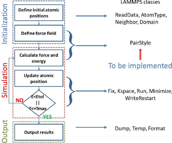
(41) Thèse de Srinivasan Mahendran, Université de Lille, 2018. Implementation and validation of THB1 potential library. Chapter 3. 3. Implementation and validation of THB1 potential library In the previous chapter we described the pairwise potential library with core-shell approximation used to model forsterite. In this chapter we will briefly discuss the implementation of a core-shell model potential library to a well parallelised open-source classical molecular mechanics package. After the algorithm for implementation, the energy and force fields implemented are validated by computing bulk properties of forsterite in comparison with first-principle calculations. The THB1 parametrisation is further validated by modeling non-equilibrium properties.. 3.1 LAMMPS dependencies LAMMPS is an acronym for Large-scale Atomic/Molecular Massively Parallel Simulator. LAMMPS is a classical molecular mechanics code (Plimpton 1995), developed at Scandia National Laboratory, a US Department of Energy Facility. It is an open-source code distributed under the GNU/GPL (General Public License). Initially the LAMMPS code was written in Fortran F77 and F90, whereas the present version of LAMMPS are developed in C++ with MPI message-passing library. Well optimized LAMMPS algorithm effectively runs simulations with systems containing few particles to millions. Hence, it can be used for model systems of various applications such as atomic, metallic, biological, granular and coarse-grained structures with the help of a variety of force fields and boundary conditions. To model dislocation core and its mobility with systems having few thousands of particles, a well parallelised and optimized code is necessary. We choose LAMMPS, because it is faster for large systems in comparison to the existing codes containing core-shell models (for instance GULP (Gale 1997)), thanks to effective neighbour list implemented in LAMMPS (Thompson et al. 2009; Plimpton and Thompson 2012) and the flexibility for developers to extend. The LAMMPS source code has been divided into various classes and the data are passed between them using pointers. The backbone of LAMMPS is constructed on a dozen of toplevel class, which are visible throughout the code (for example the atomic co-ordinates from Atom class). Next to these are a set of virtual parent classes, which LAMMPS defines 41 © 2018 Tous droits réservés.. lilliad.univ-lille.fr.
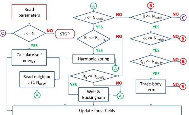
(42) Thèse de Srinivasan Mahendran, Université de Lille, 2018. Chapter 3. Implementation and validation of THB1 potential library. as “style”. The style classes contain the parameters and constraints that are imposed during a simulation. Each parent class holds a list of child classes, which the developers are expected to contribute to increase the capability of LAMMPS. In this work the THB1 potential library is implemented as a child class under a parent class called “Pair style”. The layers of the LAMMPS code and their different classes are illustrated in Figure 3.1.. Figure 3.1. Flowchart representation of structure of LAMMPS and classes in LAMMPS.. 3.2 Force fields This section explains about the implementation of core-shell library of inter-atomic potentials and their corresponding analytical forces into LAMMPS code. LAMMPS is designed in such a way to allow users to develop new potentials as class Pair styles without disturbing the core of the source code. The THB1 potential library consists of an 42 © 2018 Tous droits réservés.. lilliad.univ-lille.fr.
(43) Thèse de Srinivasan Mahendran, Université de Lille, 2018. Implementation and validation of THB1 potential library. Chapter 3. electrostatic term, a short-range Buckingham potential, a harmonic spring term and a threebody term. The expressions required for calculating force fields acting on every ion can be calculated from the negative gradient of the potential energy in equation (2.10). In summary, the force is calculated as, 𝑓 = −𝛻𝑈𝑇𝑜𝑡𝑎𝑙. (3.1). The force field of ions from Columbic interaction is computed using the Wolf summation method (Wolf et al. 1999), it is a spherically truncated, charge-neutralized pair potential which makes a 1⁄𝑟 summation. A cautious implementation of a self-energy term is carried out, to ensure that 𝑞𝑖𝑜𝑛 is the total charge of ion (i.e., charge of core and shell are not separately added to the self-energy term). The first derivative calculation for the electrostatic term is well discussed by Wolf et al. (1999). In summary, the final form of the electrostatic force term implemented is as follows, 𝑓𝐶𝑜𝑢𝑙𝑜𝑚𝑏 𝛼 𝑟𝑖𝑗𝛼 𝑒𝑟𝑓𝑐(𝛼𝑅𝑐 ) 2𝛼 𝑒𝑥𝑝(−𝛼 2 𝑟𝑖𝑗2 ) ( + ) × 𝑟𝑖𝑗 𝑟𝑖𝑗 𝑟𝑖𝑗2 𝜋 1⁄2 = ∑ 𝑞𝑖 𝑞𝑗 2 2 𝑟𝑖𝑗𝛼 𝑒𝑟𝑓𝑐(𝛼𝑅𝑐 ) 2𝛼 𝑒𝑥𝑝(−𝛼 𝑅𝑐 ) 𝑗≠𝑖 −( + ) × | 𝑅𝑐2 𝑅𝑐 𝑅𝑐 𝑟 𝜋 1⁄2 (𝑟𝑖𝑗 <𝑅𝑐 ) {. 𝑖𝑗 =𝑅𝑐. (3.2) }. Forces from short-range pair interaction between shells separated by a distance less than a user-defined cut-off of 𝑅𝐵 , is described by first derivative of two-body Buckingham potential 𝑈𝑆ℎ𝑜𝑟𝑡 from equation (2.12) is as follows, 𝑓𝑆ℎ𝑜𝑟𝑡 𝛼 = (−6𝐶𝑖𝑗 𝑟𝑖𝑗−6 +. 𝐴𝑖𝑗 𝑟𝑖𝑗 𝑟𝑖𝑗𝛼 𝑒𝑥𝑝 (− ) × 𝑟𝑖𝑗 ) × 2 , 𝑟𝑖𝑗 < 𝑅𝐵 𝐵𝑖𝑗 𝐵𝑖𝑗 𝑟𝑖𝑗. (3.3). The attraction force between the core and its corresponding shell is provided by the first derivative of the harmonic spring term with respect to the distance of separation between them 𝑟𝑖 , and the maximum distance between a core and its shell is given by a spring cut off term 𝑅𝑠𝑝𝑟𝑖𝑛𝑔 . 𝑓𝑠𝑝𝑟𝑖𝑛𝑔 𝛼 = − (𝐾1 +. 𝐾2 𝑟𝑖2 ) 𝑟𝑖𝛼 , 𝑟𝑖 < 𝑅𝑠𝑝𝑟𝑖𝑛𝑔 6. (3.4). 43 © 2018 Tous droits réservés.. lilliad.univ-lille.fr.
Figure

+7
Documents relatifs