How to value brands correctly?
A case study on adidasCharlotte Carpentier 28659
Under the supervision of Patrick Legland June 2014
Abstract
Brands are both seen as the most strategic assets of many firms, and the least identifiable when looking at financial statements, due to their absence from balance sheet (in case of non-acquisition). The main reason for that is that their valuation leads to high discrepancies depending on the valuator, the method used and the valuation date.
The objective of this study is to gather and classify the main brand valuation methods used by both academics and practitioners, before applying them to the practical case of adidas in order to isolate the one leading to apparently most accurate results compared to benchmark valuations from third parties.
Based on the study of adidas, we noted that even if the methods lead to very diverse results, the determination of a valuation range is still feasible to get a first idea of brand value. The methods leading to the most consensual results for the adidas case were the royalty relief approach and the demand driver approach, which are the ones mostly used by practitioners as stated by Salinas (2009). The attributes of methods leading to reasonable values seem to be having a mixed approach (both market-based and income-based), and being simple i.e. requiring neither many hypotheses nor deep delving into details. Nevertheless, the attribution of a precise figure is still difficult to rationalise, and mostly based on negotiation features or valuator’s perception of the brand.
Table of contents
Abstract ... 2
Introduction ... 5
I – A first step ... 6
1. Definition of the scope of analysis ... 6
2. Why to value brands? ... 7
II – Review of the main existing methods of brand valuation ... 8
1. Income-based / contribution methods – DCF-based approaches ... 10
1.1.How to choose the discount rate and the lifetime length of the DCF performed? ... 10
1.2.Royalty relief approach ... 13
1.3. Price/volume premium approach ... 17
1.4.Margins comparison ... 20
1.5. Excess cash flow method ... 22
2. Costs based methods ... 24
2.1. Historical costs of creation ... 24
2.2. Replacement costs ... 26
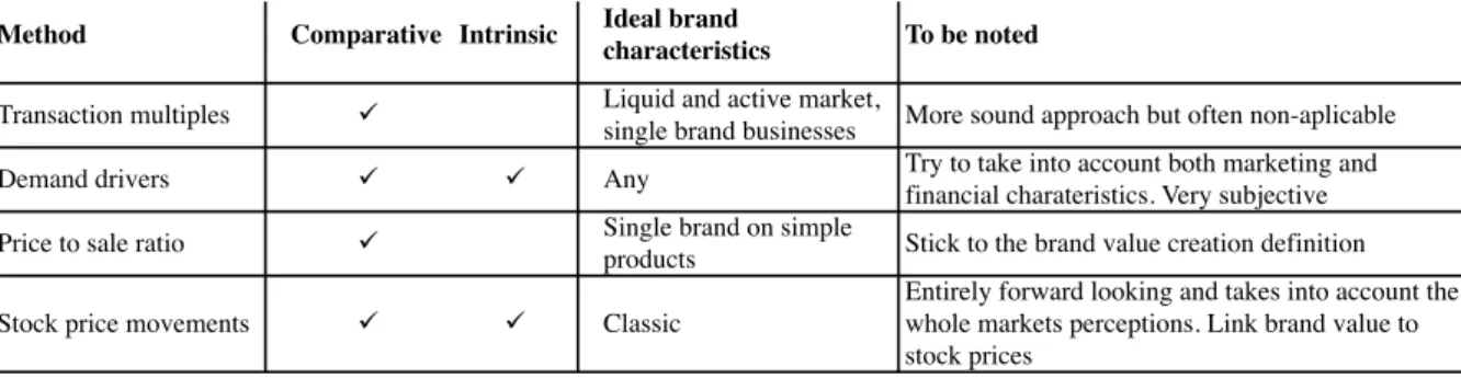
3. Market based methods ... 27
3.1.Transaction multiples ... 27
3.2. Demand driver/brand strength analysis ... 29
3.3. Differential of price to sales ratios ... 32
3.4. Stock price movements ... 34
4. Real options approach ... 36
4.1. General case ... 36
4.2. Pros, cons and key hypotheses in using this technique ... 39
5. Choosing the best method to use – a synthesis on the methods reviewed ... 40
III – A case study on Adidas – one brand, one value? ... 42
1. Why the choice of Adidas? ... 42
2. Business highlights - Brand history and strategy ... 42
Key information ... 42
Market penetration ... 44
Adidas brand SWOT analysis ... 44
Adidas AG financial elements ... 45
3. Valuation preliminary analyses ... 47
Common hypotheses ... 47
Company forecasts and WACC computation ... 48
Comparable “non-branded” firm ... 49
4. Adidas brand valuations ... 50
4.1. Benchmark valuations ... 50
4.2. Royalty relief method ... 51
4.3. Price premium method ... 53
4.4. Margin comparison method ... 55
4.5. Excess cash flow method ... 56
4.6. Historical costs method ... 58
4.7. Replacement costs method ... 58
4.8. Transaction multiple method ... 59
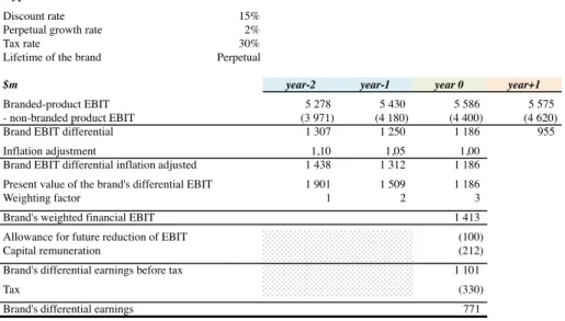
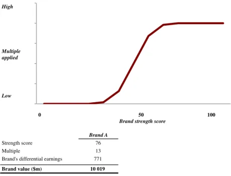
4.9. Demand driver approach ... 60
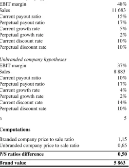
4.10. Price-to-sales difference ratio ... 64
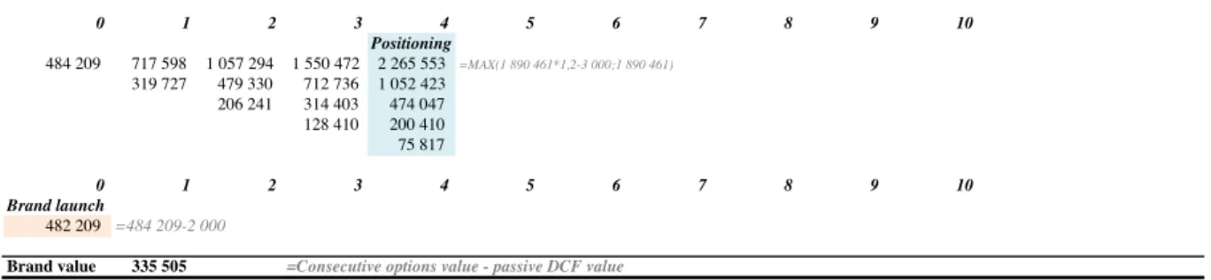
4.11. And what about considering real options? ... 66
5. Result comparisons and comments ... 72
Results summary ... 72
Attributes for a method to value brands correctly ... 77
6. Brand valuation: “An Art, not a science”? ... 78
Conclusion ... 79
References ... 80
Appendices ... 83
Appendix 1 – Adidas AG balance sheet – accounting view ... 83
Appendix 2 – Adidas AG 2013 Annual report – impairment on intangible assets ... 84
Appendix 3 – Market shares by geography ... 85
Introduction
“Intangible assets are recognized as highly valued properties. Arguably the most valuable but least understood intangible assets are brands”, states the ISO 10668 standard
(2010) in its introduction.
Brands are often seen as the most strategic intangible assets owned by a firm. What would Louis Vuitton bags be worth without the Louis Vuitton logo embroidered on them? Why are Starbucks coffees or Subway sandwiches so specific compared to simple basic coffees or sandwiches? Intuitively, anybody can perceive the value of a brand through its presence on TV screen, the story it tells, its innovations or its geographical presence.
Nevertheless, companies’ financial statements do not reflect at all this status: the most valuable brand according to Interbrand’s 2013 ranking1
, Apple, valued at $m 98 316, has total intangible assets on balance sheet 2
(September 28th
2013) of around $m 5 700. What is more, only few books cover this topic in deep detail; the major part of literature only tackling briefly the issue, presenting theoretical methods without delving into the problems raised by their application to real cases. Why do companies avoid valuing properly their brand in their financial statements? Why don’t analysts and markets ask for it, considering the high strategic aspect of this asset type?
A preliminary answer to these questions could be that brand valuation is too subjective to be called “valuation”. When looking at 2013 brand rankings by major third parties, the results speak for themselves: Apple is valued at $m 87 304 by BrandFinance, but at $m 185 071 by Millward Brown. McDonald’s is attributed a value of $m 90 256 by Millward Brown, and of $m 21 642 by BrandFinance. Valuing brands would thus seem to be arbitrary and results not reliable.
Taking into account the above considerations, the aim of this study is to review and classify the main existing brand valuation approaches, before applying them practically to the specific case of adidas. The objective is to highlight their limits in term of necessary inputs and result discrepancies; and to determine which methods seem to be the most accurate to value brands practically, based on public information.
1
http://www.interbrand.com/fr/ 2
Apple consolidated balance sheet - http://files.shareholder.com/downloads/AAPL/3030957356x0x701402/a406ad58-6bde-4190-96a1-4cc2d0d67986/AAPL_FY13_10K_10.30.13.pdf
I – A first step
1. Definition of the scope of analysis
Brands are part of our everyday life and may often be confused with the object or service they are attached to: who never used the term Kleenex for a tissue, Iphone for a phone?
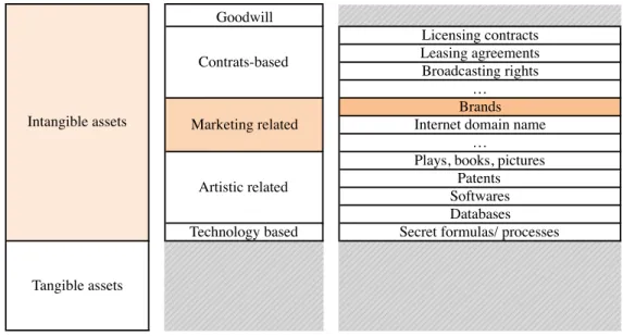
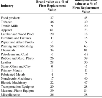
From a financial point of view, brands are part of intangible assets, as opposed to tangible ones, which mainly include real estate, production and technical equipment. Within the intangible assets side, they have to be distinguished from patents, buy-sell agreements, customer lists, specific rights (distribution rights, airport slots, domain rights), loans portfolios, permits, trade secrets etc. as shown in table 1.
The ISO 10668 standard (2010)3
, defines brands as “marketing-related intangible
assets including, but not limited to, names, terms, signs, symbols, logos, designs, or a combination of these, intended to identify goods, services and/or entities creating distinctive image and associations in the minds of stakeholders, generating economic benefits/values”.
The English law4
adds to this definition the “promise of an experience”, encompassing the quality, service and/or specific design the customer is expecting at buying the underlying asset. It adds that brands are above all “reputational” assets, based mainly on the beliefs of customers. Brands are thus not to be confused with possible other intangibles they support (e.g. patents in the case of a medicine brand like Doliprane). Salinas (2009) proposes three different scopes for brands definition:
- Name, logo and other visual elements;
- Name, logo, other visual and verbal elements and associated intellectual property rights;
3
ISO standards website - http://www.iso.org/iso/fr/home/store/catalogue_tc/catalogue_detail.htm?csnumber=46032 4
UK Intellectual Property Office - http://www.ipo.gov.uk/types/tm/t-about/t-whatis/t-brands.htm
Goodwill Licensing contracts Leasing agreements Broadcasting rights … Brands Internet domain name
…
Plays, books, pictures Patents Softwares Databases Technology based Secret formulas/ processes
Source: OECD study – Valuation of intangibles under IFRS 3R, IAS 36 and IAS 38, Jim Eales (2011)
Table 1 - Locating brands in a balance sheet
Tangible assets Intangible assets
Contrats-based
Artistic related Marketing related
- Organisational brand: this is the broader definition, referring to the organisational aspects of the brand and to what we will call later branded companies or businesses.
Only the first two scopes will be considered for the rest of the study.
Valuing brands correctly would thus mean putting a number on a marketing object with no material existence and more specifically on the future economic performance it is expected to generate. It thus has to be noted that the objective of this study is to discuss the valuation of brands as assets, and not the valuation of branded businesses as a whole, or of other assets possibly attached to but different from the concerned brands.
By valuing correctly, we mean:
- Estimating a fair value for the brand. Fair value is defined by IFRS 13 standard as the price that would be paid should the asset valued be transferred from an entity to another in a transaction. It is thus considered as the objective price for an asset, and may not coincide with the market price, which can sometimes include discounts or premiums. As for the ISO 10668 standard, it implies estimating the value of future economic advantages unlocked by the ownership of the brand, for its estimated lifetime. Consequently, we will only consider valuation methods allowing the estimation of an absolute monetary value for the brands, excluding thus methods estimating brands values relatively to one another.
- Appraising the best methods to be used and the way to apply them to reach the first point, among the existing methods, for the specific case chosen.
2. Why to value brands?
In financial statements, low or no information is given on the economic value of brands. Book value often misrepresents it. Indeed, according to IFRS 385
, brands developed internally should not be registered in balance sheet. Only brands acquired externally are to be registered at cost of acquisition and impaired once a year if needed. The example of Apple given in introduction shows the gap between the estimated fair value of the brand and its book value.
As explained by Rita Chraïbi in La Revue des Marques6
, market capitalisation and its variations reflect, behind the market value of shares, the value of the firms underlying intangible assets.If we consider that the market capitalisation is a reliable measure of a firm’s equity value, the difference between market capitalisation and equity book value should capture a significant part of the value of intangible assets not properly registered in the books. Nevertheless, these intangible assets do not correspond exclusively to brands, they can refer to patents, human capital, growth perspectives, knowledge or any other intangible asset booked at a value lower than fair value or not booked at all. Simply looking at the stock price of a company cannot thus lead to a perfect brand valuation, but only to a ceiling value.
However, being able to compute the fair value of a brand is useful in many situations faced by a company. A firm needs to be able to put a number on the name for the following purposes (not exhaustive):
- To buy or sell a brand (Unilever selling Lipton for example), - To license or franchise it to a tier company (Subway, McDonalds), - When involved in a litigation, for tax purposes,
- For accounting compliance (impairment tests, purchase price allocation),
5
www.focusifrs.com 6
- For managerial purposes, to better understand the drivers of its success and adapt its marketing strategy.
To be able to do so, we will review in the second part of the thesis the main brand valuation methods developed by the existing literature.
II – Review of the main existing methods of brand valuation
« Adding a 30% premium to the value estimate of Coca Cola is not a sensible way of capturing the value of a brand name »
The uValue companion, Stern NYU School of Business7
A brand has no minimal value. As it is intangible, it cannot be liquidated and its value is thus very volatile. During any valuation attempt, one should keep in mind that brand value arise from the power it gives to a company to sell products at higher prices, in larger quantities, or to decrease operating costs.
According to the ISO 10668 standard, a correct brand valuation should include the analysis of marketing and legal parameters, on top of financial parameters.
Across the literature reviewed, three main types of approaches can be distinguished: - Methods based on income generated by the brand,
- Methods based on cost supporting the brand development, - Methods based on market views.
The fourth point presents an additional method used on top of previous methods: real options. In order to make easier the understanding of the computation process of each method, we applied theoretically the methods to a simplified case: company Alpha, selling luxury shoes. Alpha basic financial information is the following:
7 http://people.stern.nyu.edu/adamodar/pdfiles/uValue/uValuebook.pdf Hypotheses Tax rate 30% WACC 10%
Brand earnings discount rate 15% Perpetual growth 2% Table 2 - Alpha hypotheses
Income statement
ACTUAL FORECAST EXTRAPOLATION
!m 2012A 2013A 2014F 2015F 2016F 2017E 2018E 2019E 2020E 2021E 2022E 2023E
Revenues 10!694 11!683 12!307 12!588 12!884 13!088 13!415 13!751 14!094 14!447 14!808 15!178 COGS (1!500) (1!639) (1!726) (1!766) (1!807) (1!836) (1!882) (1!929) (1!977) (2!026) (2!077) (2!129) Marketing (500) (546) (575) (589) (602) (612) (627) (643) (659) (675) (692) (710) Distribution (800) (874) (921) (942) (964) (979) (1!004) (1!029) (1!054) (1!081) (1!108) (1!135) R&D (250) (266) (274) (278) (282) (285) (292) (299) (306) (314) (322) (330) Personnel (900) (983) (1!036) (1!059) (1!084) (1!101) (1!129) (1!157) (1!186) (1!216) (1!246) (1!277) Other (377) (607) (807) (878) (974) (1!027) (1!053) (1!079) (1!106) (1!134) (1!162) (1!191) Operating Costs (4!327) (4!915) (5!339) (5!511) (5!713) (5!840) (5!986) (6!136) (6!289) (6!446) (6!607) (6!773) EBITDA 6!367 6!768 6!968 7!077 7!171 7!248 7!429 7!615 7!805 8!000 8!200 8!405 Depreciation (926) (931) (1!060) (1!064) (1!062) (1!054) (1!092) (1!145) (1!200) (1!259) (1!323) (1!511) Amortisation (7) (251) (333) (336) (344) (351) (359) (367) (375) (383) (392) (402) EBIT 5!434 5!586 5!575 5!677 5!765 5!843 5!978 6!104 6!231 6!358 6!485 6!492
Net Interest (Expense)/Income 0 0 0 0 0 0 0 0 0 0 0 0
Associates 0 0 0 0 0 0 0 0 0 0 0 0
Exceptionals (201) (200) 0 0 0 0 0 0 0 0 0 0
EBT 5!233 5!386 5!575 5!677 5!765 5!843 5!978 6!104 6!231 6!358 6!485 6!492
Taxes (1!570) (1!616) (1!673) (1!703) (1!729) (1!753) (1!794) (1!831) (1!869) (1!907) (1!946) (1!948)
Net Income 3!663 3!770 3!903 3!974 4!035 4!090 4!185 4!273 4!362 4!451 4!540 4!545
Average # Shares Outstanding (in '0 000) 8!667 8!675 8!675 8!675 8!675 8!675 8!675 8!675 8!675 8!675 8!675 8!675
EPS (EUR) 42,26 43,46 44,99 45,81 46,52 47,15 48,24 49,25 50,28 51,30 52,33 52,39
GROWTH
Revenues 9,2% 5,3% 2,3% 2,4% 1,6% 2,5% 2,5% 2,5% 2,5% 2,5% 2,5% EBITDA 6,3% 3,0% 1,6% 1,3% 1,1% 2,5% 2,5% 2,5% 2,5% 2,5% 2,5% EBIT 2,8% (0,2%) 1,8% 1,5% 1,4% 2,3% 2,1% 2,1% 2,0% 2,0% 0,1% Adj. Net Income
MARGINS
EBITDA 59,5% 57,9% 56,6% 56,2% 55,7% 55,4% 55,4% 55,4% 55,4% 55,4% 55,4% 55,4% EBIT 50,8% 47,8% 45,3% 45,1% 44,7% 44,6% 44,6% 44,4% 44,2% 44,0% 43,8% 42,8% EBT 48,9% 46,1% 45,3% 45,1% 44,7% 44,6% 44,6% 44,4% 44,2% 44,0% 43,8% 42,8% Net Income 34,3% 32,3% 31,7% 31,6% 31,3% 31,3% 31,2% 31,1% 30,9% 30,8% 30,7% 29,9% Source: Inspired by Naillon HEC Class
Table 3 - Alpha Income statement
Balance sheet
ACTUAL FORECAST EXTRAPOLATION
!m 2012A 2013A 2014F 2015F 2016F 2017E 2018E 2019E 2020E 2021E 2022E 2023E
Goodwill 3!189 2!989 2!989 2!989 2!989 2!989 2!989 2!989 2!989 2!989 2!989 2!989 Other Intangibles 4!165 4!004 3!758 3!503 3!237 2!959 2!685 2!415 2!150 1!890 1!635 1!385 PP&E 3!996 4!323 4!582 4!737 4!850 4!893 5!545 6!119 6!682 7!228 7!756 8!142
Financial Assets 5 5 5 5 5 5 5 5 5 5 5 5
Total Fixed Assets 11!355 11!321 11!334 11!234 11!081 10!846 11!224 11!529 11!826 12!112 12!385 12!521
Inventory 84 87 94 98 102 104 107 109 112 115 118 121
Accounts Receivable 943 1!060 1!143 1!192 1!239 1!271 1!303 1!335 1!369 1!403 1!438 1!474
Other Current Assets 0 0 0 0 0 0 0 0 0 0 0 0
Cash & Equivalents 1!016 4!198 7!453 10!860 14!390 18!060 21!232 24!550 27!951 31!438 35!013 38!716
Total Current Assets 2!043 2!333 8!690 12!150 15!731 19!435 22!642 25!995 29!432 32!955 36!569 40!311
Total Assets 13!398 13!654 20!024 23!384 26!812 30!282 33!866 37!524 41!258 45!068 48!954 52!832
Share Capital 11!086 11!086 11!086 11!086 11!086 11!086 11!086 11!086 11!086 11!086 11!086 11!086 Retained Earnings 387 3!608 6!945 10!334 13!773 17!258 20!829 24!474 28!195 31!991 35!863 39!727
Shareholders' Equity 10!094 10!330 18!031 21!420 24!859 28!344 31!915 35!560 39!281 43!077 46!949 50!813
Minority Interests 0 0 0 0 0 0 0 0 0 0 0 0
Provisions & Other Long-Term Liabilities 298 298 298 298 298 298 298 298 298 298 298 298
Financial Debt 0 0 0 0 0 0 0 0 0 0 0 0
Accounts Payable 497 544 565 536 525 510 523 536 549 563 577 591
Other Current Liabilities 1!130 1!130 1!130 1!130 1!130 1!130 1!130 1!130 1!130 1!130 1!130 1!130
Total Liabilities 3!304 3!324 1!993 1!964 1!953 1!938 1!951 1!964 1!977 1!991 2!005 2!019
Total Equity and Liabilities 13!398 13!654 20!024 23!384 26!812 30!282 33!866 37!524 41!258 45!068 48!954 52!832
Source: Inspired by Naillon HEC Class
Table 4 - Alpha Balance Sheet
Cash flow statement
ACTUAL FORECAST EXTRAPOLATION
!m 2012A 2013A 2014F 2015F 2016F 2017E 2018E 2019E 2020E 2021E 2022E 2023E
EBITDA 6!367 6!768 6!968 7!077 7!171 7!248 7!429 7!615 7!805 8!000 8!200 8!405
Cash Taxes (1!570) (1!616) (1!673) (1!703) (1!729) (1!753) (1!794) (1!831) (1!869) (1!907) (1!946) (1!948)
Net Interest (Expense)/Income 0 0 0 0 0 0 0 0 0 0 0 0
Intangibles Capex (85) (90) (87) (81) (78) (73) (85) (97) (110) (123) (137) (152) PP&E Capex (1!035) (1!258) (1!319) (1!218) (1!176) (1!097) (1!744) (1!719) (1!762) (1!806) (1!851) (1!897)
Change in NWC 92 (73) (69) (82) (62) (49) (22) (22) (23) (23) (24) (24)
Dividends from Associates / (to Minorities) 0 0 0 0 0 0 0 0 0 0 0 0
Other Cash Flow Items 0 0 0 0 0 0 0 0 0 0 0 0
Equity Free Cash Flow 3!769 3!731 3!820 3!993 4!126 4!276 3!785 3!946 4!042 4!141 4!243 4!384
Dividends 0 (549) (566) (585) (596) (605) (614) (628) (641) (654) (668) (681)
Change in Cash 3!769 3!182 3!255 3!407 3!530 3!671 3!172 3!318 3!401 3!487 3!575 3!703
Source: Inspired by Naillon HEC Class
1. Income-based / contribution methods – DCF-based approaches
The following table sums up the characteristics of the methods presented in this section.
1.1. How to choose the discount rate and the lifetime length of the DCF performed? Discount rate
The valuation methods presented in this section all use a DCF approach, by discounting to present value the cash flows or earnings assumed generated by the brand. Taking into account the brand specific risk and making the right assumption on the discount rate and lifetime length of the brand is thus necessary to avoid a significant under or overvaluation of the asset. We gather these two topics, common to the methods studied below, in this first point.
Despite the importance of choosing the right rate to use in such a valuation approach, this issue is not much covered in literature in the case of brands, and more broadly in the case of intangible assets.
BrandFinance® suggests to use an adjusted WACC to discount brand-related cash flows, computed as following:
!"#. !"## = !!∗ 1 − !! + !!+ !! ∗ 1 − !"# !"#$ ∗ !!
Where PD is the debt proportion in the whole business, Rf the risk-free rate, Ke the cost of
equity and Br the “brand risk premium”. This adjusted WACC is to be computed regionally to
take into account the difference in risk-free rate among countries and averaged to obtain the final adjusted WACC. Nevertheless, this approach seems approximate, particularly since the key point lies in how to determine Br. It thus seems to shift the issue on another variable, from
the rate of return to the risk premium.
Getting deeper into this topic, Schauten (2008) examines several suggestions in
Valuation, capital structure decisions and the cost of capital and recommends:
- Not to take the WACC to discount intangible cash flows: indeed, the risk of intangibles is, in the majority of cases, higher than the risk of the entire business;
- Not to take either the unlevered cost of equity as suggested by Smith and Parr. Even if intangibles are usually fund by equity only, this rate reflects as well the risk of the business as a whole and gives thus a wrong estimate of the required rate of return of intangible assets;
Method Comparative Intrinsic Ideal brand
characteristics To be noted
Royalty relief method ! ! Licensed or liquid market Most used approach Price/volume premium ! Single brand on simple
products Requires deep details within the companies figures Margin comparison ! Single brand on simple
products
Macro but potentially wrong view on the brand value creation
Excess cash flow ! In a company with few
other intangible assets Valuation by difference
- Avoid using the levered cost of equity, which charges the risk of debt on the intangible assets despite the fact that the debt was not raised to fund them. Nevertheless, he admits that the levered cost of equity being higher then the above two, it may be a better proxy of the required return on intangibles since the risk of these assets is, in many cases, higher than the risk of the company as a whole.
To solve the issue, Schauten recommends using the WARA method.
His whole model relies on the assumption that the weighted average cost of capital (WACC) is necessarily equal to the weighted average return on assets (WARA).
We thus have: !"## = !"#" !"## = !!"#∗ !"# ! + !+ !!" ∗ !" ! + !+ !!"∗ !" ! + !+ !!"∗ !" ! + ! !!" = !"## − (!!"#∗ !"#! + ! + !!"!"∗ !"! + ! + !!"∗ !"! + !) ! + ! Where:
- The WACC is computed as the weighted average of the cost of equity and the cost of debt before tax;
- WCR means Working Capital Requirement and !!"# is the return on WCR;
- TA means Tangible Assets and !!"is the return on tangible assets;
- IA means Intangible Assets and !!"is the return on intangible assets;
- TS means the present value of the tax Shield (i.e. the marginal tax rate multiplied by the value of debt) and !!"is the return on the tax shield (assumed equal as the cost of debt);
- Enterprise value = Equity value (E) + Debt value (D).
- The value of intangible assets IA is determined by difference between the market value of equity plus debt, and the other assets as booked in the financial statements (at market value if possible, at book value if not).
The rates of return on each asset class (WCR, tangible assets) may be either computed from internal data provided by the company owning the brand, or approximated using indexes (e.g. real estate index or leasing rate for tangible assets). The Canadian Institute of Chartered Business Valuators 8
sets boundaries on this issue, presenting the following diagram:
8
Note that Schauten’s method is based on Smith and Parr (2005) work, with an adjustment though: Smith and Parr use the WACC after corporate tax and do not formalize the tax shield as a separate asset, agglomerating it within intangibles, which, according to Schauten, leads to an underestimation of the required rate of return on intangibles.
Returning to brands, we think that the required rate of return on intangibles as above computed can be applied as a proxy for the required return on the brand studied. Theoretically, the split in asset classes done to compute this rate could be further investigated within the intangible assets, but finding rates of return for specific intangible assets other than the brand in order to compute the rate we are looking for by difference may become complicated (relying on many hypotheses) and unjustified.
On this topic, Salinas (2009) observe that the choice of the discount rate of brand earnings is one of the greater sources of conflict in brands valuation. Some practitioners use the related company’s WACC, others argue that the brands risk is lower than their sector’s risk. In the end, she notes that the discount rate is above all a matter of opinion; hence the diverse rates practically used and supposed to reflect the perceived brand’s risk.
To get an idea on how practically branded companies perceive their brand risk, one can approximate the discount rate to be used by the discount rate these companies report in their annual financial statements to impair goodwill and intangible assets. Hermès, for example, impairs its intangible assets using a rate of 10.5% in 2012, while stating in the same annual report a WACC of 10.14% considering thus the risk of its intangible assets as slightly higher than its WACC. On the contrary, Club Med in its 2013 annual reports does goodwill and intangibles impairments on the basis of its WACC (potentially to limit necessary impairment). These results illustrate the point of Salinas (2009): determining the right discount rate is “more an art than a science”.
Lifetime period
This question is a more subsidiary one since most brands are considered by practitioners to have an infinite lifetime. Nevertheless, some points highlighted by Salinas (2009) have to be taken into account.
The lifetime length of the brand to be taken into account in the DCF-based method should be its economic useful life, i.e. the time during which it creates value for the company
WACC WARA Discount rate Considerations
Superior to WACC Superior to Cost of Equity Highest Superior to return on other assets
RIS
K
High
Cost of Equity, in between rates for tangible asset backing and goodwill Lease rates
Low Mortgage rates
Asset-backed lending rates
Short-term borrowing rate Lowest
REWARD
Source: The Canadian Institute of Chartered Business Valuators - OECD TP WP6: Illustrative Example of Intangible Asset Valuation Table 7 - How to choose required rate of returns
Debt Equity Goodwill Intangible assets Fixed assets Working Capital
owning it. The following factors9
are thus to be analysed for any brand before concluding to an indefinite useful life:
- Life cycle of the product: fashion does not last forever;
- Functional obsolescence: it concerns particularly brands attached to lifestyle (slogans developed for short-term situations, product brands (i.e. Ipod, compared to Apple);
- Event obsolescence: failure of a company (e.g. Enron);
- Technological obsolescence: it concerns brands attached to technological innovations that may disappear following a disruptive entrance (e.g. well-known medicine);
- Cultural obsolescence: this factor may affect brands with non-politically correct names or concepts.
Once the discount rate and lifetime length discussed, one can tackle the remaining issues. The following subsections introduce the main income-based valuation methods, using the method presented here to compute the cash flows discount rate.
1.2. Royalty relief approach
Sources: Salinas (2009); Salinas and Ambler (2009); Brandfinance® (2013); PwC research
(2013), Husson and Philippe (Décideurs: Stratégie Finance droit n°92/93); Salinas (2009); Jucaityte and Virvilaite (2007)
1.2.1. General case
The royalty relief approach is the most commonly used for a technical valuation approach, according to Salinas and Ambler (2009)10
. Nevertheless, according to a PwC research 11
, it is used for intangibles of “second significance”. The general idea is to determine the brand-related cash flows by computing the fees a tier company would have to pay to use the brand without owning it. These fees are usually estimated as a percentage of the future sales of the licensor. The future estimated brand-related cash flows are then discounted to present value to get the brand value.
Deriving from the above definition, the main steps are the following: (1) Create a business plan for the whole company
As for any DCF valuation, the method is based on estimation of future firm’s revenues, relying on historical trends, market growth expectations and market share evolution. This step is supposed to partly embed the effects of the marketing strength of the brand.
(2) Determine the royalty rate to be applied
This is the key point of the method and potentially the most subjective.
According to Salinas (2009), it must be a function of the estimated brand strength, the duration of the brand (lifetime of agreements), the degree of exclusivity, the negotiating power of the firm in its industry, the product lifecycle, the firm’s local market environment (achievable margins), and the level of operating margins of the branded firm.
Several techniques are usually encountered:
9
Salinas (2009) – The International Brand Valuation Manual 10
Gabriella Salinas and Tim Ambler - A taxonomy on brand valuation practice: methodologies and purposes – April 2009 11
If the brand is already licensed, the access to the contractual agreement gives access to the real royalty fees invoiced. Nevertheless, these fees may not be composed only of the mere brand use rights but also of transfers of knowledge, material, and services enabling the licensee to comply with a certain level of quality expected by the customers for the concerned brand. In this case the main difficulty is to isolate the brand component.
If the brand is not licensed yet, we have to determine the would-be royalty rate from scratch, using peer tables. The royalty rate is determined based on a comparable approach, depending on the perceived strength of the brand, which includes both market positioning and intellectual protection. Within this method, authors make different recommendations. Brandfinance® (2013), in particular, recommends to choose comparable brands on criteria of similarities in margins and value drivers, to set an average value and a range of values (minimum and maximum) corresponding to the sector values, and to finally apply a multiplier (a percentage from 1% to 100% reflecting where the brand stands within the minimum-maximum range) to this rate, highlighting the brand specificities and strength12
. Others give less detail on how to select the right royalty rate, leaving more space to experience and judgement (e.g. average of comparable royalty rate, adjusted average). The Knoppe formula, as presented by Salinas (2009), gives guidelines and possibility to check the obtained result: it states that the royalty rate should be around 1/3 of the licensed product income divided by its sales.
(3) Determine the cash-flow discount rate and lifetime of the brand This point is developed in 1.1.
In the case of an infinite lifetime of the brand, we will need to determine a perpetual growth rate to compute the DCF terminal value. The literature reviewed does not give insights on how to choose this perpetual growth rate and thus lives this choice to the experience and judgment of the valuator. In this method we suggest the perpetual growth rate applied to be in line with the perpetual growth rate estimated for revenues in the business plan. Indeed, here, the brand cash flow growth is directly linked to the sales growth. The case of decreasing royalties over time is reviewed below in the Kern (1962) model. Perpetually increasing royalties, implying thus a perpetual growth rate of brand-related cash flows superior to the sales growth rate, are not credible over the long run since the brand necessarily reaches maturity at some point.
(4) Apply the following formula:
!"#$% !"#$% = !"#"$%"&!∗ !"#$%&# !"#$ ∗ (1 − !"# !"#$) (1 + !"#$%&'( !"#$)!
!
!!!
1.2.2. A specific case: the Kern x-times model (1962)
This model was initially developed by Kern (1962). As cited by Salinas (2009)13
, and Jucaityte and Virvilaite (2007)14, the underlying valuation mechanism is the same as for the general royalty relief model, with the estimation of future
12
This method, despite clearly using a royalty relief approach, may also be classified in the demand driver/brand strength analysis paragraph 13
The International brand valuation manual – Gabriela Salinas - 2009
14
revenues related to the ownership of the brand, discounted to present value. Additionally, Kern assumes that:
- The royalty revenues will increase in line with revenues but in a decelerating curve (hence the square root function in the formula below): the sales directly triggered by the brand will erode with the ageing of the brand,
- Brands have finite lifetime.
After some time, brands strength and royalty rates tend to decrease following a certain obsolescence of the brand.
The formula used is the following: !"#$% !"#$% = !! !∗ ! ∗ !!!!
!!∗(!!!) with ! = 1 + !
!"" and,
R: average expected annual revenues, L: Normal royalty rate in the industry, n: brand lifetime horizon,
q: annuity present value factor, p: country interest rate.
! =!!!∗(!!!)!!! is called the capitalisation factor.
Nevertheless, according to Zimmermann et al. (2001) as cited by Salinas (2009), no empirical study demonstrated the functional relationship chosen by Kern (i.e. the use of a root function) and the determination of n often remains arbitrary and subjective.
What is more, the finite lifetime of brand model cannot be applied to all types of brands: some brands having already existed for centuries, it may be complicated to choose the year in which they will stop existing, or to estimate what “indefinite” would mean for a brand (e.g. 100 years, 600 years).
The following table gives an example on how to apply the royalty relief method and the difference in results that can be obtained with the Kern model.
1.2.3. Pros, cons and key hypotheses in using this technique
Pros
The royalty relief technique and its derived methods allow for an obvious separation between the brand itself and its underlying asset (the rest of the company) through the definition of a rate rewarding only the extra profit generated by the brand. Through the royalty rate estimate, it also takes into account the industry environment in which the brand evolves, the target royalty rates being very different from one industry to another (from 1% to 10% according to Husson and Philippe).
This method is widely accepted by authorities since cited in the ISO 10668 standard15,
and can mostly be performed on publicly available information.
What is more, this approach reflects the commercial aspect of brands through a type of “renting” cost and recognizes the fact that a brand can be valuable in itself, even it is attached to a non-performing business (margins are indeed not taken into account). It also takes into account marketing and legal aspects on top of financial aspects, as recommended by the ISO standards.
Its subjectivity is a more discussed topic and depends on the information available: - If the brand is already licensed, the access to the fair royalty rate (with the necessary
analysis of its components) should be relatively easy,
- If the brand is not licensed, the estimation of the royalty rate is mainly based on comparable agreements appraisal and judgment, which is inherently more subjective.
15
Edouard Chastenet (April 2012) - Revue Française de comptabilité N°453 - Une norme international sur l’évaluation financière des marques: utilité pour les
préparateurs et les utilisateurs des états financiers
Hypotheses
Royalty rate 7%
Discount rate 15%
Tax rate 30%
Perpetual growth rate 2%
Lifetime of the brand Perpetual
Classic method
m! 2013 2014 2015 2016 2017 2018 2019 2020 2021 2022 2023
Year 0 1 2 3 4 5 6 7 8 9 10
Sales 11!683 12!307 12!588 12!884 13!088 13!415 13!751 14!094 14!447 14!808 15!178
Pretax royalty income 818 861 881 902 916 939 963 987 1!011 1!037 1!062
Taxes (245) (258) (264) (271) (275) (282) (289) (296) (303) (311) (319)
After taxes royalty income 572 603 617 631 641 657 674 691 708 726 744
Discount factor 0,933 0,811 0,705 0,613 0,533 0,464 0,403 0,351 0,305 0,265 0,231 Present value of royalty income 534 489 435 387 342 305 272 242 216 192 171 Sum of discounted royalty income (2013-2023) 3!585
Terminal value 1!345
Brand value (classic method) 4!930
Adaptation: Kern model
Complementary hypotheses
Lifetime of the brand (in years) 150
Country risk-free rate 2,5%
Computation
Annuity present value factor 1,0003
Capitalisation factor 147
Average expected annual revenue (13-23) 13!477
Brand value (Kern method) 5!835 Table 8 - Royalty relief method application example
Nevertheless, compared to other methods, it remains more objective since based on third parties agreements.
Cons
At the root of the method in itself, depending on the sector, it may be difficult to find any comparable licensing agreement or the comparable range may be too wide to be able to conclude wisely. Indeed, brands are, by definition, unique assets and are thus inherently difficult to compare with one another.
What is more, royalty rates used either directly or in a comparative way may:
- Include components other than the mere right to use the brand. In this case, a further analysis of the split of the royalty rate between each underlying component (know-how, material) may be needed, but not necessarily feasible for each comparable chosen.
- Exclude certain rights on the brand, not transferred from the owner to the licensee but that should be taken into account in the brand valuation.
Finally, a risk of undervaluation remains: when a company accepts to pay to license a brand on a specific or indefinite period for a given royalty rate, this company is expecting to make a higher profit than the expenses incurred to use the brand. The market royalty rate may thus be slightly under its fair value.
Key hypotheses
The royalty relief method is sensitive to the following hypotheses: - Royalty rate,
- The discount rate and lifetime period (the Kern model is highly sensitive to the latter), - The perpetual growth rate (if needed).
The other hypotheses needed are the following:
- The tax rate used (the effective tax rate paid by the company),
- The future revenues of the firm over a sufficient period of time (usually 5 to 10 years).
1.3. Price/volume premium approach
Sources: Salinas and Ambler (2009), Fernández (2001), Husson and Philippe (Décideurs: Stratégie Finance droit n°92/93), Tollington (1999)
1.3.1 General case
This method relies on the observation that for a similar product, a branded product sells more in volume and at a higher price than a non-branded product. The extra price paid and additional volume sold over the lifetime of the brand would thus represent the brand value added.
Deriving from the above definition, the main steps to determine the brand value are the following:
(1) Find a similar unbranded product.
(2) Compute the price difference between the branded product and the non-branded similar product and estimate how it will evolve over time.
If the branded company is selling only one branded product, the calculus is easily done as a simple subtraction. Nevertheless, it does not represent the majority of branded companies. In the most common case, the price difference has to be estimated statistically, e.g. as an average of the price differences for all the products sold. The initial price premium
has then to be derived in the future, depending on estimates on inflation, market share evolution, market growth, product mix etc.
(3) Apply this price difference on the volume of branded product sold over the future period studied.
The main difficulty here is to estimate future volumes as for a business plan, over a sufficient period of time, relying on historical trends, market growth expectations, and market share evolution. At this step, one could observe that the brand also triggers additional volumes compared to the situation in which the product sold would not be branded. In this case, the present value of the volume premium will be computed separately and added to the present value of the price premium to obtain the brand value (see below).
(4) Deduct from the above result the expenses related to the brand maintenance.
These expenses should include marketing expenses, but could also reflect the additional costs e.g. in raw material (highlighting difference in quality) or in personnel costs (showing for example handmade premium, or specific choice in production place).
(5) Determine the rate at which to discount the excess profit computed. This point is developed in 1.1.
In the case of an infinite lifetime of the brand, we will need to determine a perpetual growth rate to compute the DCF terminal value. The literature reviewed does not give insights on how to choose this perpetual growth rate and thus leaves this choice to the experience and judgment of the valuator. As for the royalty relief method, the expected perpetual growth rate on the company’s sales may serve as a proxy.
(6) Apply the following formula to obtain the present value of the estimated excess profit generated by the brand:
!"#$% !"#$% = (!"#$%&% !!− !"! !"#$%&% !! ∗ !!− !) ∗ (1 − !!"#) (1 + !"#$%&'( !"#!)! ! !!! !"#$% !"#$% = !"(!"#$% !"#$%&$) Where p: price V: volume sold
E: expenses related to brand maintenance rtax: branded company’s effective tax rate
n: brand lifetime horizon PV: present value.
If a volume premium is identified, i.e. if the brand allows the owning firm to sell more products, it has to be estimated and added to the price premium present value. In this case: !" = !" !"#$% !"#$%&$ + !" !"#$%& !"#$%&$ − !"(!!!"#"$%&' !"#!$%!%), where PV(price premium), PV(volume premium) and PV(additional expenses) are computed as following:
!" ! !"#$%&$ = (!"#$%&% !!− !"! !"#$%&% !! ∗ !"! !"#$%&% !!) ∗ (1 − !!"#) (1 + !"#$%&'( !"#$)!
!
!" ! !"#$%&$ = (!"#$%&% !!− !"! !"#$%&% !! ∗ !"#$%&% !!) ∗ (1 − !!"#) (1 + !"#$%&'( !"#$)! ! !!! !" ! = !!∗ (1 − !!"#) (1 + !"#$%&'( !"#$)! ! !!!
The objective in separating the additional expenses present value is to not double count them both in the price premium and in the volume premium.
This method is usually presented including only the price premium or only the volume premium, excluding the additional expenses effect. The more complete method presented here is the one described by Fernández (2001) as the “most correct method, from a conceptual
point of view”.
The following table gives an example of how to apply this method practically in a simple way. In the example taken, we assumed for the terminal value computation a perpetual growth rate of 1% on brand earnings, which is equal to the assumed inflation on branded product prices, and close to current economy inflation.
Hypotheses
Inflation on branded product mix prices 1,0%
Inflation on non-branded product mix prices 0,7%
Non-branded product volume growth rate 1,0%
Branded product volume growth rate 1,0%
Tax rate 30%
Discount rate 15%
Perpetual brand earnings growth rate 2,0% Lifetime of the brand Perpetual
m! 2013 2014 2015 2016 2017 2018 2019 2020 2021 2022 2023
Year 0 1 2 3 4 5 6 7 8 9 10
Branded product average price 10,0 10,1 10,2 10,3 10,4 10,5 10,6 10,7 10,8 10,9 11,0 Non-branded product average price 7,0 7,0 7,1 7,1 7,2 7,2 7,3 7,4 7,4 7,5 7,5
Price difference 3,0 3,1 3,1 3,2 3,2 3,3 3,3 3,4 3,4 3,5 3,5
Non branded product average volume sold 1!269 1!282 1!295 1!307 1!321 1!334 1!347 1!361 1!374 1!388 1!402 Price premium cash flows before tax 3!807 3!910 4!016 4!125 4!236 4!350 4!467 4!586 4!709 4!834 4!963 Taxes (1!142) (1!173) (1!205) (1!237) (1!271) (1!305) (1!340) (1!376) (1!413) (1!450) (1!489)
Price premium cash flows after tax 2!665 2!737 2!811 2!887 2!965 3!045 3!127 3!211 3!296 3!384 3!474
Branded product mix average volume 1!168 1!180 1!192 1!204 1!216 1!228 1!240 1!253 1!265 1!278 1!291 Non branded product average volume sold 1!269 1!282 1!295 1!307 1!321 1!334 1!347 1!361 1!374 1!388 1!402
Volume difference (101) (102) (103) (104) (105) (106) (107) (108) (109) (110) (111)
Branded product average price 10,0 10,1 10,2 10,3 10,4 10,5 10,6 10,7 10,8 10,9 11,0 Volume premium cash flows before tax (1!007) (1!027) (1!048) (1!069) (1!090) (1!112) (1!135) (1!158) (1!181) (1!205) (1!229) Taxes 302 308 314 321 327 334 340 347 354 361 369
Volume premium cash flows after tax (705) (719) (734) (748) (763) (779) (794) (810) (827) (843) (860)
Specific branded product marketing, distribution, R&D expenses (1!686) (1!770) (1!808) (1!848) (1!876) (1!923) (1!971) (2!020) (2!070) (2!122) (2!175) Difference in personnel cost (200) (202) (204) (206) (208) (210) (212) (214) (217) (219) (221) Difference in raw material expenses (225) (230) (234) (239) (244) (248) (253) (258) (264) (269) (274)
Expenses related to brand management (2!111) (2!201) (2!246) (2!293) (2!327) (2!381) (2!436) (2!493) (2!551) (2!610) (2!670) Taxes 633 660 674 688 698 714 731 748 765 783 801
Brand expenses cash flows after tax (1!478) (1!541) (1!572) (1!605) (1!629) (1!667) (1!705) (1!745) (1!785) (1!827) (1!869)
Brand earnings 482 477 506 534 573 600 627 655 684 714 745
Discount factor 0,933 0,811 0,705 0,613 0,533 0,464 0,403 0,351 0,305 0,265 0,231 Present value of brand earnings 450 387 357 328 305 278 253 230 209 189 172 Sum of discounted royalty income (2013-2020) 3!157
Terminal value 1!347
Brand value 4!504
1.3.2. Pros, cons and key hypotheses in using this technique
Pros
This method is seen as “theoretically attractive16
” because easily understood intuitively. What is more, the price differential computation tends to remove subjectivity. Cons
Nevertheless, from a practical point of view, it is difficult to find strictly similar unbranded products, except for some very simple products or raw material (e.g. sugar, coffee). In the other cases, the price difference may include slight differences not directly due to the brand (e.g. packaging, quality), which are difficult to isolate.
What is more, the price difference may not be homogeneous for every branded product sold under the same brand: for example, Burberry sells clothes but also bags, glasses etc.: how to fairly take this diversity into account? Estimating future products prices and mix over 5 or 10 years may be out of reach. It may also be complicated to justify and estimate the sustainability of the premium computed.
Additionally, differences in volume may be biased by the company’s size or recentness.
Finally, estimating the expenses directly related to the brand may be arduous since these expenses are not capitalised and are often drown in general expenses such as marketing etc. along decades. What is more estimating additional expenses related to quality or production place playing a role in brand strength requires a deep analysis of the company operations, not necessarily available to the public.
This method is thus complicated to apply correctly without relying on simplifying or unjustified hypotheses.
Key hypotheses
This method is sensitive to the following hypotheses:
- Comparable non-branded product chosen and thus estimated price and volume difference computed,
- The discount rate and lifetime period chosen, - The perpetual growth rate (if needed).
The tax rate used is the effective tax rate paid by the company.
1.4. Margins comparison
Sources: Salinas and Ambler (2009); Salinas (2009) 1.4.1. General case
This method is close from the price/volume excess premium but takes into account more extensively cost advantages or disadvantages of owning the brand (e.g. economies of scale). It consists in comparing the margins of the branded company with either (1) the one of an unbranded business selling a similar product, (2) an average of the ones of selected competitors. The margins compared can be either the gross margin or the EBIT margin.
The steps are the same as in the price/volume method but the idea here is to apply the margin differential to the branded product forecasted revenues for the brand lifetime defined. The formula used will thus be the following:
16
!"#$% !"#$% = (!"#$%&% !"#$%&%!− !"! !"#$%&% !"#$%&%! ∗ !!) ∗ (1 − !!"#) (1 + !"#$%&'( !"#$)!
!
!!!
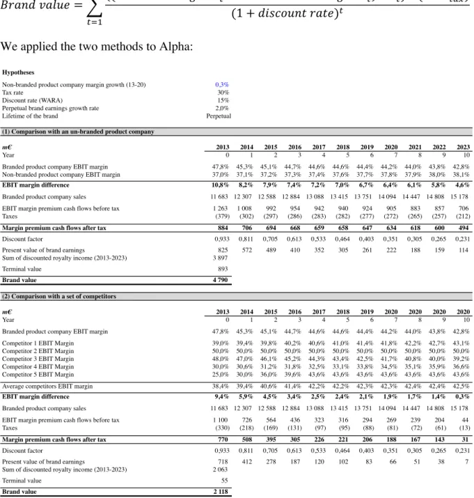
We applied the two methods to Alpha:
1.4.2. A derived case: marginal cash-flow comparison
This third approach is directly derived from the margins comparison but computing and discounting this time the difference between the free cash flows of a branded company and a non-branded company selling similar products.
1.4.3. Pros, cons and key hypotheses in using this technique
Pros
These three methods take more widely into account costs associated to the brand and are more easily applicable from publicly available information than the price/volume
Hypotheses
Non-branded product company margin growth (13-20) 0,3%
Tax rate 30%
Discount rate (WARA) 15%
Perpetual brand earnings growth rate 2,0% Lifetime of the brand Perpetual
(1) Comparison with an un-branded product company
m! 2013 2014 2015 2016 2017 2018 2019 2020 2021 2022 2023
Year 0 1 2 3 4 5 6 7 8 9 10
Branded product company EBIT margin 47,8% 45,3% 45,1% 44,7% 44,6% 44,6% 44,4% 44,2% 44,0% 43,8% 42,8% Non-branded product company EBIT margin 37,0% 37,1% 37,2% 37,3% 37,4% 37,6% 37,7% 37,8% 37,9% 38,0% 38,1%
EBIT margin difference 10,8% 8,2% 7,9% 7,4% 7,2% 7,0% 6,7% 6,4% 6,1% 5,8% 4,6%
Branded product company sales 11!683 12!307 12!588 12!884 13!088 13!415 13!751 14!094 14!447 14!808 15!178 EBIT margin premium cash flows before tax 1!263 1!008 992 954 942 940 924 905 883 857 706 Taxes (379) (302) (297) (286) (283) (282) (277) (272) (265) (257) (212)
Margin premium cash flows after tax 884 706 694 668 659 658 647 634 618 600 494
Discount factor 0,933 0,811 0,705 0,613 0,533 0,464 0,403 0,351 0,305 0,265 0,231 Present value of brand earnings 825 572 489 410 352 305 261 222 188 159 114 Sum of discounted royalty income (2013-2023) 3!897
Terminal value 893
Brand value 4!790
(2) Comparison with a set of competitors
m! 2013 2014 2015 2016 2017 2018 2019 2020 2020 2020 2020
Year 0 1 2 3 4 5 6 7 8 9 10
Branded product company EBIT margin 47,8% 45,3% 45,1% 44,7% 44,6% 44,6% 44,4% 44,2% 44,0% 43,8% 42,8% Competitor 1 EBIT Margin 39,0% 39,4% 39,8% 40,2% 40,6% 41,0% 41,4% 41,8% 42,2% 42,7% 43,1% Competitor 2 EBIT Margin 50,0% 50,0% 50,0% 50,0% 50,0% 50,0% 50,0% 50,0% 50,0% 50,0% 50,0% Competitor 3 EBIT Margin 48,0% 47,0% 46,1% 45,2% 44,3% 43,4% 42,5% 41,7% 40,8% 40,0% 39,2% Competitor 4 EBIT Margin 30,0% 30,6% 31,2% 31,8% 32,5% 33,1% 33,8% 34,5% 35,1% 35,9% 36,6% Competitor 5 EBIT Margin 25,0% 30,0% 36,0% 39,6% 43,6% 43,6% 43,6% 43,6% 43,6% 43,6% 43,6% Average competitors EBIT margin 38,4% 39,4% 40,6% 41,4% 42,2% 42,2% 42,3% 42,3% 42,4% 42,4% 42,5%
EBIT margin difference 9,4% 5,9% 4,5% 3,4% 2,5% 2,4% 2,1% 1,9% 1,7% 1,4% 0,3%
Branded product company sales 11!683 12!307 12!588 12!884 13!088 13!415 13!751 14!094 14!447 14!808 15!178 EBIT margin premium cash flows before tax 1!100 726 564 436 323 316 294 269 239 204 44 Taxes (330) (218) (169) (131) (97) (95) (88) (81) (72) (61) (13)
Margin premium cash flows after tax 770 508 395 305 226 221 206 188 167 143 31
Discount factor 0,933 0,811 0,705 0,613 0,533 0,464 0,403 0,351 0,305 0,265 0,231 Present value of brand earnings 718 412 278 187 120 102 83 66 51 38 7 Sum of discounted royalty income (2013-2023) 2!063
Terminal value 55
Brand value 2!118
premium approach developed above, which requires more detailed financial and operational information.
Compared to the price/volume premium approach, it seems to solve the product mix problem by considering blended margins / free cash flows.
Cons
A side effect of the advantage above described is that the EBIT margin and free cash flow include expenses not related to the brand ownership, which leads to undervaluation of the brand. On the contrary, gross margin may exclude some expenses directly related to the brand and lead to overvaluation. Looking at the brand from a more macroeconomic point of view is thus easier but necessarily leads to errors.
What is more, as for the price/volume premium approach, from a practical point of view, it may be difficult to find strictly similar unbranded products, except for some very simple products or raw material (e.g. sugar, coffee). This method adds difficulties if the company is selling products under different brands: the valuator has to analyse more deeply the product mix to create a representative blended margin. The alternative method suggesting to use competitors’ margins does not really isolate the brand but values the brand studied relatively to the brands of the competitors. It thus does not lead an absolute value. The example computed shows indeed that the second method leads to a much lower brand value, explained by the fact that it is the brand value on top of the value of average competitors brands.
Finally, it may be complicated to justify and estimate the sustainability of the margins/free cash flow computed.
These derived methods are thus complicated to apply correctly. Key hypotheses
These methods are highly sensitive to the comparable non-branded company chosen and thus estimated forecasted gross margin/EBIT margins/free cash flow.
The following hypotheses also affect the final brand value: - The discount rate and the lifetime period (see 1.1.);
- The perpetual growth rate (if needed).
The tax rate used is the effective tax rate paid by the branded company.
1.5. Excess cash flow method
Sources: Salinas and Ambler (2009), Fernández (2001), The Canadian Institute Chartered
Business Valuator (OECD TP WP6)
1.5.1 General case
This approach is still a DCF approach but the free cash flows attributable to the brand are computed here as the estimated free cash flows to firm from which are deducted for each year the estimated return of other assets not corresponding to the brand, i.e. the “assets
employed multiplied by the required return17
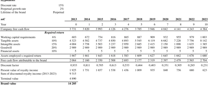
”. The table below, adapted from Fernández paper (2001) gives a practical example.
17
In this method, company free cash flow and assets employed are estimated based on a business plan considering historical trends, market growth expectations, market share evolution etc. Neither Fernández (2001) nor Salinas and Ambler (2009) give insights on how to fairly estimate the required return on each asset employed type. The WARA method developed in 1.1 may be applied to partly solve this issue.
This approach is in fact very similar to the marginal cash flow comparison method, but replaces the cash flows from a non-branded product company by the cash flows supposed to be dedicated to serving the assets employed different from the brand, the remaining cash flows being supposed to be related to the brand earnings.
1.5.2. Pros, cons and key hypotheses in using this technique
Pros
The issue of relying on comparable non-branded products disappears here since the method is totally concentrated on the company owning the valued brand.
Cons
The reliability of the whole method relies on the possibility to fairly estimate assets employed required returns excluding the brand, which shifts the issue of brand valuation to the issue of analysing the other company’s assets. The valuation is thus done by eliminating what composes the company’s value, without really focussing on the brand in itself. As a consequence, it is practically applicable only for companies owning a single brand. What is more, since this approach calculates the brand value by difference, there is a risk of overvaluation or undervaluation by wrongly attributing by omission some revenues or expenses to the brand. Excess in cash flow may not necessarily be due to the brand but to wrongly estimated required returns on the other assets identified, or to an unidentified asset.
Applying the same required returns for each asset class along the business plan may not reflect the reality of the business evolution. On the contrary, estimating the evolution of each category return would require an additional level of judgment, and would bring up the issue of how to choose the level of return to apply in the terminal value.
Finally, this method does not take at all into account marketing or legal aspects of the brand since it values it entirely from internal information.
Hypotheses
Discount rate 15% Perpetual growth rate 2% Lifetime of the brand Perpetual
m! 2013 2014 2015 2016 2017 2018 2019 2020 2021 2022 2023
Year 0 1 2 3 4 5 6 7 8 9 10
Company free cash flow 3!731 3!820 3!993 4!126 4!276 3!785 3!946 4!042 4!141 4!243 4!384
Required return
Working capital requirements 6% 603 672 754 816 865 887 909 932 955 979 1!003 Tangible assets 10% 4!323 4!582 4!737 4!850 4!893 5!545 6!119 6!682 7!228 7!756 8!142 Intangible assets 15% 4!004 3!758 3!503 3!237 2!959 2!685 2!415 2!150 1!890 1!635 1!385 Goodwill 20% 2!989 2!989 2!989 2!989 2!989 2!989 2!989 2!989 2!989 2!989 2!989
Financial assets 10% 5 5 5 5 5 5 5 5 5 5 5
Assets employed x required return 1!667 1!661 1!643 1!618 1!583 1!609 1!627 1!645 1!662 1!678 1!680 Free cash flow attributable to the brand 2!064 2!160 2!350 2!508 2!693 2!177 2!319 2!397 2!479 2!565 2!704 Discount factor 0,933 0,811 0,705 0,613 0,533 0,464 0,403 0,351 0,305 0,265 0,231 Present value of royalty income 1!925 1!751 1!657 1!538 1!436 1!009 935 840 756 680 623 Sum of discounted royalty income (2013-2023) 9!315
Terminal value 4!890
Brand value 14!205
Source: Adapted from Fernández (2001) citing Houlihan Valuation Advisors
Key hypotheses
This method is highly sensitive to the following hypotheses:
- Estimated forecasted free cash flow and assets employed (split and numerical estimates); - Required returns on each type of asset employed.
The following hypothesis also affects the final brand value:
- The discount rate (see 1.1.) and the lifetime period of the brand; - The perpetual growth rate (if needed).
2. Costs based methods
Sources: The Canadian Institute Chartered Business Valuator (OECD TP WP6), Husson and
Philippe (Décideurs: Stratégie Finance droit n°92/93), Tollington (1999), Anson, Noble and Samala (2014), Salinas and Ambler (2009)
“The value of an object or piece of intellectual property is no greater than the cost to
acquire that asset elsewhere, whether the cost of obtaining the asset is measured by purchasing it today or replacing it with a substitute asset of equal strength and utility”.18
The underlying idea of the methods presented below is thus that an external acquirer would not pay more than what it would cost him or her to recreate or find a substitute to the brand.
The following table sums up the characteristics of the methods presented in this section.
2.1. Historical costs of creation 2.1.1 General case
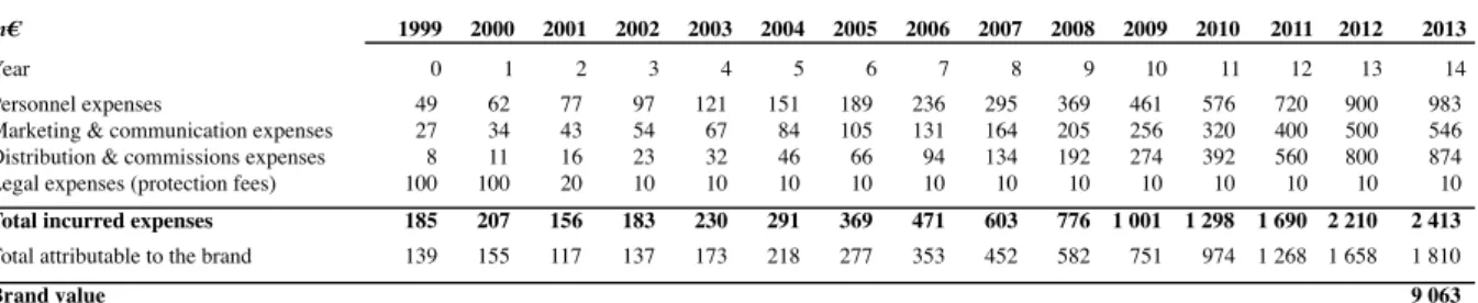
This method suggests that the value of a brand is the sum of the costs that have been incurred by the owning company to create the asset.
Three types of costs have to be taken into account: - “Hard costs19
”, which include any material or asset needed to build the brand; - “Soft costs20
”, designating intellectual work related to the brand such as time for design or engineering;
- “Market costs21
”, including all marketing and communication costs for advertising and more generally building the brand strength in its market.
To these accounting costs have to be added any opportunity costs such as a delay in entrance on market; and withdrawn any obsolescence factors (e.g. if the brand has a finite lifetime, the years already spent have to be taken into account) or restriction factors (e.g. due to the legal environment in which the brand is developed). The Canadian Institute Chartered
18
Anson, Noble and Samala (2014) 19
Anson, Noble and Samala (2014) 20
Anson, Noble and Samala (2014) 21
Anson, Noble and Samala (2014)
Method Comparative Intrinsic Ideal brand
characteristics To be noted
Historical costs ! Embryonic brand Gives a floor value
Replacement costs ! Embryonic brand More sound but more subjective and freely applied