Opetopes: Syntactic and Algebraic Aspects

(1)

HAL Id: tel-02968939

https://hal.archives-ouvertes.fr/tel-02968939

Submitted on 16 Oct 2020

HAL is a multi-disciplinary open access archive for the deposit and dissemination of sci-entific research documents, whether they are pub-lished or not. The documents may come from teaching and research institutions in France or abroad, or from public or private research centers.

L’archive ouverte pluridisciplinaire HAL, est destinée au dépôt et à la diffusion de documents scientifiques de niveau recherche, publiés ou non, émanant des établissements d’enseignement et de recherche français ou étrangers, des laboratoires publics ou privés.

Distributed under a Creative Commons Attribution - NonCommercial| 4.0 International License

Opetopes: Syntactic and Algebraic Aspects

Cédric Ho Thanh

To cite this version:

Cédric Ho Thanh. Opetopes: Syntactic and Algebraic Aspects. Category Theory [math.CT]. Univer-sité de Paris, 2020. English. �tel-02968939�

(2)

Opetopes

syntactic and algebraic aspects

A doctoral thesis written by

Cédric Ho Thanh

under the direction of

Prof. Pierre-Louis Curien, Université de Paris

and

Prof. Samuel Mimram, École Polytechnique

and submitted in fulfillment of the requirements for the degree of Doctor of Science in Mathematics

at Université de Paris (Denis Diderot),

doctoral school 386 “Sciences mathématiques de Paris centre”

Publicly defended on Thursday October 15th_{, 2020,} before a thesis jury comprised of

Denis-Charles Cisinski,Universität Regensburg president

Nicola Gambino,University of Leeds referee

Marek Zawadowski,Uniwersytet Warszawski referee

Eugenia Cheng, School of the Art Institute of Chicago member

Geoffroy Horel, Université Paris 13 member

François Métayer, Université Paris Nanterre member

Pierre-Louis Curien,Université de Paris director

(3)

(4)

Abstract

Opetopes are shapes (akin to globules, cubes, simplices, dendrices, etc.) intro-duced by Baez and Dolan to describe laws and coherence cells in higher-dimensional categories. In a nutshell, they are trees of trees of trees of trees of... These shapes are attractive because of their simple nature and easy to find “in nature”, but their highly inductive definition makes them diﬀicult to manipulate eﬀiciently.

This thesis develops the theory of opetopes along three main axes. First, we give it clean and robust foundations by carefully detailing the approach of Kock–Joyal– Batanin–Mascari, based on polynomial monads and trees. Starting with the identity functor on sets, and repeatedly applying the Baez–Dolan construction, we obtain a sequence of polynomial monads whose operations are trees over previous monads. This process generates opetopes and captures their recursive nature. We then introduce the important formalism of higher addresses, which allows to “walk” through opetopes and all their lower-dimensional faces simultaneously, in order to reach a given node or edge. This allows a more thorough investigation of the structure of the generating polynomial monads, and gives us important insights on the tree calculi they encode, in this case the natural operations on opetopes, such as grafting and substitution.

The second part of this thesis deals with computerized manipulation of opeto-pes. We introduce two syntactical approaches to opetopes and opetopic sets. In each, opetopes are represented as syntactical constructs whose well-formation conditions are enforced by corresponding sequent calculi. In the first one, called the named ap-proach, we express the compositional nature of opetopes using a specifically crafted kind of term. In the second, called unnamed approach, we just give a syntactical ac-count of the tree structure of opetopes using higher addresses. This latter approach is closer to the definition of the first part of this thesis, whereas the former is more human-friendly.

Lastly, in the third part of this thesis, we focus on the algebraic structures that can naturally be described by opetopes. So-called opetopic algebras include categories, planar operads, and Loday’s combinads over planar trees. We start by extending the generating polynomial monads to categories of truncated opetopic sets, and let opetopic algebras be simply algebras over these extensions. Later, we introduce the category of opetopic shapes, and using the theory of parametric right adjoint monads of Weber, we show that opetopic algebras can also be understood as presheaves over opetopic shapes having the unique lifting property against a certain set of maps. We then turn our attention to the notion of weak opetopic algebras and their homotopy theory. Following the literature in the simplicial and dendroidal cases, we introduce three models: ∞-opetopic algebras, complete Segal spaces, and homotopy-coherent opetopic algebras. We show that classical results of Rezk, Joyal–Tierney, and Horel (for ∞-categories), and Cisinski–Moerdijk (for ∞-operads) can be reformulated and generalized in our setting. In particular, these models are equivalent.

Keywords. Opetope, opetopic set, polynomial monad, polynomial tree, Baez–Dolan construction, sequent calculus, opetopic category, opetopic algebra, operad, combinad.

(5)

Résumé

Les opétopes sont des formes (tout comme les globes, les cubes, les simplex, les dendrex, etc.) inventées par Baez et Dolan afin de pouvoir décrire les cellules de co-hérence des catégories supérieures faibles. Informellement, ce sont des arbres d’arbres d’arbres d’arbres... Ces formes sont séduisantes car elles sont intrinsèquement simples et apparaissent fréquemment en pratique. Cependant, leur nature inductive les rend diﬀicile à manipuler eﬀicacement.

Cette thèse développe la théorie des opétopes selon trois axes. Premièrement, nous formulons une définition propre et robuste, en suivant minutieusement l’approche de Kock–Joyal–Batanin–Mascari, basée sur la théorie des monades et des arbres poly-nomiaux. En itérant la construction de Baez–Dolan sur le foncteur identité sur la catégorie des ensembles, nous obtenons une suite de monades polynomiales, et leurs opérations sont des arbres sur des monades précédentes. Ce processus génère les opé-topes et cerne leur structure récursive. Ensuite, nous présentons la notion d’adresse supérieure, qui nous permettent de “naviguer” dans les opétopes et leurs faces afin d’atteindre un nœud ou une arrête donné. Ce formalisme permet une étude plus poussée de la structure des monades polynomiales et des opérations sur les arbres qu’elles encapsulent. Dans notre cas, il s’agit des opérations naturelles sur les opé-topes, par exemple les greffes et les substitutions.

Ensuite, nous introduisons deux systèmes syntaxiques pour décrire les opétopes et les ensembles opétopiques, avec pour objectif leur implémentation informatique. Dans chacune de ces deux approches, les opétopes sont encodés par des expressions dont la validité est assurée par des calculs des séquents correspondants. Dans la première, appelée approche nommée, nous décrivons la structure compositionnelle des opétopes en utilisant un certain type de terme. La seconde, appelée approche anonyme, se con-centre sur une représentation syntaxique simple des arbres sous jacents aux opétopes. Bien que plus proche de la définition polynomiale, sa syntaxe est moins facile à lire que celle de l’approche nommée.

Enfin, dans la dernière partie de cette thèse, nous étudions les structures al-gébriques que les opétopes décrivent. Ces structures, que nous appelons algèbres opé-topiques, généralisent les catégories, les opérades planaires, et les combinades des arbres planaires de Loday. Nous commençons pas étendre les monades génératrices à des catégories d’ensemble opétopiques tronqués, de sorte à ce que les algèbres opé-topiques ne soient simplement que des algèbres sur ces extensions. Nous introduisons la catégories des formes opétopiques, et en mettant à contribution la théorie des ad-joints à droite paramétriques de Weber, nous montrons que les algèbres opétopiques peuvent se comprendre comme des préfaisceaux satisfaisant certaines conditions de relèvement unique. Nous nous intéressons ensuite à la notion l’algèbre faible. En se basant sur les théories existantes dans le cas simplicial et dendroïdal, nous en don-nons trois interprétations: les ∞-algèbres opétopiques, les espaces de Segal complets, et les algèbres opétopiques à homotopies cohérentes près. Nous montrons que certains résultats classiques de Rezk, Joyal–Tierney, et Horel (pour les ∞-catégories), et de Cisinski–Moerdijk (pour les∞-opérades) peuvent être reformulés et généralisés dans ce cadre. En particulier, ces trois modèles sont équivalents.

Mots-clefs. Opétope, ensemble opétopique, monade polynomiale, arbre polynomial, construction de Baez–Dolan, calcul de séquent, catégorie opétopique, algèbre opé-topique, opérade, combinade.

(6)

Introduction

H

igher structures appear increasingly in a variety of contexts, such as mathemat-ical physics, algebraic topology, knot theory, and representation theory, with the aim of providing finer and finer invariants for the objects under study, like spaces or groups. They arise naturally when weakening structures, for example relaxing a binary operation that is associative (typically, a category) into one where associativ-ity holds only up to homotopy (typically, a bicategory). One then needs to consider the homotopies between homotopies etc., and what coherence laws need to be enforced.

This thesis takes place in one of the formalisms that have been proposed to define such higher structures: the opetopes and opetopic sets of Baez and Dolan [BD98], further studied by Cheng [Che03a] [Che04b], Leinster [Lei04], Kock et. al. [KJBM10], and others. Opetopes are shapes (akin to cubes, globules, simplices, etc.) originally introduced to describe laws and coherence in higher category theory. Their name reflects the fact that they encode the possible shapes for higher-dimensional operations: they are operation polytopes. More concretely, while commutative diagrams (e.g. commutative squares) are a convenient representation of relations in 1-categories, and commutative squares with 2-cells for 2-categories, opetopes provide a formal account of pasting diagrams of cells in every dimension.

TOWARDS HIGHER STRUCTURES

Let us take a leisurely dive into a classical example of higher structure. Let X be a topological space. The problem at hand is to construct an algebraic structure that fully captures the homotopical data of X, i.e. its structure up to continuous deformation.

Let us start by defining its fundamental groupoid Π₁X. As a first attempt, the objects

are the points of X, and if x, y ∈ X, a 1-cell u ∶ x Ð→ y is a path from x to y, i.e. a continuous map u_{∶ [0, 1] Ð→ X such that u(0) = x and u(1) = y. If we are given two paths}

f∶ x Ð→ y and g ∶ y Ð→ z, then we can concatenate (or compose) them to form a new path g○0f∶ x Ð→ z by means of the formula

(g ○ 0f)(t) ∶= ⎧⎪⎪ ⎨⎪⎪ ⎩ f(2t) if 0≤ t ≤ 1 2, g(2t − 1) if 1₂ ≤ t ≤ 1.

We shall abbreviate gf_{∶= g ○}₀f . Graphically, this is represented by the diagram

f g . 0 . 1 2 . 1 v

(11)

vi Introduction

Unfortunately, concatenation is not associative, in that if we have yet another path e _∶

wÐ→ x, then g(fe) ≠ (gf)e, as showed by the following formulas

(g(fe))(t) = ⎧⎪⎪⎪⎪⎪_⎨⎪⎪ ⎪⎪⎪⎩ e(4t) if 0≤ t ≤ 1 4, f(4t − 1) if 1₄ ≤ t ≤ 1₂, g(2t − 1) if 1₂ ≤ t ≤ 1, ((gf)e)(t) = ⎧⎪⎪⎪⎪⎪_⎨⎪⎪ ⎪⎪⎪⎩ e(2t) if 0≤ t ≤ 1 2, f(4t − 2) if 1₂ ≤ t ≤ 3₄, g(4t − 3) if 3₄ ≤ t ≤ 1. Graphically, e f g . 0 . 1 4 . 1 2 . 1 ≠ _. e f g 0 . 1 2 . 3 4 . 1

Although g(fe) and (gf)e have the same image in X, the “speed” at which they go through it is not the same. This can be mediated by the means of a homotopy A_e,f,g _∶

g(fe) Ð→ (gf)e, called coherence cell (or simply coherence), which in essence “readjusts

the speed”: Ae,f,g(t, u) = ⎧⎪⎪⎪ ⎪⎪ ⎨⎪⎪ ⎪⎪⎪⎩ e((4 − 2u)t) if 0≤ t ≤ 1+u 4 , f(4t − 1 − u) if 1+u 4 ≤ t ≤ 2+u 4 , g((2 + 2u)t − 1 − 2u) if 2+u₄ ≤ t ≤ 1. e f g . (0, 0) (1. 4, 0) . (1 2, 0) . (1, 0) e _f g . (0, 1) (1_. 2, 1)( _. 3 4, 1)(1, 1)_.

In the right diagram, t and u are represented in the horizontal and vertical coordi-nates respectively. The vertical and slanted lines represents the points _{(t, u) for which}

Ae,f,g(t, u) = e(0), f(0), g(0), or g(1), respectively. As such, Ae,f,g witnesses the weak associativity of the concatenation. Since we are studying associativity of concatenation, coherences are also called associators.

One would be tempted to “collapse” all these homotopies, i.e. consider homotopy classes of paths instead of individual paths. So we improve our attempt to define Π1X, and now, if x, y_{∈ X, then}

Π1X(x, y) ∶= {u ∶ [0, 1] Ð→ X ∣ u(0) = x, u(1) = y} /≃

where_{≃ is the homotopy relation. In this setting, the concatenation is strictly associative,} as Ae,f,g witnesses the fact that g(fe) and (gf)e are in the same homotopy class. One can also show that the constant path 1x ∶ [0, 1] Ð→ X given by 1x(t) = x for all t ∈ [0, 1] is a neutral element, and that given u_{∶ [0, 1] Ð→ X, the path ¯u such that ¯u(t) = u(1 − t)} is a two sided inverse of u. Thus, Π1X is a (1-)groupoid that encodes the 1-dimensional homotopical data of X. For example, if x _{∈ X, then Π}1(x, x) is the usual fundamental group π₁_{(X, x) of X based at x. Formally, we have the following result:}

Theorem 0.0.1 (Homotopy hypothesis for groupoids). groupoids model homotopy

1-types. More precisely, if ho_Gpd₁ is the category of 1-groupoids localized at the equivalences of categories, and if ho_Top₁ is the category of topological spaces whose n-homotopy groups are trivial for all n ≥ 2, localized at the weak homotopy equivalences, then Π1 is an

(12)

Towards higher structures vii

This means that Π1 completely and faithfully captures the 1-dimensional homotopical data of X. However, since we collapsed all higher homotopies, tremendous information is lost. For example, ifSm _{is the Euclidean m-sphere, then Π}

1Sm is a contractible groupoid whenever m_{≥ 2, and thus Π}1 cannot distinguish higher-dimensional spheres.

In order to capture higher-dimensional information about the space X, let us instead construct its fundamental 2-groupoid Π2X. As for Π1X, its objects are the points of X, its morphisms are the paths, but this time, we do not collapse homotopies between paths, and instead consider them as 2-cells. Formally, as a first attempt, if u and v are two paths with the same endpoints, and if H is an endpoint-preserving homotopy from u to v, then we have a corresponding 2-cell u_{Ð→ v in Π}₂X. As previously stated, the composition of

paths is not associative, but holds “up to homotopy”1: for e, f , and g as above, we have

g(fe) ≃ (gf)e. There is a canonical witness of that homotopy, denoted by Ae,f,g, which we constructed above. Note that there is infinitely many such witnesses g_{(fe) Ð→ (gf)e,} for example e f g . (0, 0) (1. 4, 0) . (1 2, 0) . (1, 0) e _f g . (0, 1) (1_. 2, 1)(34_., 1)(1, 1)_.

but the construction of A_e,f,g stands as the most natural, and more importantly, can be specified independently of e, f and g. Much like paths, homotopies can be concatenated, but yet again, this operation is not associative. It can be made so by collapsing all the homotopies above dimension 2, and the 2-cells of Π2X should in fact be homotopy classes of 2-cells. This certainly seems like a reasonable definition, but in order to improve the-orem 0.0.1, we need to define the kind of abstract structure Π₂X is. A natural attempt

would be:

Definition 0.0.2 (Weak 2-groupoid, tentative). A weak 2-groupoid2 G is made of

Data.

(1) a set_G₀ of objects (or 0-cells);

(2) for x, y ∈ G0, a 1-groupoid G(x, y), whose objects are called 1-cells, and morphisms are called 2-cells; if f is an object in_{G(x, y), we write f ∶ x Ð→ y;} composition in _{G(x, y) is denoted by ○}₁, but omitted if the context allows;

Operations. for x, y, z∈ G0,

(1) a functor _{− ○}0− ∶ G(y, z) × G(x, y) Ð→ G(x, z) such that for all 2-cells A, B,

C, and D, we have(A ○1B) ○0(C ○1D) ≅ (A ○0C) ○1(B ○0D), provided that all composites are well-defined;

(2) a distinguished 1-cell idx∶ x Ð→ x, called the identity of x; (3) a functor ₍₋₎−1_{∶ G(x, y) Ð→ G(y, x);}

1_{In fact, unitality and invertibility only hold up to homotopy too, but we shall restrict our attention}

to associativity.

(13)

viii Introduction

Coherence cells. for e_{∶ w Ð→ x, f ∶ x Ð→ y, and g ∶ y Ð→ z,}

(1) an isomorphism A_e,f,g _{∶ g(fe) Ð→ (gf)e natural in all variables, called}

associator;

(2) isomorphisms f_○0idx Ð→ f and idy○0f Ð→ f, natural in all variables, called unitors;

(3) isomorphisms f○0f−1Ð→ idy and f−1○0f Ð→ idx, natural in all variables, called reversors.

Unfortunately, this definition of 2-groupoid does not model homotopy 2-types, as there are crucial properties, called coherence laws, that all the Π₂X have, but which are not

consequences of the axioms of definition 0.0.2. Consider a sequence of four concatenable paths:

d e f g

. . . . .

Using the homotopies A_e,f,gdefined above, there are two natural ways to go from g_(f(ed)) to_{((gf)e)d, written in left diagram, called Mac Lane’s pentagon}3_{[ML98, paragraph VII.1]:}

g(f(ed)) g((fe)d)) (g(fe))d ((gf)e)d (gf)(ed) Ad,e,f Ad,f e,g Ae,f,g Aed,f,g Ad,e,gf g(f(ed)) g((fe)d)) (g(fe))d ((gf)e)d (gf)(ed) Ad,e,f Ad,f e,g Ae,f,g Aed,f,g Ad,e,gf

P

d,e,f,g

These two homotopies g_{(f(ed)) Ð→ ((gf)e)d are not equal, but there is a canonical} homotopy P_d,e,f,g _{∶ A}_ed,f,gAd,e,f g Ð→ Ae,f,gAd,f e,gAd,e,f (the formula of which is pretty long), thus “filling” the pentagon as on the right above. Therefore, in our definition 0.0.2 of weak 2-groupoid, the associators need to be chosen so that Mac Lane’s pentagon above

commutes. Likewise, identities and inverses need their own coherence laws, which are fairly

easy to find in the 2-dimensional case [HKK01, definitions 1.1 and 1.2]. It turns out that this is the only missing part of our definition, and the following result holds:

Theorem 0.0.3 (Homotopy hypothesis for 2-groupoids [CHR12, theorem 7.1]). Weak 2-groupoids model homotopy 2-types.

If one wants to consider 3-groupoids (called Azumaya tricategory in [GPS95, chapter 2]), then the Pd,e,f,g’s above need to become part of the structure, and adequate coherence

(14)

Towards higher structures ix

conditions have to be found, such as the K5 associahedron4:

A d,e,f A c,d,f e Adc,f e,g Ae,f ,g A c,d, (g f )_e A d,e,g f Aed,f ,g Ac,f (ed ),g Ad,f e,g A c,d,g (_f e) Ae,f ,g Ac, (fe )d,g A d,e,f .g_((f(ed))c) .g_(((fe)d)c) . g_((fe)(dc)) . (g(fe))(dc) . ((gf)e)(dc) . (((gf)e)d)c . ((gf)(ed))c .(g(f(ed)))c . ((g(fe))d)c _.(g((fe)d))c . . . .

P

c,d,f e,g

P

d,e,f,g

As the value of n increases, the process goes on:

(1) in each dimension, we have coherence cells, i.e. canonical witnesses of the weak associativity of the concatenation operation (the A’s, P ’s, etc.);

(2) using those coherences, we find that more complex “associativity problems” have natural but different solutions (akin to Mac Lane’s pentagon and K₅);

(3) those different solutions can be mediated with even higher coherences.

The challenge is to find a general definition of n-groupoid and even _{∞-groupoid, i.e. to} find all these coherence cells and coherence conditions, or at least a tractable description thereof.

This approach stems from an intuitive idea but its complexity quickly becomes unman-ageable. Other works use entirely different structures to model homotopy (n- or∞-)types. For example, Kan complexes (which are simplicial sets that satisfy some lifting condition) are known to be models [GJ09, theorem 11.4]. The use of presheaves, using the underlying category as a description of “cell shapes”, dates back to Grothendieck’s Pursuing Stacks [Gro83] and the notion of test category. This program and the study of test categories has been largely pursued (!) since, see e.g. [Cis06] [Jar06] [Mal09] [CM11a] [Ara12] [ACM19]. More generally, one would like a definition of weak higher categories (i.e. where cells are not necessarily invertible) that encompasses the idea of higher groupoids. The approach we exposed, whereby a weak _{(n + 1)-category is some sort of 1-category that is “weakly} enriched” over weak n-categories, has been investigated and found applications for small values of n, see e.g. [B6́7] [Pow89] for n_{= 2, [GPS95] [Gur06] for n = 3, and [Tri06] for}

n= 4. Quasi-categories [BV73] [Joy08] [Lur09] are by far the most popular, and have been

shown to be adequate models for(∞, 1)-categories, i.e. categories whose cells of dimension ≥ 2 are weakly invertible. Reviews of the various approaches to higher categories can be found in [CL04] [CG07] [CG11].

4_{The back of the associahedron is represented by the dashed arrows, but not labeled for clarity.}

The pentagon faces are instances of the P coherence cells, and the diamond faces are just exchanges of independent instances of A (or the canonical witness thereof).

(15)

x Introduction

OPETOPES

We now present a different perspective on the coherence problems above, that will lead us to opetopes. First, let us represent a homotopy H _{∶ u Ð→ v between two paths with the} same endpoints as follows:

. _⇓H .

u

v

In the same manner, if g and f are concatenable, and if gf and v have the same endpoints, then a homotopy H _{∶ gf Ð→ v can be represented as}

. .

. ⇓H g

f v

This diagram can be read as “H is a homotopy from a concatenation of g and f to v”, although we do not choose an actual representative of the concatenation gf . Similarly, for suitable paths g, f , e, and v, one may consider a homotopy

. . . . ⇓H g f e v

going from a concatenation of g, f , and e, to v. But what is a good candidate for gf e? We shall say that v is a concatenation of g, f , and e, if the homotopy H above (or rather, if there exists a homotopy like H that) meets a certain universality criterion. Intuitively, for H to be a concatenator, i.e. a witness of the fact that v is a concatenation of g, f , and e, it should be weakly initial among all homotopies starting from g, f , and e. So if

G ∶ gfe Ð→ v′ is any homotopy, then there exists a C ∶ v Ð→ v′ (itself satisfying some universality criteria) such that G is a concatenation of C and H:

G≃ CH.

To summarize, in this approach, rather than trying to define concatenations directly (which as we saw gives rise to many candidates for the same problem, which all need to be medi-ated by higher coherences), we define them by universal property. This is what Hermida calls “coherence via universality” [Her01]. Note that in the equation above, we require that

G is a concatenation of C and H, which according to the new definition of concatenation,

means that there exists a witness Γ_{∶ CH Ð→ G which is itself universal. The definitions} of concatenation and universal cell are thus mutually coinductive.

This process can be generalized to arbitrary dimensions. For example, a good notion of associator of e, f , and g can be retrieved as a concatenator Υ of the pasting diagram on the left: e f g ⇓F ⇓G . . . . e f g ⇓F ⇓G . . . . Υ ⇛ e f g ⇓H . . . .

(16)

Plan xi

where F and G are both universal. With a more precise statement of this theory, one could prove that H is also universal, i.e. a concatenator of e, f , and g. So rather than having an associator A ∶ g(fe) Ð→ (gf)e, we instead obtain a scheme to construct a universal cell Υ_{∶ g(fe) Ð→ gfe, and similarly, Υ}′_{∶ (gf)e Ð→ gfe. Note that Υ and Υ}′ cannot be concatenated, and the Mac Lane pentagon (along with the associahedra) cannot appear as a result of competing solutions to universal problems. However, universal cells mediating the two do occur, and have to be studied. This method of producing coherence cells has two important properties:

(1) higher coherence cells are parametrized by pasting diagrams of lower coherence cells;

(2) all coherence cells are many-to-one, meaning that their codomain is always formed of a single lower cell.

Opetopes serve as combinatorial devices that describe the shape of those pasting diagrams of higher coherence cells. In other words, they are generic pasting diagrams. Here is an example of a 2-dimensional and 3-dimensional opetope, respectively:

. . . . ⇓ . . . . . ⇓ _⇓ ⇓ ⇛ . . . . . ⇓

In this thesis, we study the theory of opetopes: their subtle combinatorics, ways to describe and formalize them, the algebraic structures they encode, as well as related questions in homotopy theory.

PLAN

This work is divided in three parts. Each has its own introductory chapter, so we keep this overview short.

Part I: Opetopes. We begin in chapter 2 with some results regarding polynomial trees,

polynomial monads, and the Baez–Dolan construction. Then, in chapter 3, we present the approach of Kock et. al. [KJBM10], which gives a very concise definition of opetopes, albeit a dreadfully inductive one. We also introduce the category_{O of opetopes, whose generating} morphisms correspond to geometrical face embeddings. The formalism of higher addresses (section 3.3, which relies on notations and definitions introduced in chapter 2) allows us to transcribe this intuition in an elegant way. We make use of this in chapter 4, where we provide an alternative proof of the equivalence between opetopic sets and many-to-one polygraphs. Not only does it validate the geometrical intuition behind our definition ofO, but it is a first compelling application of this framework. The proof itself is not immediate, but significantly shorter than in the previous state of the art [HMP00] [HMZ02] [Che04b] [HMZ08].

Part II: Syntax. This thesis intends to promote opetopes as a convenient foundation for higher category theory. In particular, a representation which is adapted to computer manipulations and proofs is desirable. In the second part, we study syntactical descriptions

(17)

xii Introduction

of opetopes. The dichotomy between pasting diagrams and trees, discussed in chapter 3, gives rise to two very different approaches.

(1) In the named approach (chapters 6 and 7), we use the former point of view, and represent opetopes and cells in opetopic sets as well-typed terms (in some context). The well-typedness is enforced by the sequent calculus Opt! _{for opetopes, and} OptSet!_{for opetopic sets.}

(2) In the unnamed approach (chapters 8 and 9), we leverage the tree-like structure of opetopes, rather than considering them as pasting diagrams. Akin to the named approach, opetopes and cells of opetopic sets are represented by syntactical con-structs we call preopetopes, that are constrained by the corresponding derivation systems: Opt? _{for opetopes, and OptSet}? _{for opetopic sets. In this setting, we} also describe those universality conditions mentioned earlier, by translating the rules of Baez–Dolan [BD98] and Finster [Fin16] in our syntax (see section 9.4).

Part III: Algebras. In the third part of this thesis, we demonstrate that the theory of

opetopes is suitable for the study of higher structures. We start by introducing opetopic

algebras in chapter 11, which are algebraic structures whose operations have higher di-mensional tree-like arities, and whose underlying generators and relations are encoded by

opetopic sets. This encoding is formalized by the means of a reflective adjunction

h∶ Psh(O) Ð→_{←Ð Alg ∶ M}

between opetopic sets and the category _{Alg = Alg}_k,n of k-colored n-dimensional opetopic

algebras. In particular, it exhibits _{Alg as a localization of Psh(O) (or equivalently, as a}

projective sketch overO). This is the nerve theorem for O (see theorem 11.2.33). If k = n = 1 we recover the “free 1-category” adjunction ₍₋₎∗ _{∶ Graph Ð→}_{←Ð Cat ∶ U. However, when it} comes to presheaf models of categories, simplicial sets are more adequate than graphs. Likewise, in the opetopic setting, we define the category Λ= Λk,nof opetopic shapes, which turns out to be a more appropriate shape theory. The category_{Psh(Λ) also enjoys a nerve} theorem:

τ ∶ Psh(Λ) Ð→_{←Ð Alg ∶ N.}

As promised, we recover simplicial sets in the case k_{= n = 1, i.e. Λ}1,1= ∆.

We then turn our attention to weak opetopic algebra, where associativity and unitality only hold up to coherent homotopy (in this case, coherent higher cells). In chapter 13, we construct a model structure à la Cisinski [Cis06] on the category_{Psh(Λ), which subsumes} Joyal’s model structure for quasi-categories [Joy08] [Ber18] and Cisinski–Moerdijk model structure for ∞-operads [CM11b] in the planar case. We then show in chapter 15 that those coherent homotopies can be modeled by simplicial methods, i.e. that if k_{= 1, then} there is a Quillen equivalence

Psh(Λ)_∞Ð→_{←Ð Sp(Λ)}∼ Rezk

between the model structure of chapter 13 and the Rezk structure on the category_Sp(Λ) of simplicial presheaves over Λ. This generalizes the results of Joyal and Tierney [JT07] for quasi-categories, and of Cisinski and Moerdijk [CM13] for planar operads. Lastly, in chapter 16, we provide another model for_{∞-algebras. Following the work of Horel [Hor15],}

(18)

Plan xiii

it is based on the category I_{Alg of opetopic algebras internal to simplicial sets, instead of} simplicial presheaves. We generalize the methods of this article in order to construct the

Horel structure IAlg_Horel, that we then localize it to obtain the desired model IAlg_Rezk. It is related to_Psh(Λ)_∞ via a zig-zag of Quillen equivalences.

(19)

xiv Introduction

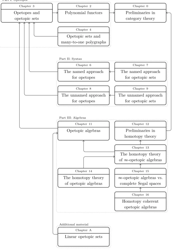
Figure 1: Chapter dependency graph

Chapter 0 Preliminaries in category theory Chapter 2 Polynomial functors Chapter 3 Opetopes and opetopic sets Chapter 4

Opetopic sets and many-to-one polygraphs

Chapter 6

The named approach for opetopes

Chapter 7

The named approach for opetopic sets

Chapter 8

The unnamed approach for opetopes

Chapter 9

The unnamed approach for opetopic sets

Chapter 11 Opetopic algebras Chapter 12 Preliminaries in homotopy theory Chapter 13

The homotopy theory of ∞-opetopic algebras

Chapter 14

The homotopy theory of opetopic algebras

Chapter 15

∞-opetopic algebras vs. complete Segal spaces

Chapter 16

Homotopy coherent opetopic algebras

Chapter A

Linear opetopic sets

Part I: Opetopes

Part II: Syntax

Part III: Algebras

(20)

Acknowledgments

F

irst and foremost, I would like to thank my PhD advisors, Pierre-Louis Curien andSamuel Mimram, for their kind attention and guidance. I greatly benefited from their ideas and experience, not only in mathematics and theoretical computer science, but also in the world of scientific research as a whole. I also enjoyed the freedom they gave me in my research, while still remaining readily available.

I would like to thank Nicola Gambino and Marek Zawadowski for kindly accepting to review my thesis. I am also grateful to Denis-Charles Cisinski, Eugenia Cheng, Geoffroy Horel, and François Métayer for accepting to take part in my defense jury. I am very honored to present my work to them.

I would not be where I am today without the love and unyielding support of my family. I am extremely grateful to my wonderful wife Amanda, my caring parents Christine and Tuyen, and my younger sister Delphine.

And now, the regulatory roll call of my fellow colleagues. I would like to thank Chai-tanya for collaborating with me on a few articles, always having time to answer technical questions, and giving me very valuable insights and pointers into the Big Picture. I would like to thank Zeinab for caring about the PhD students well-being with cakes and sofas; I will miss getting coffee and ruling today’s math problem as uninterestingTM. Alen for being a quiet neighbor, avid French learner, and not taking all of Pierre-Louis’s time. Théo for always having something interesting to discuss about during lunch break. Axel and Léonard for being reliable category theory references. Rémi for his continuous-but-nowhere-differentiable enthusiasm. Léo for being considerate of my hearing by speaking quietly. Daniel for bringing Puiseux series to my attention. Nicolas for explaining what NP completeness is with his hairstyle. Victor for setting up the most amazing IRIF Cake web-site [Lan18]. I would also like to thank Jules, Antoine, Farzad, Simon, the other Simon, Thibaut, Baptiste, Antonin, the 3rd _{floor coffee machine, Abhishek, Kostia, Tommaso,} Bob, Bob 2, and obviously everyone else.

Apparently I can write what I want here. I would like to thank some of the previous occupants of oﬀice 3033 for cleaning behind them like any reasonable adult would. I would like to thank my LA_{TEX compiler for its clear and easy to understand error messages. I} extend my gratitude and admiration to Dr. Alexis Lemaire and his brilliant thesis [Lem10] for enlightening me about the real value of a PhD. I would like to thank Vinci for caring about my safety in the unlikely event of a fire.

Finally, I would like to apologize for absolutely nothing.

Funding. This thesis has received funding from the European Union’s Horizon 2020

re-search and innovation program under the Marie Sklodowska–Curie grant agreement No. 665850. I am also very grateful for the financial support provided by the πr2 _team.

(21)

(22)

Chapter Zero

Preliminaries in category theory

I

n this first chapter, we recall some notions and results in category theory, whichshall be used implicitly most of the time. We assume that the reader is familiar with elementary category theory. Good references on the matter can be found in [ML98] [Awo10] [Bor94a] [Rie17].

0.1 GENERALITIES

Notation 0.1.1. We write Cat for the (large) category of small categories, i.e. that in

which the class of objects and morphisms is a set, and _{Cat for the large (in some} uni-verse) category of (smaller) categories. Let_{C and D be categories (of any size), and write} DC_{∶= Cat(C, D) for the category of functors from C to D, and natural transformations.}

Notation 0.1.2. For n∈ N, let [n] be the linear order on n+1 elements, seen as a category:

[n] ∶= (0 Ð→ 1 Ð→ 2 Ð→ ⋯ Ð→ n) .

In particular, if _{C ∈ Cat, then C}[1] is the arrow category of _{C, whose objects are the} morphisms ofC, and morphisms are commutative squares.

Definition 0.1.3 (Comma category). Consider two functors F ∶ A Ð→ C and G ∶ B Ð→ C. The comma category F_{/G (also denoted by (F ↓ G) in the literature) is defined as the} pullback F/G C[1] A × B C × C, ⌟ ∂ F×G

where ∂ maps a morphism m∶ c Ð→ d to the tuple (c, d). If A = C and F is the identity functor, then we write F_{/G = C/G. If F is constant at an object c ∈ C, then we write}

F/G = c/G. In particular, if F = id_C and G is constant at c, then F_{/G = C/c is the} usual slice category. Those notations transpose to the case where G is an identity or F is constant.

Definition 0.1.4 (3-for-2). Let_{C be a category. We say that a class of morphisms K ⊆ C}[1] has the 3-for-2 property if for any pair _{(f, g) of composable morphisms, if two among f,}

g, and gf are in K, then so is the third.

Definition 0.1.5 (Cell complex). Let K be a class of morphisms of C. A relative K-cell

complex is a transfinite composition of pushouts of morphisms of K. We write Cell_K for 1

(23)

the class of relative K-cell complexes. If_{C has an initial object ∅, then a K-cell complex is} an object X _{∈ C such that the initial map ∅ Ð→ X is a relative cell complex.}

Definition 0.1.6 (Localization). LetC be a category, and K ⊆ C[1]be a class of morphisms of_{C. The localization, if it exists, is a category K}−1_{C equipped with a functor γ ∶ C Ð→ K}−1_C mapping all morphisms of K to isomorphisms, and which is initial for this property, i.e. if F ∶ C Ð→ D also maps morphisms of K to isomorphisms, then there exists a unique ¯F

making the following triangle commute:

C D K−1C. F γ ¯ F 0.2 LIFTING PROPERTIES

Definition 0.2.1 (Lifting property). LetC be a category, and l, r ∈ C[1]. We say that l has the left lifting property against r (equivalently, r has the right lifting property against l), written l_{⋔ r, if for any solid commutative square as follows, there exists a (non necessarily} unique) dashed arrow making the two triangles commute:

⋅ ⋅

l r (0.2.2)

Notation 0.2.3. Let c∈ C and f ∈ C[1]. If C has a terminal object 1, then we write f ⋔ c for

f ⋔ (c Ð→ 1). Dually, if C has an initial object 0, we write c ⋔ f for (0 Ð→ c) ⋔ f.

Let L and R be two classes of morphisms of_{C. We write L ⋔ R if for all l ∈ L and r ∈ R} we have l⋔ r. The class of all morphisms r (resp. l) such that L ⋔ r (resp. l ⋔ R) is denoted L⋔ (resp. ⋔R). We also write L⋔ (resp. ⋔R) for the category spanned by objects c∈ C such that L_{⋔ c (resp. c ⋔ R) and morphisms f such that L ⋔ f (resp. f ⋔ R), and although this} is ambiguous, the context shall always make it clear.

Definition 0.2.4 (Saturated class). We say that the class of morphisms K is saturated if K=⋔(K⋔). The saturation of K is the smallest saturated class containing K, i.e. ⋔(K⋔). Lemma 0.2.5. If K⊆ C[1] is a class of morphisms, then(⋔(K⋔))⋔ = K⋔ and⋔((⋔K)⋔) = ⋔K. Definition 0.2.6 (Orthogonality). We say that l is left orthogonal to r (equivalently, r is right orthogonal to l), written l _{⊥ r, if for any solid commutative square as in} equa-tion (0.2.2), there exists a unique dashed arrow making the two triangles commute. The relation_{⊥ is also known as the unique lifting property. The notations for ⋔ presented above,} e.g. L⋔, still make sense when_{⋔ is replaced by ⊥.}

Lemma 0.2.7. If L∶ C Ð→_{←Ð D ∶ R is an adjunction, f ∈ C}[1], and g∈ D[1], then Lf ⋔ g if and only if f _{⋔ Rg. Likewise, Lf ⊥ g if and only if f ⊥ Rg.}

Definition 0.2.8 (Local isomorphism). Let K be a class of morphisms of_{C. A morphism}

f ∈ C[1] is a K-local isomorphism if for all c∈ C such that K ⊥ c, we have f ⊥ c. Note that the class of K-local isomorphism is not ⊥_(K⊥_).

(24)

0.3 PRESHEAVES

Notation 0.3.1. LetC be a small category, and let Psh(C) ∶= SetCop be the category of ( Set-valued) presheaves over _{C. The Yoneda embedding will be denoted by y}_C _{∶ C Ð→ Psh(C),} or just y is the context is clear. Recall that, as the name suggests, it is an embedding, and that it exhibitsPsh(C) as the free cocompletion of C. As such, if c ∈ C, we sometimes write c instead of yc.

Definition 0.3.2 (Cell counting function). If X _{∈ Psh(C) is a presheaf over a small} category _{C, let #X be the cardinality of the sum ∑}_c_∈CXc. As a shorthand, we write #c∶= #yc, for c ∈ C.

Definition 0.3.3 (Shape). Let X∈ Psh(C). An element x ∈ Xc for some c∈ C is called a

cell of X of shape c, which we write x♮_{= c.}

Definition 0.3.4 (Category of elements). For f _{∶ c Ð→ d a morphism in C, we write}

f ∶ XdÐ→ Xc instead of Xf or f∗. The category of elements C/X (also denoted by ∫_CX) of X has objects all the cells of X, and a morphism f ∶ x Ð→ y in C/X is a morphism

f∶ y♮Ð→ x♮ in_{C such that f(x) = y. Note that for all c ∈ C, the category of elements of yc} is simply the slice_C/c.

Remark 0.3.5. In the literature, _{C/X is rather defined as the comma category y}_C_{/X (see}

definition 0.1.3), i.e. as the category of pairs (x, c) where c ∈ C and x ∈ Xc. Here, we consider that the shape c of x is an intrinsic data that can be retrieved using₍₋₎♮. Proposition 0.3.6 ([Lei04, proposition 1.1.7]). There is an equivalence of categories

Ψ∶ Psh(C)/XÐ→ Psh(C/X)≃

where if p∶ Y Ð→ X is a presheaf over X, and x ∈ C/X, then ΨYx= p−1(x).

Definition 0.3.7 (The category of simplices). Let ∆, the category of simplices, be the full subcategory of Cat spanned by categories of the form [n], where n ranges over N. It admits a well-known presentation [Jar06, section 1.1] [Hov99, section 3.1], where the generators, respectively called coface and codegeneracy, are denoted by di_{∶ [n − 1] Ð→ [n]} and si _{∶ [n + 1] Ð→ [n], where 0 ≤ i ≤ n. Specifically, d}i _{is the unique increasing map that} does not have i_{∈ [n + 1] in its image, while s}i _{has it twice.}

Definition 0.3.8 (Lifting problem). Let _{C be a small category, c ∈ C, x ∶ X ↪}_{Ð→ c be a} subpresheaf of the representable c, and Y ∈ Psh(C). An x-lifting problem of Y is simply a morphism f _{∶ X Ð→ Y . It is solved is there exists a ¯}f ∶ c Ð→ Y (called a solution) extending f : X Y c f x ¯ f

(25)

Definition 0.3.9. Let_{C be a small category, and D be a category with coproducts. There} is a functor _{− ⊠ − ∶ Psh(C) × D Ð→ D}Cop, called the box product induced by the coproducts

of D, where for X ∈ Psh(C), c ∈ C, and d ∈ D,

(X ⊠ d)c∶= ∑ Xc

d.

Note that if _{C = [0] is the discrete category with one object, then this construction gives} a functor Set × D Ð→ D, where for X ∈ Set and d ∈ D, we have X ⊠ d = ∑_Xd.

Dually, if_{D has all products, then there is a natural exponentiation functor Psh(C)}op × D Ð→ DCop

, where for X_{∶ C Ð→ Set, c ∈ C, and d ∈ D,} (dX₎

c ∶= ∏ Xc

d.

It_{C = [0], then this construction gives rise to a functor Set}op_{×D Ð→ D, where for X ∈ Set} and d_{∈ D we have d}X _{= ∏}

Xd.

Example 0.3.10 (Simplicial set). A presheaf X _{∈ Psh(∆) is called a simplicial set. We} write Xn instead of X_[n], and ∆[n] instead of y[n].

Let ∂∆_{[n], the boundary of [n], be the maximal subpresheaf of ∆[n] not containing} id_[n]∈ ∆[n]n. It is the smallest subpresheaf of ∆[n] containing the cofaces

([n − 1] di

Ð→ [n]) ∈ ∆[n]n−1 for 0_{≤ i ≤ n. We also say that it is spanned by the d}i_{’s. Write b}

n∶ ∂∆[n] Ð→ ∆[n] for the natural boundary inclusion, and B for the set of all boundary inclusions.

For 0_{≤ k ≤ n, the k-horn Λ}k_{[n] is the maximal subpresheaf of ∂∆[n] not containing}

dk. Let hk

n∶ Λk[n] Ð→ ∆[n] be the natural horn inclusion, and denote by H the set of all horn inclusions. If 0 < k < n, the horn is called inner, and let Hinner be the set of inner horn inclusions.

Definition 0.3.11 (Anodyne extension). Let An_∶=⋔_(H⋔_{) be the saturation of the set of} horn inclusions. An element of An is called an anodyne extension. Similarly, let An_inner, the class of inner anodyne extensions, be the saturation of Hinner.

Definition 0.3.12. A simplicial set X ∈ Psh(∆) is a quasi-category [BV73] (or inner Kan

complex) if Hinner⋔ X, i.e. all inner horn lifting problems of X are solved.

0.4 KAN EXTENSIONS

Theorem 0.4.1. (1) [ML98, proposition IX.5.1] If D is complete, then every functor F ∶ Cop× C Ð→ D has an end. Dually, if D is cocomplete, then every such F has a coend.

(2) [Lor19, theorem 1.4.1] Let F, G∶ C Ð→ D be two functors, where D has all limits. We have

DC_{(F, G) ≅ ∫}

(26)

(3) [Lor19, proposition 2.2.1] (density formula) Let _{C be a small category, and X ∈}

Psh(C). We have

X ≅ ∫

c∈C

Xc⊠ yc

where − ⊠ − ∶ Set × Psh(C) Ð→ Psh(C) is defined in definition 0.3.9.

Notation 0.4.2. LetC be a small category, X ∶ Cop _{Ð→ Set, and Y ∶ C Ð→ Set. The coend} ∫cXc× Y c admits the following simple description as a quotient in Set:

∫ c∈CXc× Y c = ∑c∈CXc× Y c

∼

where for f _{∶ c Ð→ d, x ∈ Xd, y ∈ Y c, we have an identification} (x, Y f(y)) ∼ (Xf(x), y) .

The class of a pair(u, v) ∈ Xc×Y c will be denoted by u⊗v. Abusing notations a little bit, the equivalence relation_{∼ above then translates to the very familiar identity x ⊗ f(y) =}

f(x) ⊗ y.

Definition 0.4.3 (Left Kan extensions [ML98, section X.5]). Consider a diagram of ca-tegories

C D

E F K

whereD is cocomplete. The (pointwise) left Kan extension LanKF of F along K is the functor_{E Ð→ D given by}

LanKF(e) ∶= colim

Ka→eF a = ∫ a∈C

E(Ka, e) ⊠ F a, (0.4.4) where_{⊠ is defined in definition 0.3.9. Using notation 0.4.2, Lan}_KF(e) is the set of tensors f⊗ x, where f ∶ Ka Ð→ e and x ∈ F a, subject to the identity

(g ⋅ Kϕ) ⊗ y = g ⊗ (Kϕ)(y),

where g ∶ Kb Ð→ e, y ∈ F a, and ϕ ∶ a Ð→ b. The left Kan extension of F comes with a natural transformation α_{∶ F Ð→ (Lan}_KF) ⋅ K which is initial among all natural

trans-formations of the form F _{Ð→ G ⋅ K, where G ∶ E Ð→ D. Dually, if D is complete, the}

(pointwise) right Kan extension RanKF of F along K is the functor E Ð→ D given by RanKF(e) ∶= lim

e→KaF a = ∫a∈CF a

E(e,Ka)_, _(0.4.5) where the exponentiation is defined in definition 0.3.9. The right Kan extension of F comes with a natural transformation β_{∶ (Ran}_KF)⋅K Ð→ F which is terminal among all natural

transformations of the form GKÐ→ F , where G ∶ E Ð→ D.

Proposition 0.4.6 ([ML98, corollary X.3]). Consider a diagram of categories

C D

E F K

(27)

where K is fully faithful. If _{D is cocomplete, then the universal natural transformation} α ∶ F Ð→ (LanKF) ⋅ K is a natural isomorphism. Dually, if D is complete, then the

universal natural transformation β ∶ (RanKF) ⋅ K Ð→ F is a natural isomorphism.

Remark 0.4.7. Throughout this thesis, we shall mainly consider left Kan extensions along

the Yoneda embedding. Given

C D

Psh(C) F y_C

and X _{∈ Psh(C), the coend of equation (0.4.4) becomes} Lany_CF(X) = ∫

c∈C

Xc⊠ F c. (0.4.8)

Since y_Cis dense, by proposition 0.4.6, there is an isomorphism F c_{≅ Lan}_y_CF(y_Cc) natural

in c∈ C.

Definition 0.4.9 (Nerve of a functor). A functor F ∶ C Ð→ D induces a nerve NF ∶ D Ð→ Psh(C), mapping d ∈ D to the presheaf D(F −, d) ∈ Psh(C).

Definition 0.4.10 (Dense functor [ML98, section X.6]). A functor G∶ A Ð→ B is dense if for all b_{∈ B we have}

b ≅ colim

Ga→bGa. Equivalently, G is dense if LanGG≅ id_B.

Proposition 0.4.11. (1) The nerve NF is fully faithful if and only if F is dense.

(2) If _{D is cocomplete, we have an adjunction Lan}_yF ∶ Psh(C) Ð→_{←Ð D ∶ N}F.

Notation 0.4.12 (The classical setting). Let F _{∶ A Ð→ B be a functor. Using Kan}

exten-sions, we obtain two adjunctions

F!∶ Psh(A) Ð→←Ð Psh(B) ∶ F∗, F∗∶ Psh(B) Ð→←Ð Psh(A) ∶ F∗,

where F_! (resp. F_∗) is the left (resp. the right) Kan extension of _A _{Ð→ B}F _{Ð→ Psh(B)}yB along the Yoneda embedding y_A, and F∗= Ny_B⋅F is the precomposition by F .

Unfolding definitions, for X_{∈ Psh(A) and b ∈ B, we have}

F!Xb = ∫ a∈A

Xa× B(b, F a), (0.4.13)

and for Y _{∈ Psh(B) and a ∈ A, we have F}∗Ya= YF a. Therefore,

F!F∗Yb = ∫ a∈A

YF a× B(b, F a)

and the counit ε_Y _{∶ F}_!F∗Y Ð→ Y of the adjunction F!⊣ F∗ simply maps a tensor y⊗ f to

f(y), where y ∈ YF a and f∶ b Ð→ F a.

Lemma 0.4.14 ([SGA72, exposé I, proposition 5.6]). If any among F , F!, and F∗ is fully

(28)

0.5 LOCALLY PRESENTABLE CATEGORIES definition

Definition 0.5.1 (Filtered category). For κ a regular cardinal, a small category _{J is}

κ-filtered if every diagram of less than κ morphisms has a cocone. We say thatJ is filtered

if it is _ℵ0-filtered. A κ-filtered colimit is a colimit whose domain category is a κ-filtered category. A functor is finitary if it preserves filtered colimits.

Definition 0.5.2 (Presentable object [AR94, definition 1.13]). Let κ be a regular cardinal. An object c ∈ C is κ-presentable if C(c, −) preserves κ-filtered colimits. Equivalently, if

F ∶ J Ð→ C is a functor, where J is κ-filtered, then a morphism c Ð→ colim F factors

essentially uniquely through a F j, for some j _{∈ J. We say that c is presentable if it is}

κ-presentable, for some regular cardinal κ, and finitely presentable if it isℵ0-presentable. Example 0.5.3. InSet, the finitely presentable sets are exactly the finite sets. Indeed, let X be a finite set, F _{∶ J Ð→ Set be a filtered diagram, and take a map f ∶ X Ð→ colim F .} For each x _{∈ X, there exists a j}_x _{∈ J such that f(x) ∈ F j}_x. The discrete subcategory of J spanned by the jx’s is finite (since X is finite), thus has a cocone, say leading to an object j _{∈ J. Then f factors through F j. More generally, κ-presentable sets are those} whose cardinality is less than κ.

Definition 0.5.4 (Locally presentable category [AR94, definition 1.17]). Let _{C be a} ca-tegory. We say thatC is locally κ-presentable if it has all colimits, and if there exists a set of κ-presentable objects that generate_{C under κ-filtered colimits. It is locally presentable} if it is locally κ-presentable, for some regular cardinal κ, and finitely presentable if it is ℵ0-presentable. In the latter case, we writeCﬁnfor the full subcategory spanned by finitely presentable objects.

Example 0.5.5. (1) In _{Set, a set X is the union of its finite subsets, i.e. the colimit} of the canonical diagram _Set_fin_{/X. Since finite unions of finite sets are still finite,} this diagram is filtered. Thus the category Set is locally finitely presentable. The set of generating finitely presentable object can be taken to be any skeleton_Set_fin. (2) More generally, the category_{Psh(C) of presheaves over a small category C is locally} finitely presentable, and the finitely presentable objects are the finite colimits of representable presheaves. Note that a finitely presentable presheaf X _{∈ Psh(C)}_fin need not be finite in the sense that #X < ℵ0. For instance, no nonempty simplicial set has finitely many cells. However, if _{C is locally finite (i.e. all its slices C/c have} finitely many morphisms), then _Psh(C)_fin is exactly the category spanned by the presheaves with finitely many cells.

the gabriel–ulmer duality

Theorem 0.5.6 (Gabriel–Ulmer duality [GU71] [LP09, theorem 8]). Let _{Lex be the}

2-category of finitely complete small categories and finitely continuous functors, and _Lfp be the 2-category of locally finitely presentable categories and finitary right adjoints. Then the functor _{Lex(−, Set) ∶ Lex}op _{Ð→ Lfp is an equivalence of 2-categories. Consider the}

(29)

functor T _{∶ Lfp Ð→ Lex, that maps a locally finitely presentable category C to a skeleton} of _Cop_ﬁn. Then T is an inverse to _{Lex(−, Set) up to natural equivalence.}

Corollary 0.5.7 ([LP09, theorem 10]). If _{C a finitely locally presentable category, then} C ≃ Lex(Cop

ﬁn,Set).

the representation theorem

Definition 0.5.8 (Orthogonality class [AR94, definitions 1.32 and 1.35]). Let _{C be a} category, and κ be a regular cardinal. A subcategory _{D is a κ-orthogonality class if there} exists a class K of morphisms ofC whose domains and codomains are κ-presentable, such that _{D is the full subcategory spanned by those objects c ∈ C satisfying K ⊥ c. We say} that D is a small κ-orthogonality class if K is a set; it is an orthogonality class if it is a

λ-orthogonality class for some regular cardinal λ.

Example 0.5.9. Let n_{∈ N. The spine S[n] ⊆ ∆[n] is the colimit of the following diagram} in_Psh(∆):

∆[1] ∆[1] ∆[1] ⋯ ∆[1] ∆[1]

∆[0] ∆[0] ∆[0] ∆[0],

d1 d0 d1 d0 d1 d0 d1

where there are n instances of ∆_{[1]. In other words, it is a chain of n copies of ∆[1] glued} end to end. Let S_{∶= {S[n] ↪}_{Ð→ ∆[n] ∣ n ∈ N} be the set of spine inclusions. A simplicial} set X ∈ Psh(∆) such that S ⊥ X is said to satisfy the Segal condition. It is well-known that nerves of categories are exactly those simplicial sets that satisfy the Segal condition [Seg68]. Therefore, _{Cat is equivalent to the orthogonality class of Psh(∆) induced by S.} Since domains and codomains of morphisms of S are finitely presentable, it is an ℵ0 -orthogonality class.

Proposition 0.5.10 ([GZ67, proposition 1.3]). Let F _{∶ C Ð→}_{←Ð D ∶ U be an adjunction. The}

following are equivalent:

(1) the counit ε∶ F U Ð→ id_D is a natural isomorphism; (2) the right adjoint U is fully faithful;

(3) for K_{∶= {f ∈ C}[1]_{∣ F f is an iso.} the class of maps that F maps to isomorphisms,} the canonical factorization ¯F ∶ K−1C Ð→ D is an equivalence of categories.

Theorem 0.5.11 ([GU71, theorem 8.5]). Let _{C be a small category, and D be a small}

κ-orthogonality class of Psh(C) induced by a set K of maps.

(1) The inclusion U ∶ D Ð→ Psh(C) preserves κ-filtered colimits and has a left adjoint1. (2) The class of K-local isomorphisms is the smallest class of morphisms that contains

K, satisfies 3-for-2, and is closed under colimits (inPsh(C)[1]). Further, if F is the left adjoint of U , then a morphism f ∈ Psh(C)[1] is a K-local isomorphism if and only if F f is an isomorphism.

1_{In [AR94, section 1.37], the left adjoint is called the orthogonal-reflection construction. Much in the}

spirit of Quillen’s small object argument [Hov99, theorem 2.1.14], it takes a presheaf X ∈ Psh(A) and iteratively adds and collapses cells, forming a sequence X = X(0) _{Ð→ X}(1) _{Ð→ ⋯ Ð→ X}(α)_{Ð→ ⋯ that}

(30)

Corollary 0.5.12. With_{C, D, and K as in theorem 0.5.11, and writing F ∶ Psh(C) Ð→ D}

for the left adjoint of U , the canonical factorization ¯F ∶ K−1Psh(C) Ð→ D is an equivalence of categories.

Proof. Follows from proposition 0.5.10 and theorem 0.5.11.

Definition 0.5.13 (Projective sketch [AR94, paragraph 1.49]). A projective sketch (also called a limit sketch) is the datum of a category _{S, a class of distinguished diagrams}

Di ∶ Ji Ð→ S, and to each such diagram, a choice of a cone γi ∶ ci Ð→ Di over it (where

ci∈ S is considered as a constand functor JiÐ→ S). A projective sketch is small if there is only a set of distinguished diagrams.

Let _{E be a category with all limits. A model of S in E is a functor M ∶ S Ð→ E that} maps each cone γi to a limit cone of M Di. A morphism of models is simply a natural transformation. If the category_{E is omitted, it is assumed to be Set.}

Example 0.5.14. Lawvere theories [Law04] [HP07, definition 2.2] are projective sketches, where the distinguished diagrams are finite and discrete, and where the cones are product cones (although not all such projective sketches are Lawvere theories).

Theorem 0.5.15 (Representation theorem [AR94, theorem 1.46, corollary 1.52]). LetC

be a category and κ be a regular cardinal. The following are equivalent: (1) _{C is locally κ-presentable;}

(2) C is equivalent to a κ-orthogonality class2 in Psh(A) for some small category A; (3) _{C is equivalent to an accessibly embedded full reflective subcategory of Psh(A) for}

some small category_{A, i.e. C is a full subcategory of Psh(A) closed under κ-filtered} colimits, the embedding C ↪Ð→ Psh(A) preserves κ-filtered colimits, and has a left adjoint;

(4) _{C is equivalent to a category of models over a small projective sketch whose} distin-guished diagrams have less than κ morphisms.

Proof (sketch). (1) Ô⇒ (3) Let Cκ be the full subcategory spanned by a chosen set of κ-presentable objects generating _{C under κ-filtered colimits. For i ∶ C}κ ↪Ð→ C the inclusion, the adjunction Lan_yi ∶ Psh(Cκ) Ð→←Ð C ∶ Ni satisfies the required properties.

(3) _{Ô⇒ (1) Up to equivalence, we have a reflective adjunction F ∶ Psh(A) Ð→}_{←Ð C ∶ U} whereA is a small category, and one can check that the set {F a ∣ a ∈ A} generates C by filtered colimits.

(2) _{Ô⇒ (3) This is theorem 0.5.11.}

(3) Ô⇒ (4) Let i ∶ C ↪Ð→ Psh(A) be the embedding, L be its left adjoint. Let K ⊆ Psh(A)[1] be the set of all morphisms f _{∶ X Ð→ a such that a ∈ A and Lf is an} isomorphism. For such an f , let Df be the forgetful functorA/X Ð→ Psh(A), and

γf be the obvious cocone from Df to a. Then Aop endowed with all the cones γf, where f ranges over K, forms a small projective sketch, and the associated category of models is equivalent to _C.

2_{In a locally presentable category, a κ-orthogonality class is necessarily a small orthogonality class.}

(31)

(4) _{Ô⇒ (2) Assume that C is the category of models of the small projective sketch} S, with distinguished diagrams Di ∶ JiÐ→ S and cones γi ∶ di Ð→ Di. InPsh(Sop), consider the canonical morphisms

¯

γi ∶ ydi Ð→ lim (Ji Di

Ð→ SÐ→ Psh(S))y

and let Γ be the set of all the ¯γi’s. Then domains and codomains of maps in Γ are

κ-small, andC is equivalent to the orthogonality class induced by Γ 3.

Example 0.5.16. Many classical algebraic structures, such as monoids, groups, abelian groups, rings, modules over a fixed ring, etc. are models of Lawvere theories, and in particular, models of projective sketches. Thus, those categories are all locally finitely presentable.

3_{Intuitively, we identify models of}_{S (those functors mapping the γ}

i’s to limit cones) to presheaves over

Sop_{that “see” the canonical morphisms d}

(32)

Part I

(33)

Opetopes: Syntactic and Algebraic Aspects

HAL Id: tel-02968939

https://hal.archives-ouvertes.fr/tel-02968939

Opetopes: Syntactic and Algebraic Aspects

Cédric Ho Thanh

To cite this version:

Opetopes

syntactic and algebraic aspects

Cédric Ho Thanh

Contents

Introduction

H

P

P

P

Acknowledgments

F

Preliminaries in category theory

I

Part I