Lossy Video compression using well known mathematical functions and a limited set of reference values

(1)

Colonel Ahmed Draia University of Adrar Faculty of Sciences and Technology

Department of Mathematics and Computer Science

A Thesis Presented to Fulfill the Partial Requirement for Master’s Degree

in Computer Science

Option: Networks and Intelligent Systems

Title:

Lossy Video compression using well known

mathematical functions and a limited set of

reference values

Prepared by

Miss. Leyla OULAD BENSAID

Supervised by

Dr. Mohammed OMARI

(2)

Nowadays the amount of digital video applications is rapidly increasing. The amount of raw video data is very large which makes storing, processing, and transmitting video sequences very complex tasks. Furthermore, while the demand for enhanced user experience is growing, the sizes of devices capable of performing video processing operations are getting smaller. This further increases the practical limitations encountered when handling these large amounts of data, and makes research on video compression systems and standards very important. For this reason, many compression techniques have been proposed; some of these have been effective in some areas and failed in others. In this thesis we propose a new lossy video compression technique using well known mathematical functions and a limited set of reference values. Our approach is based on finding a compressed value whose corresponding pair of the corresponding mathematical function and reference value, aiming to produce shorter expressions compared to the regular form. In addition, we integrated an approach that utilizes binary search algorithm in order to efficiently find a better compressed value with shorter reduced form that does not harm the original image quality. The preliminary results of our method show promising results compared to other peer techniques.

Keywords: Lossy video compression, video codec, mathematical function

(3)

Acknowledgements

First, I thank Allah the Almighty for giving me courage, strength and patience to complete this modest work.

I wish to express my profound gratitude to Dr. OMARI Mohammed, my

Respected supervisor, for his excellent guidance, caring, patience, I ask Allah to bless him.

My respect and gratitude to the jury members who gave me the honor of judging this work through their availability, observations and reports that have enabled me to

enhance my scientific contribution.

Thanks to all the teachers of our faculty of Sciences and Technology.

(4)

Dedicates

I would like to dedicate this work

To the spring that never stops giving… To my mother To the big heart... My dear father

To the people who paved our way of science and knowledge All our distinguished teachers

(5)

LIST OF FIGURES

Figure 1.1: Example of frame rate. ... 5

Figure 1.2: Still image from natural video scene ... 7

Figure 1.3: Spatial and temporal sampling of a video sequence ... 7

Figure 1.4: Image with 2 sampling grids ... 8

Figure 1.5: Image sampled at coarse resolution (black sampling grid) ... 10

Figure 1.6: Image sampled at slightly finer resolution (grey sampling grid) ... 10

Figure 1.7: Interlaced video sequence. ... 11

Figure 1.8: Top field ... 12

Figure 1.9: RGB space.(put a dot at the end of each figure caption) ... 14

Figure 1.10: Example, RGB Colour components: R, G and B ... 14

Figure 1.11: Example of U-V color plane ... 15

Figure 1.12: An image along with its Y′, U, and V components respectively ... 15

Figure 1.13: The YIQ color space. ... 16

Figure 1.14: An image along with its Y, I, and Q components. ... 17

Figure 1.15: Video frame sampled at range of resolutions ... 17

Figure 1.16: Encoder / Decoder ... 19

Figure 1.17: Relation between codec, data containers and compression algorithms. ... 19

Figure 1.18: Example of PSNR ... 22

Figure 2.1: Original image (left) and JPEG compressed picture (right). ... 28

Figure 2.2: Original image (left) and JPEG 2000 compressed picture (right). ... 29

Figure 2.3: A three-picture JPEG video sequence. ... 30

Figure 2.4: A three-picture MPEG video sequence. ... 31

Figure 2.5: The illustration above shows how a typical sequence with I-, B-, and P-frames . 35 Figure 2.6: An interface in a network camera of the Group of Video (GOV). ... 36

Figure 3.1: The three phases of the proposed method ... 42

Figure 3.2: Sine And Cosine function graph ... 43

Figure 3.3: Tangent function graph ... 43

Figure 3.4: Square root function graph ... 43

(9)

Figure 3.10: Compressing a video ... 52

Figure 3.11: Compressed video, original video and compression results. ... 53

Figure 3.12: Screenshot describing the characteristics of the machine... 54

Figure 3.13: Number of functions selected by Frame-1 Video1 ... 57

Figure 3.19: Comparison between Proposed method and other methods ... 65

(10)

LIST OF TABLES

Table 1.1: 100% RGB Color Bars ... 13

Table 1.2: Video frame format (Uncompressed bit rates) ... 18

Table 1.3: Typical storage capacities ... 18

Table 1.4: Image and Video Compression Standards ... 21

Table 1.5: Digital Video Containers and File Quick Chart Explanation ... 24

Table 3.1: The set of function used in the proposed method ... 45

Table 3.2: Description the components of the interface. ... 51

Table 3.3: Obtained results for video 1 ... 63

(11)

GLOSSARY

AVC Advanced Video Coding

Block Region of macroblock (8 × 8 or 4 × 4) for transform purposes

B picture (slice) Coded picture (slice) predicted using bidirectional motion compensation

CCITT Block Matching Algorithms

CIF Common International Format, a colour image format

chrominance Colour difference component

CODEC COder / DECoder pair

colour space Method of representing colour images

DCT Discrete Cosine Transform

DPCM Differential Pulse Code Modulation

GOP Group Of Pictures, a set of coded video images

IDCT Inverse Discrete Cosine Transform

HVS Human Visual System, the system by which humans perceive and interpret visual images

H.261 A video coding standard

HD High Definition

HDTV High Definition Television

Huffman coding Coding method to reduce redundancy

IEC International Electrotechnical Commission, a standards body Inter (coding) Coding of video frames using temporal prediction or compensation interlaced (video) Video data represented as a series of fields

intra (coding) Coding of video frames without temporal prediction

I picture (slice) Picture (or slice) coded without reference to any other frame ISO International Organization for Standardization, a standards body

ITU-T Telecommunications Union-Telecommunication standardization sector, a

standards body

JPEG Joint Photographic Experts Group, a committee of ISO (also an image

coding standard)

JPEG2000 An image coding standard

MPEG Motion Picture Experts Group , a committee of ISO/IEC

MPEG-1 A multimedia coding standard

MPEG-2 A multimedia coding standard

(12)

P-picture (slice) Coded picture (or slice) using motion-compensated prediction from one

PSNR Peak Signal to Noise Ratio, an objective quality measure

QCIF Quarter Common Intermediate Format

RGB colour space Red/Green/Blue colour space

VHS Video Home System

YCbCr Luminance, Blue chrominance, Red chrominance colour space

(13)

Recent advances in digital technologies have paved the way to the development of numerous real-time applications deemed too complex in the past. A vast array of those applications requires transmission and storage of digital videos such as digital TV, video streaming, multimedia communications, remote monitoring, videophones and video conferencing. Advances in digital video can be classified as one of the most influential modern technologies; this is due to the fast wide spread use of digital video applications into everyday life. Consequently, over the last three decades, high-quality digital video has been the goal of companies, researchers and standardization bodies

In today’s world, video compression is a very important tool to save the amount of space the video uses for its storage. Instead of sending each frame one after another, the differences in the frames can be stored and transmitted to reduce the size and also to save time. This is the actual idea behind the video compression technique. In recent days, as the video streaming has been the trending topic, compression of the video has become more significant and vital.

There are many compression techniques for compressing the video or image. One of the most common methods of video compression is the Discrete Cosine Transform method. In spite of several advanced video compression methods being used, the basic steps used for still image compression can also be used along with the inclusion of motion estimation and compensation.

In this thesis we present a new lossy video compression method, this method based on mathematical functions. Our approach is based on finding the closest compression value for each sub-frame and record the corresponding mathematical function and reference value are of order of magnitude shorter than the original Sub-frame.

Our method has been proposed in order to provide sufficient high compression ratios with good performance, in terms of quality

(14)

concepts such as different video formats, video standards, some popular video file format and containers, and brief review about video compression technique; the most known nowadays.

The second chapter presents the general scheme of the various video compression techniques and some of its characteristics and the difference between these techniques.

The third chapter presents a detailed description of our proposed method, and presents the implementation and the results obtained from each experiment.

Lastly, the thesis is closed with a general conclusion and some insights on

(15)

CHAPTER 1

(16)

1.1. Introduction

Video coding is the process of compressing and decompressing a digital video signal. This chapter examines the structure and characteristics of digital images and video signals and introduces concepts such as sampling formats and quality metrics that are helpful to an understanding of video coding.

It starts by briefly describing the overall process of a basic video coding scheme. Then digital video concepts related to block based video coding are explained. Finally an overview of compression type such us lossy and lossless compression.

1.2. History of video compression

Raw video consists of a sequence of frames or pictures, therefore the principles of video compression are primarily based on image compression. Since the early 1980s the field of image and video coding has seen considerable progress. Many video coding systems and standards have been developed through the years. The most popular standards have been published by the International Telecommunications Union-Telecommunication standardization sector (ITU-T) [3][9], or by the International Organization for Standardization (ISO) [4][10] in conjunction with the International Electrotechnical Commission (IEC) [5][11]. The more recent standards were the result of the collaboration between experts from the two standardisation bodies.

In 1984, a Differential Pulse Code Modulation (DPCM) based video coding standard (H.120) was developed by the International Telegraph and Telephone Consultativ Committee (CCITT, forerunner of the ITU-T). The standard worked on line-by-line basis and achieved a target rate of 2 Mbits/s with good spatial resolution but with very poor temporal quality. An improvement of this standard was submitted to the ITU-T in the late 1980s. The new technology was based on the Discrete Cosine Transform (DCT). In parallel to ITU-T's investigation the Joint Photographic Experts Group (JPEG) was also interested in compression of static images, based on DCT as well. Also in the late 1980s, several lossy compression methods began to be used.

(17)

Examples of this include: run-length encoding, with codewords determined by Huffman coding and lossy DCT, then Huffman or arithmetic coding.

The H.261 [6][12] standard was recommended in 1988. This standard is considered the first practical digital video coding standard as all subsequent standards are based on the H.261 design. It was the first standard in which 16×16 array of luma samples called MacroBlock (MB), and inter-picture prediction to reduce temporal redundancy emerged. Transform coding using an 8×8 (DCT) to reduce the spatial redundancy as used.

During the 1990s, the Motion Picture Experts Group (MPEG) was aiming to develop a video codec capable of compressing movies onto hard disks, such as CD-ROMs, with a performance comparable to that of Video Home System (VHS) quality. MPEG 4 accomplished this task by developing the MPEG-l [7][13] standard based on the H.261 ramework. In MPEG-1 the speed was traded for compression efficiency since it mainly targeted video storage applications. MPEG-l decoders/players were rapidly adapted to multimedia on computers especially with the release of operating systems or multimedia applications for PC and Mac platforms. In 1994 a new generation of MPEG, called MPEG-2 was developed and soon implemented in several applications. MPEG-2 [8][14]had great successes in the digital video industry specifically in digital television broadcasting and DVD-Video. A slightly improved version of MPEG-2, called MPEG-3, was to be used for coding of High Definition (HD) TV, but since MPEG-2 could itself achieve this, MPEG-.3 standards were folded into MPEG-2.

The need for better compression tools led to the development of two further standards.

MPEG-4 [9][15] visual and H.264 Advanced Video Coding (AVC) [10][16]( also called MPEG-4 part-10) . MPEG-4 visual was designed to provide a flexible visual communications using object-oriented processing. In contrast, the H.264 was aiming to exploit previous technology but in a more efficient, robust and practical way. Its main advantages in comparison to previous standards are the wide variety of applications in which it can be used and its versatile design. This standard has shown significant rate distortion improvements when compared to other standards for video

(18)

compression. The first version of the standard was released in 2003. The H.264 different profiles has a very broad application range that covers products developed by different companies and broadcast satellite TV in different countries.

1.3. Concepts and Definitions

In an analogue system a video camera produces an analogue signal of an image scanned from left to right and from top to bottom making up a frame [17]. The choice of number of scanned lines per picture is a trade-off between the bandwidth, flicker and resolution.

Any video consists of frames of a scene taken at various subsequent intervals in time. Each frame represents the distribution of light energy and wavelength over a finite size area and is expected to be seen by a human viewer [18]. Digital frames have a fixed number of rows and columns of digital values, called picture elements or pixels. These elements hold quantised values that represent the brightness of a given color at any specific point [19]. The number of bits per pixel is known as pixel depth or bits per pixel.

1.3.1. Frame rate

The number of frames displayed per second. The illusion of motion can be experienced at frame rates as low as 12 frames per second [20]. Standard-Definition television typically uses 24 frames per second, and HD videos can use up to 60 frames per second.

(19)

1.3.2. Frame dimensions

The width and height of the image expressed in the number of pixels. Some common formats include:

• CIF (Common International Format), defines a video sequence with a resolution of 352 × 288.

• QCIF (Quarter CIF), defines a video sequence with a resolution of 176 × 144.

1.3.3.

Bit Rate (BR)

Numbers of bits that are processed per unit time are known as bit rate in computing. But more specifically in digital multimedia, we can say that the number of bits used in per unit time to represent a video or audio is known as bit rate. Higher bit rate will give higher video quality e.g. a VCD (Video Compact Disk) with the bit rate 1 Mbit/s has lower quality than a DVD (Digital Versatile Disk) with bit rate of 5 Mbits/s. There are two different types of bit rate.

• Variable Bit Rate (VBR): In any video section, there are different kinds of scenes. They can vary from very simple i.e. clear sky, to very complex i.e. a tree with a lot of branches and leaves. Therefore the number of bits required for a scene varies according to the scene complexity. The best way is to save bits from simple scenes and use them for complex one and that’s how a variable bit rate decoder works. Although process for calculating bit rate is very complex.

• Constant/Fixed Bit Rate (CBR): For some applications, we need to transmit data on a constant bit rate. Mostly broadcast mediums like cable or satellite etc have the limitation of fixed bit rate. Compressors for constant bit rate are not as efficient as variable bit rate encoders are, but still there are very high quality encoders provided by MPEG-2 systems for CBR.

VBR is much more efficient for achieving good quality. It gives constant good quality as it can change bit rate for complex scenes. On other hand CBR gives us variable quality of a video, as it has same bit rate for each n every scene of a video.[6]

(20)

1.3.4. Natural video scenes

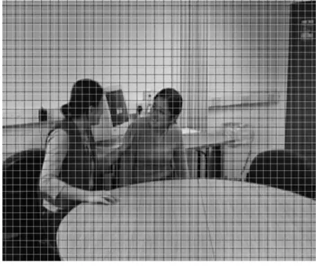
A typical ‘real world’ or ‘natural’ video scene is composed of multiple objects each with their own characteristic shape, depth, texture and illumination. The color and brightness of a natural video scene changes with varying degrees of smoothness throughout the scene (‘Continuous tone’). Characteristics of a typical natural video scene (Figure 1.1) that are relevant for video processing and compression include spatial characteristics (texture variation within scene, number and shape of objects, color, etc.) and temporal characteristics (object motion, changes in illumination, movement of the camera or viewpoint and so on). [1]

(21)

1.4. Capture

A natural visual scene is spatially and temporally continuous. Representing a visual scene in digital form involves sampling the real scene spatially (usually on a rectangular grid in the video image plane) and temporally (as a series of still frames or components of frames sampled at regular intervals in time) (Figure 1.2). Digital video is the representation of a sampled video scene in digital form. Each spatio-temporal sample (picture element or pixel) is represented as a number or set of numbers that describes the brightness (luminance) and colour of the sample. [1]

Figure 1.4: Image with 2 sampling grids.

To obtain a 2D sampled image, a camera focuses a 2D projection of the video scene onto a sensor, such as an array of Charge Coupled Devices (CCD array). In the case of color image capture, each colour component is separately filtered and projected onto a CCD array.

1.4.1. Spatial Sampling

The output of aCCDarray is an analogue video signal, a varying electrical signal that represents a video image. Sampling the signal at a point in time produces a sampled image or frame that has defined values at a set of sampling points. The most common format for a sampled image is a rectangle with the sampling points positioned

(22)

on a square or rectangular grid. Figure 1.4 shows a continuous-tone frame with two different sampling grids superimposed upon it.

Sampling occurs at each of the intersection points on the grid and the sampled image may be reconstructed by representing each sample as a square picture element (pixel). The visual quality of the image is influenced by the number of sampling points. Choosing a ‘coarse’ sampling grid (the black grid in Figure 1.4) produces a low-resolution sampled image (Figure 1.5) whilst increasing the number of sampling points slightly (the grey grid in Figure 1.4) increases the resolution of the sampled image (Figure 1.5).[1]

1.4.2. Temporal Sampling

A moving video image is captured by taking a rectangular ‘snapshot’ of the signal at periodic time intervals. Playing back the series of frames produces the appearance of motion. A higher temporal sampling rate (frame rate) gives apparently smoother motion in the video scene but requires more samples to be captured and stored. Frame rates below 10 frames per second are sometimes used for very low bit-rate video communications (because the amount of data is relatively small) but motion is clearly jerky and unnatural at this rate. Between 10 and 20 frames per second is more typical for low bit-rate video communications; the image is smoother but jerky motion may be visible in fast-moving parts of the sequence. Sampling at 25 or 30 complete frames per second is standard for television pictures (with interlacing to improve the appearance of motion, see below); 50 or 60 frames per second produces smooth apparent motion (at the expense of a very high data rate) [1].

(23)

Figure 1.5: Image sampled at coarse resolution (black sampling grid).

(24)

Figure 1.7: Interlaced video sequence.

1.4.3. Frames and Fields

A video signal may be sampled as a series of complete frames (progressive sampling) or as a sequence of interlaced fields (interlaced sampling). In an interlaced video sequence, half of the data in a frame (one field) is sampled at each temporal sampling interval. A field consists of either the odd-numbered or even-numbered lines within a complete video frame and an interlaced video sequence (Figure 1.7) contains a series of fields, each representing half of the information in a complete video frame (e.g. Figure1.8). The advantage of this sampling method is that it is possible to send twice as many fields per second as the number of frames in an equivalent progressive sequence with the same data rate, giving the appearance of smoother motion. For example, a PAL video sequence consists of 50 fields per second and, when played back, motion can appears smoother than in an equivalent progressive video sequence containing 25 frames per second.[1]

(25)

Figure 1.8: Top field.

1.5. Representation of colors:

For displaying a perfect color picture, three primary colors (red, green, blue) are basically needed. Because of this, every pixel contains minimum three different information channels. RGB and YUV are the generally used representation methods for colors. RGB includes the three primary colors along with the information about brightness. Generally the displays are monitored using this RGB representation. The color space is divided into chrominance (color) and luminance (brightness) in the YUV representation. Human beings are less sensitive to color than to brightness. Hence the chrominance information can be suppressed than the brightness information such that most of the quality is not lost. YUV data also helps in deriving the 3 basic colors (red, green, blue). In video compression, as the YUV representation produces better compression results, this representation is extensively used than the RGB representation. [2]

The three most popular color models are RGB (used in computer graphics); YIQ, YUV, or YCbCr (used in video systems); and CMYK (used in color printing). However, none of these color spaces are directly related to the intuitive notions of hue, saturation, and brightness. This resulted in the temporary pur- suit of other models,

(26)

such as HSI and HSV, to simplify programming, processing, and end- user manipulation.

All of the color spaces can be derived from the RGB information supplied by devices such as cameras and scanners.[21]

1.5.1. RGB coding

The RGB coding (Red, Green, and Blue), developed in 1931 by the International Lighting Commission (Commission Internationale de l'Eclairage, CIE) consist in representing the color space with three monochromatic rays, with the following colors:

• Red (with a wavelength of 700.0 nm), • Green (with a wavelength of 546.1 nm), • Blue (with a wavelength of 435.8 nm)

This color space corresponds to the way in which the colors are usually coded on a computer, or more precisely to the way in which the computer screen cathode tubes represent the colors. Thus, the RGB model proposes each color component to be coded on one byte, which corresponds to 256 intensities of red ), 256 intensities of green and 256 intensities of blue, thus, there are 16777216 theoretical possibilities of different colors, that is, many more than the human eye can distinguish (approximately 2 million). However, this value is only theoretical because it strongly depends on the display device being used1.Since RGB coding is based on three components with the same proposed value range, it is usually graphically represented by a cube of which each axis corresponds to a primary color: [4]

N om in al Ran ge W h ite Y ell ow C y an Gre en M age n ta Re d B lu e B lac k R 0 to 255 255 255 0 0 255 255 0 0 G 0 to 255 255 255 255 255 0 0 0 0 B 0 to 255 255 0 255 0 255 0 255 0

(27)

Figure 1.9: RGB space.

Figure 1.10: Example, RGB Colour components: R, G and B.

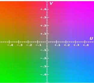
1.5.2. YUV Coding

YUV was originally used for PAL1 (European standard) analog video2. To convert from RGB to YUV spaces, the following equations can be used:

Y = 0.299 R + 0.587 G + 0.114 B U = 0.492 (B - Y)

V = 0.877 (R - Y)

Any errors in the resolution of the luminance (Y) are more important than the errors in the chrominance (U, V) values. The luminance information can be coded using higher bandwidth than the chrominance information.

(28)

Figure 1.11: Example of U-V color plane, Y′ value = 0.5, represented within RGB color gamut.

Figure 1.12: An image along with its Y′, U, and V components respectively.

1.5.3.

YIQ Color Space

The YIQ color space, is derived from the YUV color space and is optionally used by the NTSC composite color video standard. (The “I” stands for “in- phase” and the “Q” for “quadrature,” which is the modulation method used to transmit the color information.) The basic equations to convert between R´G´B´ and YIQ are:

Y = 0.299R´ + 0.587G´ + 0.114B´ I = 0.596R´ – 0.275G´ – 0.321B´ = Vcos 33° – Usin 33° = 0.736(R´ – Y) – 0.268(B´ – Y) Q= 0.212R´ – 0.523G´ + 0.311B´ = Vsin 33° + Ucos 33° = 0.478(R´ – Y) + 0.413(B´ – Y)

(29)

R´ = Y + 0.956I + 0.621Q G´ = Y – 0.272I – 0.647Q B´ = Y – 1.107I + 1.704Q

For digital R´G´B´ values with a range of 0– 255, Y has a range of 0–255, I has a range of 0 to ±152, and Q has a range of 0 to ±134. I and Q are obtained by rotating the U and V axes 33° These equations are usually scaled to simplify the implementation in an actual NTSC digital encoder or decoder.

Note that for digital data, 8-bit YIQ and R´G´B´ data should be saturated at the 0 and255 levels to avoid underflow and overflow wrap-around problems.

Figure 1.13: The YIQ color space at Y=0.5. Note that the I and Q chroma coordinates are scaled up to 1.0. See the formulae below in the article to get the right bounds.

(30)

1.6. Video formats

A variety of video standards are there which define the resolution and colors for display. For a PC, both the monitor and the video adapter determine the support for a graphics standard. The monitor must be capable of displaying the resolution and the colors defined by the standard whereas the video adapter needs to transmit the appropriate signals to the monitor. Some of the popular video standards along with their respective parameters are listed here in tabular forms.

Table 1 displays the uncompressed bit rates of some video formats. It can be clearly observed that even QCIF at 15 fps (i.e., relatively low quality video suitable for video telephony) requires 4.6 Mbps for storage or transmission. Table 2 shows typical capacities of popular storage media and transmission networks.[2]

Figure 1.15: Video frame sampled at range of resolutions [1].

Video format Colour Resolution

Intensity Resolution

Bits per second (uncompressed)

Frames per second

QCIF 88 x 72 176 x 144 4.6 Mbps 15

(31)

Media/Network Capacity

ADSL Typical 1-2 Mbps (downstream)

Ethernet LAN (10 Mbps) Maximum 10 Mbps / Typical 1-2 Mbps

V.90 MODEM 56 kbps downstream / 33 kbps upstream

ISDN-2 128 kbps

CD-ROM 640 Mbytes

DVD-5 4.7 Gbytes Table1.3: Typical storage capacities [2].

1.7. Video standards

Basically there are two families of standards:

1) ISO/IEC (International Standards Organization and International Electro- Technical Commission)

2) ITU (International Telecommunications Union)

 ISO/ IEC produced the MPEG standards which are the standard formats for video compression.

 ITU-T developed several recommendations for video coding such as H.261, H.263 starting from 1984 till it was approved in 1990. [2]

1.8. Video compression

Compression is the act or process of compacting data into a smaller number of bits. Video compression (video coding) is the process of converting digital video into a format suitable for transmission or storage, whilst typically reducing the number of bits. ‘Raw’ or uncompressed digital video typically requires a large bit rate, approximately 216Mbits for 1 second of uncompressed video [1]

(32)

Compression involves a complementary pair of systems, a compressor (encoder) and a decompressor (decoder). The encoder converts the source data into a compressed form occupying a reduced number of bits, prior to transmission or storage, and the decoder converts the compressed form back into a representation of the original video data. The encoder/decoder pair is often described as a CODEC (enCOder/DECoder) (Figure 1.16) [3]



Both combined form a codec and should not be confused with the terms data

container or compression algorithms.

1.8.1.

Lossy and lossless compression

Compression in general involves removing redundancies from the video sequence. It can be divided into two main types; lossless compression and lossy compression.[6]



Lossless compression allows a 100% recovery of the original data. It is usually

used for text or executable files, where a loss of information is a major damage. These compression algorithms often use statistical information to reduce redundancies. Huffman-Coding [23]and Run Length Encoding [24]are two

Codec

Compression algorithm

RealVideo Nero divX HDX4 MPEG-1 MPEG-2 MPEG-4 h.261 implements Packs coded files asf mpg avi

Figure 1.16: Encoder / Decoder[3].

Data Container

Quick Time M-JPEG

(33)



Using lossy compression does not allow an exact recovery of the original data. Nevertheless it can be used for data, which is not very sensitive to losses and which contains a lot of redundancies, such as images, video or sound. Lossy compression allows higher compression ratios than lossless compression. [5] Lossy compression schemes can achieve up to 95% higher compression rate than lossless compression schemes, this can be realised when comparing different commercial lossy and lossless encoders. Psychovisual redundancy can also be exploited because of the nature of Human Visual System (HVS) . The HVS does not perceive certain details in pictures. These pictures’ details can be discarded to reduce the size further without introducing perceivable errors in the reconstructed picture. [6]

1.8.2.

Why is video compression used?

A simple calculation shows that an uncompressed video produces an enormous amount of data: a resolution of 720x576 pixels (PAL), with a refresh rate of 25 fps and 8-bit colour depth, would require the following bandwidth:

720 x 576 x 25 x 8 + 2 x (360 x 576 x 25 x 8) = 1.66 Mb/s (luminance + chrominance) For High Definition Television (HDTV):

1920 x 1080 x 60 x 8 + 2 x (960 x 1080 x 60 x 8) = 1.99 Gb/s [5]

Even with powerful computer systems (storage, processor power, network bandwidth), such data amount cause extreme high computational demands for managing the data. Fortunately, digital video contains a great deal of redundancy. Thus it is suitable for compression, which can reduce these problems significantly. Especially lossy compression techniques deliver high compression ratios for video data. However, one must keep in mind that there is always a trade-off between data size (therefore computational time) and quality. The higher the compression ratio, the lower the size and the lower the quality. The encoding and decoding process itself also needs computational resources, which have to be taken into consideration. It makes no sense, for example for a real-time application with low bandwidth requirements, to

(34)

compress the video with a computational expensive algorithm which takes too long to encode and decode the data.[5]

1.8.3.

Image and Video Compression Standards

The following compression standards are the most known nowadays. Each of them is suited for specific applications. Top entry is the lowest and last row is the most recent standard. The MPEG standards are the most widely used ones, which will be explained in more details in the following sections. [5]

Standard Application Bit Rate

JPEG Still image compression Variable

H.261 Video conferencing over ISDN P x 64 kb/s

MPEG-1 Video on digital storage media (CD-ROM) 1.5Mb/s

MPEG-2 Digital Television 2-20 Mb/s

H.263 Video telephony over PSTN 33.6-? kb/s

MPEG-4 Object-based coding, synthetic content, Interactivity

Variable

JPEG-2000 Improved still image compression Variable

H.264/

MPEG-4 AVC

Improved video compression 10’s to 100’s kb/s

Table1.4: Image and Video Compression Standards.

1.9. Video Quality Measure

In order to evaluate the performance of video compression coding, it is necessary to define a measure to compare the original video and the video after compressed. Most video compression systems are designed to minimize the mean square error (MSE) between two video sequences Ψ1 and Ψ 2, which is defined as

(35)

Instead of the MSE, the peak-signal-to-noise ratio (PSNR) in decibel (dB) is more often used as a quality measure in video coding, which is defined as

It is worth noting that one should compute the MSE between corresponding frames, average the resulting MSE values over all frames, and finally convert the MSE value to PSNR. [7]

1.10. Explanation of File Formats

The different types of formats are technically referred to as “container formats." The differences between them lie in whether or not they compress the video and audio data they contain, and if so, how they go about compression.[25]

Each container has its own specific set of compatibility. For instance, some containers were developed by Microsoft with Windows users in mind. Likewise, Apple has its own proprietary containers for use on its Macintosh Operating Systems. Let’s list some of the common formats and their associations:

Option Format Description

AVI Video AVI stands for Audio Video Interleave. It is Microsoft’s video container format. .AVI files are good for Windows Media Player (WMP) and other online video players. The video retains quality, but they’re large files.

MOV Video A .Mov is a container file created by Apple to play QuickTime movies. .MOV and Mpeg 4 containers use the same MPEG-4 codecs and are usually interchangeable. MOV files do work on PCs. MOV files are large files, but they look great.

Figure 1.18:Example of PSNR.

(36)

MPEG4/MPEG Video MPEG stands for Motion Picture Experts Group. Many video cameras output footage in the MPEG format. YouTube converts uploaded videos to either Flash (FLV) or MPEG (MPG) formats. MPEG4 was created for the internet. It gives excellent quality and a small file up to 5x smaller than MOV files.

MP4 1080p or 1080i(HD)

Video Full 1920x1080 widescreen HD resolution perfect for HD-TV, Blu-Ray disks and high quality streaming. NBC and PBS broadcast in 1080i.

MP4 720p (HD) Video Standard 1280x720 HD resolution perfect for HD-TV, tablets, laptops and desktops. ABC, Fox and ESPN broadcast in 720p.

MP4 H.264 Video Codec for Blu-Ray disks. Widely used for YouTube, Vimeo, iTunes, Flash and also for HD-TV. Sony’s HD video cameras use AVCHD, which is H.264.

MP4 360p Video 640x360 resolution for standard definition (non HD) devices with a much smaller file size.

MP4 240p Video 640x360 resolution for standard definition (nonHD) devices with a smaller file size. This is always a Flash Video format. Use the MP4 360p rather than MP4 240p.

FLV (FLASH) Video Flash is the most common file used online and they play in the Adobe Flash Player that almost all computer users have downloaded on their computers for free. Apple is moving away from Flash so these files don’t work on iPhones and iPads. Many video sharing sites convert any video you upload to Flash files for sharing. The file sizes are of good quality and they’re small.

FLV 480p Video 640x480 pixel Flash Video Format best for movies on a tablet or similar large mobile device.

FLV 360p Video 640x360 pixel Flash Video Format great for blogs and most mobile devices.

FLV 240p Video 320x240 pixel Flash Video Format aimed at mobile devices and mobile websites.

NTSC 525 Video Non-HD, analog standard definition video used in the U.S. All TVs in the U.S. broadcast NTSC from 1941 until the conversion to HD. Aspect ratio 4:3. 30

(37)

WMV Video A WMV is a Windows Media Player format. They’re very compressed and don’t look great. They’re also PC nonMac) oriented. The files are so tiny that you can email video.

Table1.5: Digital Video Containers and File Quick Chart Explanation [8].

1.11. Conclusion

In this chapter we presented the structure and characteristics of digital images and video and introduce concepts such as sampling formats and quality metrics that are helpful to an understanding of video coding. We also touched on some concepts related to video codec such as frame rate, frame dimension and bit rate. In addition, we have deepened some basic concepts such different video format: QCIF, CIF, ITU-R601 and the two families of video standards. As we also talked briefly about video compression technique the most known nowadays and finally we mentioned some popular video file format and containers. .

(38)

CHAPTER 2

(39)

2.1. Introduction

Video compression reduces the quantity of data used to represent digital video content, making video files smaller with little perceptible loss in quality. In the last two decades, there are several video compression techniques developed. In this chapter we will discuss some of these video compression techniques and some of its characteristics and the difference between these techniques, we starts with an explanation of the basic concepts of video codec design and then explains how these various features have been integrated into international standards.

2.2. Video Compression Techniques

There are several video compression techniques developed in the last two decades. However the DCT compression and the wavelet compression are used much extensively. In video compression, the video is converted into individual frames and then compression techniques are applied on the images to compress the given file. The compressed images are decompressed and again a video could be created from those so that the compressed video is obtained. [2]

In the DCT method, the image is divided into small blocks and then the DCT is applied on each block. Applying DCT converts every pixel value into the frequency domain. DCT converts the pixel values into the frequency domain in such a way that the low frequencies are on the top-left and higher frequencies are on the bottom right. Then quantization is done so that the DCT coefficients become integers as they have been scaled by a scaling factor. By applying inverse discrete cosine transform (IDCT), original images can be reconstructed but not 100% similar to the actual ones. [2]

In wavelet compression, the compression techniques are applied on the image as a whole (i.e., image need not be divided into smaller blocks). The aim of this compression technique is to store the image data in as little space as possible. [2]

The standard formats for video compression such as the MPEG methods and the recommended methods such as H.261, H.263 are also used widely. MPEG standards

(40)

are again developed periodically to meet the required demands with the progress of time such as MPEG-1, MPEG-2, MPEG-4, MPEG-7, etc. [2]

2.3. Two basic standards: JPEG and MPEG

The two basic compression standards are JPEG and MPEG. In broad terms, JPEG is associated with still digital pictures, whilst MPEG is dedicated to digital video sequences. But the traditional JPEG (and JPEG 2000) image formats also come in flavors that are appropriate for digital video: Motion JPEG and Motion JPEG 2000 [27].

The group of MPEG standards that include the MPEG 1, MPEG-2, MPEG-4 and H.264 formats have some similarities, as well as some notable differences [27].

One thing they all have in common is that they are International Standards set by the ISO (International Organization for Standardization) and IEC (International Electrotechnical Commission) — with contributors from the US, Europe and Japan among others. They are also recommendations proposed by the ITU (International Telecommunication Union), which has further helped to establish them as the globally accepted de facto standards for digital still picture and video coding. Within ITU, the Video Coding Experts Group (VCEG) is the sub group that has developed for example the H.261 and H.263 recommendations for video-conferencing over telephone lines [27].

The foundation of the JPEG and MPEG standards was started in the mid-1980s when a group called the Joint Photographic Experts Group (JPEG) was formed. With a mission to develop a standard for color picture compression, the group’s first public contribution was the release of the first part of the JPEG standard, in 1991. Since then the JPEG group has continued to work on both the original JPEG standard and the JPEG 2000 standard [27].

In the late 1980s the Motion Picture Experts Group (MPEG) was formed with the purpose of deriving a standard for the coding of moving pictures and audio. It has

(41)

not concerned with the actual coding of multimedia, such as MPEG-7 and MPEG-21 [27].

2.4. The next step: H.264

At the end of the 1990s a new group was formed, the Joint Video Team (JVT), which consisted of both VCEG and MPEG. The purpose was to define a standard for the next generation of video coding. When this work was completed in May 2003, the result was simultaneously launched as a recommendation by ITU (“ITU-T Recommendation H.264 Advanced video coding for generic audiovisual services”) and as a standard by ISO/IEC (“ISO/IEC 14496-10 Advanced Video Coding”). Sometimes the term “MPEG-4 part 10” is used. This refers to the fact that ISO/IEC standard that is 4 actually consists of many parts, the current one being MPEG-4 part 2. The new standard developed by JVT was added to MPEG-MPEG-4 as a somewhat separate part, part 10, called “Advanced Video Coding”. This is also where the commonly used abbreviation AVC stems from.

2.5. An overview of video compression techniques

2.5.1. JPEG

JPEG is an acronym for Joint Photographic Experts Group. It is one of the compression techniques used for still image compression. It typically achieves a compression ratio of 10 upto acceptable loss of quality and as known already, there will be a tradeoff between the compression ratio and the quality. Generally most of the digital cameras save images in this format. For paintings on realities and for photography, JPEG is the best technique. JPEG is a type of lossy compression and it uses DCT approach to achieve the compression [2].

(42)

2.5.2. Motion JPEG

A digital video sequence can be represented as a series of JPEG pictures. The advantages are the same as with single still JPEG pictures – flexibility both in terms of quality and compression ratio. The main disadvantage of Motion JPEG (a.k.a. MJPEG) is that since it uses only a series of still pictures it makes no use of video compression techniques [26]. The result is a slightly lower compression ratio for video sequences compared to “real” video compression techniques [28].

2.5.3. JPEG 2000

This was developed after JPEG. Instead of the DCT approach used in the JPEG for compression, wavelet transformation is used in the JPEG 2000 and this technique achieves better compression ratios.

The main advantage of this technique over the JPEG is that the blockiness observed in the JPEG is removed and replaced by an overall fuzzy image, as shown in the following figure. [2]

(43)

Whether this fuzziness of JPEG 2000 is preferred compared to the “blockiness” of JPEG is a matter of personal preference. Regardless, JPEG 2000 never took off for surveillance applications and is still not widely supported in web browsers either. [27]

2.5.4. Motion JPEG 2000

As with JPEG and Motion JPEG, JPEG 2000 can also be used to represent a video sequence. The advantages are equal to JPEG 2000, i.e., a slightly better compression ratio compared to JPEG but at the price of complexity. The disadvantage reassembles that of Motion JPEG. Since it is a still picture compression technique it doesn’t take any advantages of the video sequence compression. This results in a lower compression ration compared to real video compression techniques. [28]

2.5.5. H.261/ H.263

These are not the international standards but the recommendations by the ITU. They can be considered as the simplified versions of the MPEG techniques. Since they were actually developed for low bandwidth i.e., for applications like video conferencing; they cannot provide the efficient usage of the bandwidth as some of the most advanced MPEG techniques are not included in these techniques. Hence it can be conclude that H.261 and H.263 are generally not used for video compression [2].

2.5.6. MPEG1

This was the basic compression standard developed by the ISO/IEC family in the year 1993. The idea is to store the video files in a format suited to CDROMs.

(44)

Using this standard, video is encoded at a data rate of less than 1.4 Mbps. This standard introduced the mp3 audio format which is the most popular today [2].

MPEG-1 video compression is based upon the same technique that is used in JPEG. In addition to that it also includes techniques for efficient coding of a video sequence [27].

Figure 2.3: A three-picture JPEG video sequence.

Consider the video sequence displayed in Figure 2.3. The picture to the left is the first picture in the sequence followed by the picture in the middle and then the picture to the right. When displayed, the video sequence shows a man running from right to left with a house that stands still [27].

In Motion JPEG/Motion JPEG 2000 each picture in the sequence is coded as a separate unique picture resulting in the same sequence as the original one.

In MPEG video only the new parts of the video sequence is included together with information of the moving parts. The video sequence of Figure 3 will then appear as in Figure 4. But this is only true during the transmission of the video sequence to limit the bandwidth consumption. When displayed it appears as the original video sequence again [27].

(45)

Figure 2.4: A three-picture MPEG video sequence.

MPEG-1 is focused on bit-streams of about 1.5 Mbps and originally for storage of digital video on CDs. The focus is on compression ratio rather than picture quality. It can be considered as traditional VCR quality but digital instead [28].

It is important to note that the MPEG-1 standard, as well as MPEG-2, MPEG-4 and H.264 that are described below, defines the syntax of an encoded video stream together with the method of decoding this bitstream. Thus, only the decoder is actually standardized. An MPEG encoder can be implemented in different way and a vendor may choose to implement only a subset of the syntax, providing it provides a bitstream that is compliant with the standard. This allows for optimization of the technology and for reducing complexity in implementations. However, it also means that there are no guarantees for quality – different vendors implement MPEG encoders that produce video streams that differ in quality [27].

2.5.7. MPEG-2

MPEG-2 is the "Generic Coding of Moving Pictures and Associated Audio." The MPEG-2 standard is targeted at TV transmission and other applications capable of 4 Mbps and higher data rates. MPEG-2 features very high picture

quality. MPEG-2 supports interlaced video formats, increased image quality, and other features aimed at HDTV[28].

MPEG-2 is a compatible extension of MPEG-1, meaning that an MPEG-2 decoder can also decode MPEG-1 streams.

(46)

MPEG-2 audio will supply up to five full bandwidth channels (left, right, center, and two surround channels), plus an additional low-frequency enhancement channel, or up to seven commentary channels. The MPEG-2 systems standard specifies how to combine multiple audio, video, and private-data streams into a single multiplexed stream and supports a wide range of broadcast, telecommunications, computing, and storage applications. MPEG-2, ISO/IEC 13818, also provides more advanced techniques to enhance the video quality at the same bit-rate. The expense is the need for far more complex equipment. Therefore these features are not suitable for use in real-time surveillance applications. As a note, DVD movies are compressed using the techniques of MPEG-2 [28].

2.5.8. MPEG-3

This was developed as an extension to MPEG-2 but later it was found that by making small adjustments to the MPEG-2, it performs the operations to be done by MPEG-3 i.e., to handle HDTV. Hence the research on MPEG-3 has not been done widely and now it has been stopped [2].

2.5.9. MPEG-4

The next generation of MPEG, MPEG-4, is based upon the same technique as MPEG-1 and MPEG-2. Once again, the new standard focused on new applications. The most important new features of MPEG-4, ISO/IEC 14496, concerning video compression are the support of even lower bandwidth consuming applications, e.g. mobile devices like cell phones, and on the other hand applications with extremely high quality and almost unlimited bandwidth. In general the MPEG-4 standard is a lot wider than the previous standards. It also allows for any frame rate, while MPEG-2 was locked to 25 frames per second in PAL and 30 frames per second in NTSC.

When “MPEG-4,” is mentioned in surveillance applications today it is usually MPEG-4 part 2 that is referred to. This is the “classic” MPEG-4 video streaming standard, a.k.a. MPEG-4 Visual.

Some network video streaming systems specify support for “MPEG-4 short header,” which is an H.263 video stream encapsulated with MPEG-4 video stream

(47)

specified in the 4 standard, which gives a lower quality level than both MPEG-2 and MPEG-4 at a given bit-rate. [MPEG-27].

2.5.10. H.264

H.264 is the result of a joint project between the ITUT’s Video coding Experts group and the ISO/IEC Moving Picture Experts Group (MPEG). ITU-T is the sector that coordinates Telecommunication standard on behalf of the International Telecommunication Union. ISO stands for International Organization for Standardization and IEC stands for International Electrotechnical Commission, which oversees standards for all electrical, electronic and related technologies [13]. H.264 is the name used by ITU-T, while ISO/IEC has named it MPEG-4 Part 10/AVC since it is presented as a new part in its MPEG-4 suite. The MPEG-4 suite includes, for example, MPEG-4 Part 2, which is a standard that has been used by IP-based video encoders and network cameras.

Designed to address several weaknesses in previous video compression standards, H.264 delivers on its goals of supporting:

1) Implementations that deliver an average bit rate reduction of 50%, given a fixed video quality compared with any other video standard.

2) Error robustness so that transmission errors over various networks are tolerated. 3) Low latency capabilities and better quality for higher latency.

4) Straightforward syntax specification that simplifies implementations.

5) Exact match decoding, which defines exactly how numerical calculations are to be made by an encoder and a decoder to avoid errors from accumulating.[28]

2.5.11. MPE G-7

This technique does not involve in the compression of any moving image or audio. This is often used in the video surveillance. Multimedia content description interface is done here. A meta-data for audio-video streams is generated by the MPEG-7. Though this model does not depend on the actual multimedia compression techniques, the MPEG-4 representation can also be suited to the MPEG-7 technique. Some of the applications of MPEG-7 are used in video analytics. [2]

(48)

2.5.12. MPEG-21

MPEG-21 is a standard that defines means of sharing digital rights, permissions, and restrictions for digital content. MPEG-21 is an XML-based standard, and is developed to counter illegitimate distribution of digital content. MPEG-21 is not particularly relevant for video surveillance situations.[27]

2.6. More on MPEG compression

MPEG-4 is a fairly complex and comprehensive standard that has some characteristics that are important to understand. They are outlined below[27].

2.6.1. Frame types

A video frame is compressed using different compression algorithms. For video frames, these different algorithms are called picture types or frame types. Basically there are three different frame types used in the different video compression algorithms. They are:

I-frames (don’t require other frames and is least compressible) P-frames (uses data from previous frame to decompress)

B-frames (uses data both from the previous frame and future frame to decompress)

 “I-frame means Intra frame in which every block is coded using raw pixel values, so it can always be decoded without additional information”.

 “P-frame is the name to define the forward Predicted pictures. The prediction is made from an earlier picture, mainly an I-frame, so that require less coding data (≈50% when compared to I-frame size)”.

 “B-frame is the term for bi-directionally predicted pictures. This kind of prediction method occupies less coding data than P-frames (≈25% when compared to I-frame size) because they can be predicted or interpolated from an earlier and/or later frame”[2].

(49)

Figure 2.5: The illustration above shows how a typical sequence with I-, B-, and P-frames may look. Note that a P-frame may only reference a preceding I- or P-frame, while a B-frame may

reference both preceding and succeeding I- and P frames.

The video decoder restores the video by decoding the bit stream frame by frame. Decoding must always start with an I-frame, which can be decoded independently, while P- and B-frames must be decoded

together with current reference image(s)[27].

2.6.2. Group of Pictures

A GOP specifies the order in which the frames are arranged. The group of successive pictures within a coded video stream is the GOP. Each encoded video stream contains successive GOPs. The visible frames are generated from the pictures contained within it [2].

One parameter that can be adjusted in MPEG-4 is the Group of Pictures (GOP) length and structure, also referred to as Group of Video (GOV) in some MPEG standards. It is normally repeated in a fixed pattern [27].

for example:

 GOV = 4, e.g. IPPP IPPP ...

 GOV = 15, e.g. IPPPPPPPPPPPPPP IPPPPPPPPPPPPPP ...  GOV = 8, e.g. IBPBPBPB IBPBPBPB ...

(50)

The appropriate GOP depends on the application. By decreasing the frequency of I-frames, the bit rate can be reduced. By removing the B-I-frames, latency can be reduced [27].

Figure 2.6: An interface in a network camera where the length of the Group of Video (GOV), i.e. the number of frames between two I-frames, can be adjusted to fit the application.

2.7. Other Compression Techniques

2.7.1. Intra frame coding and Inter frame coding

Inter frame coding refers to the compression done by comparing the data with the successive frames and just storing the differences between frames; whereas intra frame coding applies compression technique on every individual frame without any reference. This implies that the intra frame compression is effectively the image compression only. Some of the popular intra frame codecs are:

 MJPEG- JPEGs bunched together  Prores – Apple’s favorite

(51)

 Cinema DNG – Adobe’s baby for RAW image sequences Some of the popular inter frame codecs are:

 H.264  MPEG-2  MPEG-4  XD-CAM  XAVC  AVCHD

2.7.2. Run-length coding

In earlier days, this coding was used in fax machines to transmit the information. In this type of encoding all the pixel values are arranged in the form of an array and then checks for repetition of the same pixel values [27].

Suppose if the data is XXXXXXXYYYYYYYYYXXXXXXXYYYXX and run-length coding is applied on this data, that results in 7X9Y7X3Y2X i.e., the data is represented as 7X9Y7X3Y2X etc.

Hence using the run-length coding, the given data of 28 characters has been reduced to 10 characters and thus the compression is achieved.

To improve the compression ratios considerably, the original data should contain the less frequent runs and this will in turn cause the betterment in the compression ratios.

This compression comes under lossless compression and some other important lossless techniques are Huffman coding, Variable length-coding etc.

2.7.3. Variable Length Coding

This is one of the efficient lossless compression techniques. This coding technique encodes the data in such a way that more frequently occurring bits are encoded using short codes and the less frequently occurring bits are coded using more

(52)

number of bits. In this way, the number of bits used to transmit the data can be reduced after encoding the given data as explained above.

Huffman coding is an example of variable length-coding.

Winzip (one of the famous compression file) uses Huffman coding only.

2.7.4. Dynamic Pattern Substitution

This refers to the situation where no prior information of the frequently occurring symbols is available.

A look up table should be built while coding this type of bit stream [27].

2.7.5. Lempel-Ziv encoding

UNIX compress utility uses this type of coding technique and the objective is never to copy a sequence of bytes to the output stream which are previously seen by the encoder.

(53)

2.7.6. Progressive Scanning versus Interlaced Scanning

Progressive scanning is the technique in which all the fields in a frame are scanned one after the other. In interlaced scanning, all the fields are divided into odd and even fields and the scanning of all the odd fields (even fields) is done and then the scanning of the even fields (odd fields) occurs. The above figure clearly demonstrates the idea behind these two scanning techniques.

The progressive scanning has some drawbacks regarding the flickering and utilization of the bandwidth. Progressive scanning is also called the non-interlaced scanning. Progressive scanning is normally done in the televisions used in households [27].

2.8. Compression Constraints

2.8.1. Quality

While performing compression operations, the quality of the compressed video should be taken into account and the compressed video should not lose its quality beyond a certain acceptable level.

2.8.2. Complexity

While executing the different algorithms to obtain compression, the complexity of the algorithm is an important factor. It should not be too complex.

interlaced Progressive Scan

(54)

2.8.3. Delay

The execution time should be optimum while running a compression algorithm on a given video. While applying complex algorithms, it usually takes time to implement but the delay should not be very large.

2.8.4. Compression ratio

The ratio of the original file size to the compressed file size is called compression ratio. To obtain better compression ratios, the quality of the video has to be forfeited.

The above constraints for the compression are all very essential and according to the need of the user, there will be a tradeoff between these constraints. For example, both the better quality and high compression ratios cannot be achieved together. To achieve one of these, the other can be neglected.

2.9. Conclusion

In this chapter, we introduce the fundamental concepts of video compression and the characteristics of various video compression standards. Although the existed video compression standards can compress the video effectively, it still leaves room for improvement.

(55)