Chaos, entropy, and life-time in classical and quantum systems

HAL Id: tel-00189733

https://tel.archives-ouvertes.fr/tel-00189733

Submitted on 21 Nov 2007

HAL is a multi-disciplinary open access

archive for the deposit and dissemination of sci-entific research documents, whether they are pub-lished or not. The documents may come from teaching and research institutions in France or abroad, or from public or private research centers.

L’archive ouverte pluridisciplinaire HAL, est destinée au dépôt et à la diffusion de documents scientifiques de niveau recherche, publiés ou non, émanant des établissements d’enseignement et de recherche français ou étrangers, des laboratoires publics ou privés.

Chaos, entropy, and life-time in classical and quantum

systems

Seyed Majid Saberi Fathi

To cite this version:

Seyed Majid Saberi Fathi. Chaos, entropy, and life-time in classical and quantum systems. Mathe-matical Physics [math-ph]. Université Paris-Diderot - Paris VII, 2007. English. �tel-00189733�

THESE DE DOCTORAT

DE L’UNIVERSITE PARIS DIDEROT - PARIS 7

Sp´ecialit´e

Physique Th´eorique

pr´esent´ee par

Seyed Majid Saberi Fathi

Chaos, entropie et dur´

ee de vie dans les

syst`

emes classiques et quantiques

Soutenue le 19 juillet 2007 devant le jury compos´e de Messieurs:

Arno Bohm Pr´esident

Maurice Courbage Directeur de th`ese

Thomas Durt Examinateur

Tuong T. Truong Rapporteur

Table of Contents i

R´esum´e v

Abstract vii

Acknowledgements ix

Introduction (En Fran¸cais) 1

0.1 Premi`ere partie: Syst`emes chaotiques classiques . . . 1

0.2 Deuxi`eme partie: “Syst`emes instables quantiques” . . . 2

0.3 Pr´esentation . . . 5

Introduction 7 0.4 First part: Classical chaotic systems . . . 7

0.5 Second part: Unstable quantum systems . . . 8

0.6 Presentation . . . 10

I

Classical Chaotic Systems

13

1.1.1 Linearization . . . 16

1.2 Lyapounov Exponents . . . 17

1.2.1 The Lyapounov Exponent for a map in one dimension . . . 17

1.2.2 Lyapounov Characteristic Exponents . . . 18

1.2.3 Numerical computation of Lyapounov spectra . . . 20

1.3 Hard spheres model . . . 21

1.4 Lorentz gas . . . 24

1.5 H -theorem . . . . 24

1.6 Ergodic Theory . . . 26

1.6.1 Introduction . . . 27

1.6.2 Statement of Ergodic Theorem . . . 28

1.7 Coarse-graining . . . 29

1.8 Entropy . . . 32

1.8.1 Shannon entropy . . . 32

1.8.2 _{K − S entropy . . . .} 34

1.8.3 Entropy functional under coarse-graining . . . 34

2 Computation of entropy increase for Lorentz gas and hard disks 39 2.1 Introduction . . . 40

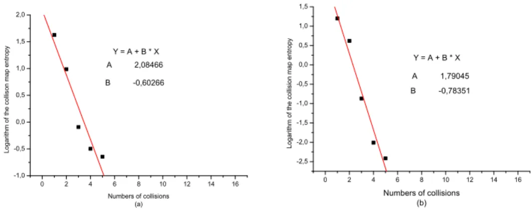
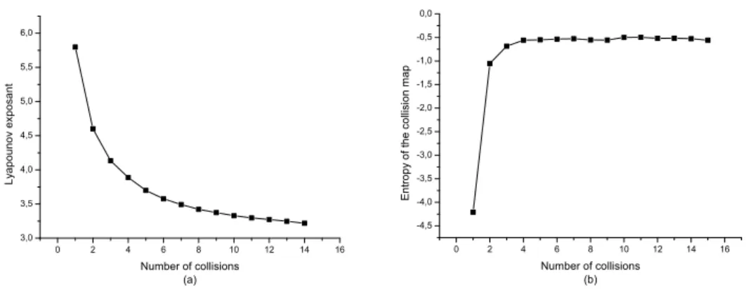
2.2 Entropy for collision map . . . 44

2.3 Spatially extended Lorentz gas entropy . . . 47

2.4 Hard disks . . . 48

2.5 Concluding remarks . . . 50

2.6 Appendix . . . 52

2.6.1 Collision Map . . . 52

2.6.2 Algorithm description . . . 53

II

Unstable Quantum Systems

57

3.8.2 Generalized Fourier transforms . . . 66

3.9 Laplace transforms . . . 67

4.1 Density matrix . . . 71

4.2 Quantum Liouville equation . . . 72

4.3 Projection operator . . . 73

4.4 Density matrix of bipartite system . . . 74

4.5 Quantum entanglement . . . 74

4.5.1 Introduction . . . 74

4.5.2 Entanglement States . . . 76

4.6 Schmidt decomposition theorem . . . 76

4.7 von Neumann entropy . . . 77

4.8 Decoherence . . . 78

4.8.1 Definition . . . 78

4.8.2 Decoherence free subspace . . . 79

5 Quantum Decay Models (I) 81 5.1 Weisskopf-Wigner theory . . . 81

5.2 Lee-Oehme-Yang theory (LOY) . . . 83

5.2.1 Mass-Decay Matrix . . . 83

5.2.2 CP violation . . . . 84

6 Two-level Friedrichs model and kaonic phenomenology 87 6.1 Introduction . . . 88

6.2 Main features of kaon phenomenology. . . 88

6.3 Friedrichs’s model and kaon phenomenology . . . 92

6.3.1 The two-levels Friedrichs model . . . 92

6.3.2 The two-levels Friedrichs model and kaonic behavior . . . 93

6.4 Conclusions. . . 97

7 Quantum-mechanical decay laws in the neutral kaons 99 7.1 Introduction . . . 100

7.2 The two-level Friedrichs model. . . 102

7.3 Main features of kaon phenomenology. . . 103

7.4 Friedrichs’s model and kaon phenomenology. . . 107

7.4.1 Solutions for v(ω) = e−αω2_/2 , α > 0, α → 0 . . . 107

7.5 Discussion of other approaches. . . 111

8 Quantum Decay Models (II) 117

8.1 One-level Friedrichs model . . . 117

8.2 Two-level Friedrichs model . . . 119

8.3 Quantum Zeno effect (QZE) . . . 120

8.4 Time operator in quantum mechanics . . . 124

8.4.1 Definition . . . 125

8.5 Time asymmetry in quantum mechanics . . . 130

8.5.1 Rigged Hilbert Space (RHS) . . . 130

8.5.2 Breit-Wigner energy distributions . . . 131

8.5.3 Lippmann-Schwinger kets representations in Hardy space . . . 133

8.5.4 Time evolution of Gamow vector . . . 135

8.5.5 Summary . . . 138

9 Decay of quantum-mechanical unstable systems and spectral projec-tions of time operator in Friedrichs model 139 9.1 Introduction . . . 140

9.2 A formula for the spectral projection of time operator . . . 143

9.3 One-level Friedrichs model . . . 145

9.4 Computation of spectral projections of T in a Friedrichs model . . . . 148

9.4.1 The case s = 0 . . . 150

9.5 Short time behavior of survival probability . . . 152

9.6 Asymptotical behavior of the survival probability for t = −s → ∞ . . 153

9.7 Conclusion . . . 154

9.8 Appendix A . . . 155

9.9 Appendix B . . . 157

9.10 Appendix C . . . 159

Dans cette th`ese, nous ´etudions un mod`ele de d´esint´egration (decay) d’un syst`eme quantique `a plusieurs niveaux appel´e le mod`ele de Friedrichs. Dans un premier tra-vail, nous consid´erons un couplage d’un kaon avec un environnement d´ecrit par un

continuum d’´energie. On montre que les oscillations du kaon entre les ´etats K1, K2,

leur decay et la violation CP sont bien d´ecrits par ce type de mod`ele. Ensuite, nous appliquons `a ce mod`ele le formalisme de l’op´erateur de temps qui d´ecrit la r´esonance, c’est-`a-dire la probabilit´e de survie des ´etats instables. Enfin, nous consid´erons un gaz de Lorentz comme un ensemble de boules de billard avec des collisions ´elastiques contre des obstacles et un syst`eme de sph`eres dures en dimension 2. Nous ´etudions la simulation num´erique de la dynamique du syst`eme et calculons l’augmentation de l’entropie de non-´equilibre au cours du temps sous l’effet des collisions et sa relation avec les exposants de Lyapounov positifs.

In this thesis, we first study Lorentz gas as a billiard ball with elastic collision with the obstacles and a system of hard spheres in 2-dimensions. We study a numerical simulation of the dynamical system and we investigate the entropy increasing in non-equilibrium with time under the effect of collisions and its relation to positive Lyapounov exponents. Then, we study a decay model in a quantum system called Friedrichs model. We consider coupling of the kaons and environment with continuous energies. Then, we show that this model is well adapted to describe oscillation, regeneration, decay and CP violation of a kaonic system. In addition, we apply in the Friedrichs model, the time super-operator formalism that predicts the resonance, i.e. the survival probability of the instable states.

I wish to express my sincere gratitude to Maurice Courbage, my supervisor, for his guidance and support throughout my thesis. I am extremely grateful to members of the thesis committee. Arno Bohm accepted to be the president of the jury and he changed his travel schedule to participate in the defense session. Tuong T. Truong accepted to be reader of my thesis and expressed his helpful comments and sugges-tions. George Zaslavsky accepted to be reader of my thesis and he let me collaborate in another research work with him and I benefited his useful remarks. Thomas Durt accepted to be a member of jury and collaborated on a part of my thesis.

I would specially like to thank Tuong T. Truong for offering me a Post-Doc in 2007-2008.

I wish to thank Pascal Monceau for his technical discussions in the numerical computation and Ilyes Kamoun for the grammatical editing of this thesis. I give my thanks to the members of the old LPTMC and MSC specially: Jean-Claude L´evy, Jean-Marc Di Meglio, Eric Huguet, Michel Pereau, Mohamed Hebache, St´ephane Metens, N¨oelle Pottier, Ardishir Rabeie, Mabrouk Zemzemi, Pedro Garcia de Leon, Tarik Garidi, Julien Queva, Avi Elkharrat, Sebastien Villain, Evelyne Authier, Carole Barache, Claudine H´eneaux, Danielle Champeau, and Nadine Beyer.

Of course, I am grateful to my wife Maryam, my parents Tayyebeh and Morteza Saberi Fathi, my brothers Mohamad Reza and Mohamad Nasser, my sister Marzieh and my family in-law for their patience and love.

Paris,

Seyed Majid Saberi Fathi June 20, 2007.

Introduction (En Fran¸cais)

0.1

Premi`

ere partie: Syst`

emes chaotiques classiques

Le th´eor`eme-H pour les syst`emes dynamiques d´ecrit l’approche `a l’´equilibre, l’irr´evers-ibilit´e et l’augmentation d’entropie pour des ´evolutions d´eterministes. L’existence de telles fonctionnelles dans les syst`emes dynamiques conservatifs a ´et´e l’objet de plusieurs investigations pendant les derni`eres d´ecennies, voir [20]- [23], [25], [28, 29, 32]). Dans ce travail, nous ´etudions ce probl`eme pour le gaz de Lorentz et les disques durs.

Le gaz de Lorentz `a deux dimensions est un syst`eme de particules sans interac-tions se d´epla¸cant avec une vitesse constante et ´etant ´elastiquement refl´echis par des diffuseurs p´eriodiquement distribu´es. Les diffuseurs sont des disques fixes. A cause de l’absence des interactions entre les particules la distribution statistique du syst`eme est r´eduit au mouvement d’une boule de billard. Nous ´etudierons l’augmentation d’entropie sous l’effet des collisions des particules avec les obstacles.

Dans la premi`ere partie de cette th`ese, nous calculerons d’abord l’augmentation d’entropie pour quelques distributions remarquables de non-´equilibre au-dessus de l’espace de phase du billard de Sina¨ı. Le syst`eme de billard est un syst`eme hyper-bolique (avec beaucoup de lignes de singularit´e) et, afin d’avoir un m´elange rapide, nous consid´ererons des distributions initiales port´ees par les fibres dilatantes. De telles mesures initiales ont ´et´e utilis´ees dans [20, 23, 32]. Pour le billard, les fibres dilatantes sont des ensembles de particules avec des vitesses parall`eles. Nous ap-pelons cette classe des ensembles initiaux un “faisceau de particules”. Nous calculons d’abord l’augmentation d’entropie en fonction des collisions pour ces derni`eres distri-butions initiales. Nous consid´ererons les obstacles uniformes finies dans l’espace de phase. Le calcul prouve que quel que soit le coarsening de ces partitions, l’entropie a

0.2 Deuxi`eme partie: “Syst`emes instables quantiques” 2

la propri´et´e monotone dans les premi`eres collisions. Il est clair que, le long du pro-cessus de m´elange, la distribution initiale se r´epartira dans toutes les cellules jusqu’`a atteindre la valeur d’´equilibre. Physiquement, ce processus est dirig´e par l’instabilit´e forte, elle est exprim´ee par l’exposant positif de Lyapounov.

Nous consid´erons ´egalement la relation du taux d’augmentation des fonctionnelles d’entropie aux exposants de Lyapounov du gaz de Lorentz. Notre calcul prouve que cette relation est exprim´ee par une in´egalit´e

max(S(n + 1) − S(n)) ≡ △S ≤Pλi≥0λi = hK−S

Autrement dit l’entropie de Kolmogorov-Sina¨ı (K − S) est une limite sup´erieure du taux d’augmentation de cette fonctionnelle.

Nous consid´ererons les syst`emes de disques durs et calculerons une fonctionnelle de l’entropie comme l’entropie spatiale sur le tore avec plusieurs cellules. Les probabilit´es sont d´efinies comme `a l’entropie de l’espace dans le gaz de Lorentz. Nous ferons ´egalement quelques comparaisons entre le th`eorem-H et la somme des exposants de Lyapounov positifs.

0.2

Deuxi`

eme partie: “Syst`

emes instables

quan-tiques”

Les syst`emes quantiques instables font l’objet de la deuxi`eme partie de cette th`ese. Nous avons employ´e le mod`ele de Friedrichs pour d´ecrire les ph´enom`enes de d´esin-t´egration (decay) dans l’espace de Hilbert et ´egalement dans l’espace de Liouville en utilisant l’op´erateur de temps.

“Ph´enom´enologie du Kaon”

G´en´eralement la m´ecanique quantique est d´ecrite par les lois unitaires d’´evolution r´eversible (par l’interm´ediaire de l’´equation de Schr¨odinger). Cette description

con-tredit notre exp´erience journali`ere o`u le vieillissement, la dissipation et l’irr´eversibilit´e

sont omnipr´esentes. Dans ce contexte, il est int´eressant d’´etudier les syst`emes quan-tiques hybrides, qui suffisamment complexes, sont en tout unitaires et dissipatifs dans des ´evolutions de temps. Ce but peut ˆetre atteint dans le cadre du mod`ele de Friedrichs.

Le mod`ele d’un niveau de Friedrichs est bien compris [57, 58, 59]: il pr´evoit que l’´etat excit´e disparaˆıt et “fond” dans le continuum. Sa probabilit´e de survie se d´esint´egre exponentiellement dans le temps. La dur´ee de vie est proportionnelle au couplage entre le mode discret et le continuum. Les syst`emes `a decroissance exponen-tielle sont tr`es communs dans la physique classique et quantique. Ils sont relativement insignifiants quand nous les consid´erons du point de vue de l’irr´eversibilit´e temporelle parce que, bien que la loi de d´ecroissance ne soit pas r´eversible au temps, de tels syst`emes se comportent comme si ils n’ont pas poss´ed´e une horloge ou une m´emoire interne : le taux de d´ecroissance est constant dans le temps, et l’´etat du syst`eme non-d´esint´egr´e reste le mˆeme `a tout moment. En g´en´eral, les syst`emes `a d´ecroissance exponentielle montrent un comportement irr´eversible mais ignorent le vieillissement. Nous prouverons que le syst`eme de deux niveaux de Friedrichs [48] permet `a d´ecrire une classe de syst`emes qui montrent des comportements riches et complexes : les oscillations, r´eg´en´erations, etc, et d´ecrit un mod`ele ph´enom´enologique relativement exact de la physique de kaons. Il y a eu plusieurs approches `a la violation de CP dans les kaons en utilisant la th´eorie de jauge (Gauge Theory) [91] ou la th´eorie de renormalisation [50]. Nous ne consid´erons pas ces aspects ici, ´egalement parce que la question est toujours partiellement ouverte aujourd’hui. Notre traitement est bas´e sur la description des syst`emes `a d´esint´egration similaires `a la g´en´eralisation de l’approche de Weisskopf-Wigner, formul´ee par Lee, Oehme et Yang (LOY) [51] dans le cas de la d´esint´egration de kaon. Plus tard, Chiu et Sudarshan [52] ont employ´e un mod`ele de Lee afin d’obtenir une correction de la th´eorie de LOY pendant des dur´ees courtes.

R´esolvant l’´equation du Schr¨odinger pour le hamiltonien, nous montrons une ´equation maˆıtresse pour la d´esint´egration des ´etats `a deux niveaux. Notre nouvelle ap-proche est bas´ee sur l’obtention d’une ´equation maˆıtresse d’un hamiltonien d´ecrivant

des modes `a d´ecroissance de (K1, K2) et non pas pour des modes de (K0_{, K}0_{) comme}

est montr´e dans la th´eorie de LOY. En supposant un faible couplage, nous obtenons une ´equation markovienne maˆıtresse qui nous permet de simuler la dur´ee de vies des kaons, aussi bien que leurs oscillations et leurs r´eg´en´erations. Il adapte mˆeme plus ´etroitement le param`etre de la destruction de la sym´etrie de CP . Dans un premier exemple, par le spectre non-born´e dans l’´energie, nous obtenons l’angle exact tan-dis que le module est 14 fois au r´esultat exp´erimental. Cependant, nous montrons qu’en utilisant les diff´erentes fonctions de coupure des degr´es continus de libert´e, nous pouvons am´eliorer l’´evaluation ci-dessus.

0.2 Deuxi`eme partie: “Syst`emes instables quantiques” 4

Nous montrons aussi, qu’il est possible d’obtenir tous les dispositifs int´eressants du mod`ele quand le hamiltonien poss`ede un spectre seulement born´e de l’inf´erieur. Dans ce cas-l`a, avec la coupure gaussienne, l’´evaluation pr´ec´edente est am´elior´ee et nous obtenons la valeur de param`etre de violation de CP qui est seulement 3 fois du r´esultat exp´erimental. Notre ´etude confirme qu’il est possible de calculer quelques dispositifs essentiels de la ph´enom´enologie tr`es riche de kaon avec un mod`ele tr`es simple tel que le mod`ele `a deux niveaux de Friedrichs. Elle confirme ´egalement que l’ingr´edient essentiel pour obtenir une dynamique de temps irr´eversible des sous-ensembles est la pr´esence des degr´es continus de libert´e d’environnement.

“Op´erateur de temps ”

Le temps appara¨ıt dans la physique principalement dans la description de mouve-ment. Mais, ce temps n’est pas celui qui correspond au changement d’´etat du temps d’un corps ou d’un syst`eme complexe. D’une part, la transformation de temps-orient´e des ´etats de syst`emes complexes est d´etermin´e comme le dispositif le plus fondamental de la thermodynamique. La deuxi`eme loi est le premier rapport faisant une distinc-tion entre le pass´e et le futur dans les processus physiques. En parlant de l’´etat d’un corps ou d’un syst`eme, nous comprenons ´evidemment un ´etat macroscopique. N´eanmoins, dans la m´ecanique quantique, la d´ecouverte des dur´ees de temps des par-ticules ´el´ementaires instables a pr´esent´e une nouvelle distinction entre le pass´e et le futur au niveau microscopique.

Dans l’autre part, nous ´etudierons les propri´et´es de la probabilit´e de survie des syst`emes quantiques instables en utilisant les projections spectrales d’op´erateur de temps ´etablies dans le cadre de la description de Liouville-von Neumann [92, 93]. Nous examinerons ces propri´et´es dans le mod`ele de Friedrichs [48]. La probabilit´e de survie devrait ˆetre une fonction de temps monotone d´ecroissante et cette propri´et´e ne pourrait pas exister dans le cadre de l’approche m´ecanique quantique habituelle [94, 95, 96]. Elle peut seulement ˆetre correctement trait´ee par un op´erateur observable de temps T dont les projections propres d´ecrivent la distribution de probabilit´e de la dur´ee de d´ecroissance.

0.3

Pr´

esentation

Cette th`ese contient quatre articles. Avant chaque article, un ou plusieurs chapitres sont consacr´es `a l’explication des th´eories appropri´ees contenue dans l’article qui suit. Dans ces chapitres, l’id´ea principale est une br´eve ´etude des th´eories. A cette fin, parfois, j’ai ´evoqu´e bri´evement une partie des r´ef´erences qui sont mentionn´es `a la fin de la section.

Dans le premier chapitre nous avons pr´esent´e quelques concepts dans les syst`emes dynamiques comme la dynamique diff´erentielle, les exposants de Lyapunov, le gaz de Lorentz et les sph`eres dures. Nous avons ´egalement fait quelques discussions sur le th´eorem de H, la th´eorie ergodique, l’entropie de Shanonn et entropie de Kolmogorov-Sina¨ı (K − S) dans le premier article “Computation of entropy increase for Lorentz gas and hard disks”, dans le chapitre 2. Dans celui-ci, nous avons d’abord pr´esent´e nos syst`emes dynamiques. Ensuite, nous avons calcul´e l’entropie pour la map de collision pour le gaz de Lorentz, et l’entropie d’espace pour le gaz de Lorentz et les disques durs.

Dans le chapitre 3, nous avons discut´e au sujet de certains pr´eliminaires math´em-atiques comme des processus de Markov, d´efinition de quelques espaces et transfor-mations. Puis, dans le quatri`eme chapitre nous avons pr´esent´e quelques concepts de m´ecanique statistique quantique comme la matrice de densit´e, l’op´erateur de projection, l’enchevˆetrement quantique (quantum entanglement), la d´ecoh´erence et l’entropie de von Neumann. La th´eorie de Wiesskopf-Wigner et la th´eorie de la Lie-Oehme-Yang (LOY) ont ´et´e discut´ees dans le chapitre 5. Le sixi`eme chapitre contient le deuxi`eme article, “Two-Level Friedrichs model and kaonic phenomenol-ogy”. Dans cet article nous avons utilis´e le mod`ele de Friedrichs sans fonction de coupure et avec l’´energie entre −∞ et +∞, pour expliquer la ph´enom´enologie de kaon et ´egalement une ´evaluation de param`etre de violation de CP . Dans le troisi`eme ar-ticle, “Quantum-mechanical decay laws in the neutral kaons”,(chapitre 7), nous avons utilis´e le mod`ele de Friedrichs avec quelques fonctions de coupure, et nos r´esultats sont tr`es proches des r´esultats exp´erimentaux.

L’effet quantique de Zeno, l’op´erateur de temps et l’asym´etrie de temps sont les autres mod`eles quantiques de H qui ont ´et´e discut´es dans le huiti`eme chapitre. A la fin, dans le dernier chapitre nous avons pr´esent´e le quatri`eme article, “Decay of quantum-mechanical unstable systems and spectral projections of time operator in Friedrichs model”, pour obtenir la probabilit´e de survie d’un syst`eme

0.3 Pr´esentation 6

instable en employant le mod`ele `a un niveau de Friedrichs. Nos r´esultats ont ´et´e pr´esent´es pour des dur´ees courtes qui ne correspondent pas `a un effet quantique de Zeno.

Publications1

- M. Courbage, S.M. Saberi Fathi; “Computation of entropy increase for Lorentz gas and hard disks”, Communications in nonlinear science and numerical simulation, 13 Issue 2 (2008) 444-455.

- M. Courbage, T. Durt, S.M. Saberi Fathi; “Two-Level Friedrichs model and kaonic phenomenology,” Physics Letters A 362 (2007) 100-104.

- M. Courbage, T. Durt, S.M. Saberi Fathi; “Quantum-mechanical decay laws in the neutral kaons,” Journal of Physics A : Math. Theor. 40 (2007) 2773-2785.

- M. Courbage, S.M. Saberi Fathi; “Decay of quantum-mechanical unstable sys-tems and spectral projections of time operator in Friedrichs model”, soumis.

- M. Courbage, S.M. Saberi Fathi; “A formula for the spectral projection of time operator”, Sera publi´e dans le proceeding of XXV Workshop on Geometric Methods

in Physics.

Conf´erences

- “Quantum Hamiltonian dynamics of the kaons phenomenology”, Chaos, Com-plexity and Transport: Theory and Applications , Marsielle June 4-8, 2007.

- “Computation of entropy increase for Lorentz gas and hard disks”, 27`eme Journ´ees de Physique Statistique, Paris, 25-26 Janvier 2007.

- “A formula for the spectral projection of time operator,” XXV Workshop on Geometric Methods in Physics, Bialowieza, Pologne, 2-8 Juillet 2006.

Introduction

0.4

First part: Classical chaotic systems

The H -theorem for dynamical systems describes the approach to equilibrium, the irreversibility and entropy increase for deterministic evolutions. The existence of such functional in measure-theoretical dynamical systems has been the object of several investigations during last decades. see [20]- [23], [25], [28, 29, 32]). Here we study this problem for the Lorentz gas and hard disks.

The Lorentz gas in two dimensions is a system of non-interacting particles moving with constant velocity and being elastically reflected from periodically distributed scatterers. The scatterers are fixed disks. On account of the absence of interactions between particles, the system is reduced to the motion of one billiard ball. We shall investigate the entropy increase under the effect of collisions of the particles with the obstacles.

In the first part of this thesis, we will first compute the entropy increase for some remarkable non-equilibrium distributions over the phase space of the Sina¨ı billiard. The billiard system is a hyperbolic system (with many singularity lines) and, in order to have a rapid mixing, we will consider initial distributions supported by the expanding fibers. Such initial measures have been used in [20, 23, 32]. For the billiard the expanding fibers are well approximated by particles with parallel arrows velocity. We call this class initial beams of particles. We first compute the entropy increase under the collision map for these initial distributions. For this, we will consider finite uniform partitions of the phase space. The computation shows that whatever the coarsening of these partitions, the entropy has the monotonic property in the initial stage. It is clear that, along mixing process, the initial distribution will spread over all cells almost reaching the equilibrium value. Physically, this process is directed by the strong instability, that is expressed by the positive Lyapounov exponent.

0.5 Second part: Unstable quantum systems 8

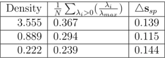
We also consider the relation of the rate of increase of the entropy functionals and Lyapounov exponents of the Lorentz gas. Our computation shows that this relation is expressed by an inequality

max(S(n + 1) − S(n)) ≡ △S ≤Pλi≥0λi = hK−S

where the ”max” is taken over n, which means that Kolmogorov-Sina¨ı (K − S) entropy is an upper bound of the rate of increase of this functional.

We shall consider the hard disks systems. We shall compute an entropy functional similar to the space entropy on extended torus with several cells. The probabilities are defined for the space entropy in the Lorentz gas. We shall also do some comparisons of the H-theorem with the sum of normalized positive Lyapounov exponents.

0.5

Second part: Unstable quantum systems

Unstable quantum systems is the second part of this thesis. We have used the Friedrichs model to describe the decay phenomena in Hilbert space and also in Liou-ville space by using the time super operator.

“Kaon phenomenology”

In general, Quantum Mechanics provides a continuous, reversible in time and unitary evolution law (via the Schr¨odinger equation). This description contradicts our everyday experience in which ageing, dissipation and irreversibility are omnipresent. In this context, it is interesting to study hybrid quantum systems, sufficiently complex, that exhibit altogether unitary and dissipative time evolutions. This goal can be achieved in the framework of the Friedrichs model.

One-level Friedrichs model is well understood [57, 58, 59]: it predicts that the excited state disappears and “fuses” into the continuum. Its survival probability decays exponentially in time. The lifetime is proportional to the coupling between the discrete mode and the continuum. Exponentially decaying systems are very common in classical and quantum physics. They are relatively trivial when we consider them from the point of view of temporal irreversibility because, although the decay law is not reversible in time, such systems behave as if they did not possess an internal clock or memory: the decay rate is constant throughout time, and the non-decayed

system is in the same state at all times. Roughly speaking, exponentially decaying systems exhibit an irreversible behavior but ignore ageing.

We shall show that the two-level Friedrichs system [48] makes it possible to de-scribe a class of systems that exhibit rich and complex behaviors: oscillations, regen-erations and so on, and provides a relatively exact phenomenological model of kaons physics. There have been several approaches to CP -violations in kaons using Gauge Theory [91] or Renormalization Theory [50]. We do not consider these aspects here, also because the question is still partially open today. Our treatment is based on the description of decaying systems similarly to the generalization of the Weisskopf-Wigner approach, formulated by Lee, Oehme and Yang (LOY) [51] in the case of kaonic decay. Later on, Chiu and Sudarshan [52] used a Lee model in order to obtain a correction to the LOY theory for short times.

Solving the Schr¨odinger equation for the Hamiltonian, we derive a master equation for the decaying two-level states. Our new approach is based on the derivation of a master equation from a Hamiltonian describing (K1, K2) decaying modes and not for

(K0_{, K}0_{) modes as done in LOY theory. Under weak coupling hypothesis this leads to}

a Markovian master equation which allows us to simulate the kaonic lifetimes as well as kaonic oscillations and regeneration. It even fits closer the CP symmetry breaking parameter. In a first example with non-bounded spectrum in energy, we obtain the exact angle while the modulus is 14 times the experimental data. However, we show that using different cut-off functions of the continuous degrees of freedom we can improve the above estimate.

We prove that it is possible to obtain all the interesting features of the model when the Hamiltonian possesses a spectrum only bounded from below. In this case, with Gaussian cut-off the previous estimate is improved and we obtain a CP violation parameter value only 3 times the experimental data. Our treatment confirms that it is possible with a very simple model such as the two-level Friedrichs model to compute some essential features of the very rich kaon phenomenology. It also confirms that the essential ingredient for deriving an irreversible in time dynamics of subsystems is the presence of a continuous degrees of freedom of environment.

“Time operator”

Time appears in physics mainly in the description of motion. But this time is not the one that corresponds to the alteration of time state of a body or a complex system. On the other hand, the time-oriented transformation of the states of complex systems is recognized as the most fundamental feature of thermodynamics. The second law

0.6 Presentation 10

is the first statement making a distinction between past and future in the physical processes. In speaking of the state of a body or a system, we obviously understand a macroscopic state. Nevertheless, in quantum mechanics, the discovery of lifetimes of unstable elementary particles has introduced a new distinction between past and future on the microscopic level.

In other hand, we shall study the properties of the survival probability of unstable quantum systems using the spectral projections of time operator built in the frame-work of the Liouville-von Neumann description [92, 93]. We shall test these properties in the Friedrichs model [48]. The survival probability should be a monotonically de-creasing time function and this property could not exist in the framework of the usual quantum-mechanical approach [94, 95, 96]. It can only be properly treated through an observable time operator T whose eigenprojections provide the probability distri-bution of the time of decay.

0.6

Presentation

This thesis contains four articles. Before each article, one or some chapters exist to explain the relevant theories. The main idea in these chapters is a short study of the theories. For this purpose, sometimes, I stated briefly a part of the references which are maintained in the end of the section.

In the first chapter we introduce some concepts in dynamical systems like, differ-ential dynamics, Lyapunov exponents, Lorentz gas and hard spheres. We also discuss about H-theorem, ergodic theory, shannon entropy and K − S entropy to introduce the first article, “Computation of entropy increase for Lorentz gas and hard disks” in the chapter 2. In this chapter, we introduce our dynamical systems. Then, we compute entropy for collision map for Lorentz gas and spatially extended Lorentz gas and hard disks entropy.

In the chapter 3, we discuss about some mathematical preliminaries like, Markov process, definition of some space and transformations. Then, in the Fourth chapter we present some concepts in the quantum statistical mechanics like density matrix, projection operator, quantum entanglement, decoherence and von Neumann entropy. The Wiesskopf-Wigner theory and Lee-Oehme-Yang (LOY) theory are discussed in chapter 5. The Sixth chapter is the second article, “Two-Level Friedrichs model

and kaonic phenomenology”. In this paper we use the Friedrichs model without cutoff function and unbounded energy to explain kaon phenomenology and also an estimation of CP violation parameter. In the third paper, “Quantum-mechanical decay laws in the neutral kaons” (chapter 7), we use the Friedrichs model with many cutoff functions, and our results are very near to experimental results.

The quantum Zeno effect, time operator and time asymmetry are the other quan-tum decay models which are discussed in the eighth chapter. Finally, in the last chapter we present the fourth article, “ Decay of quantum-mechanical unstable systems and spectral projections of time operator in Friedrichs model” to obtain the survival probability of an unstable system by using the one-level Friedrichs model. Our results present for short-time limit it is not correspond to a quantum Zeno effect.

Publications2

- M. Courbage, S.M. Saberi Fathi; “Computation of entropy increase for Lorentz gas and hard disks”, Communications in nonlinear science and numerical simulation, 13 Issue 2 (2008) 444-455.

- M. Courbage, T. Durt, S.M. Saberi Fathi; “Two-Level Friedrichs model and kaonic phenomenology,” Physics Letters A 362 (2007) 100-104.

- M. Courbage, T. Durt, S.M. Saberi Fathi; “Quantum-mechanical decay laws in the neutral kaons,” Journal of Physics A : Math. Theor. 40 (2007) 2773-2785.

- M. Courbage, S.M. Saberi Fathi; “ Decay of quantum-mechanical unstable sys-tems and spectral projections of time operator in Friedrichs model”, Submitted.

- M. Courbage, S.M. Saberi Fathi; “A formula for the spectral projection of time operator”, in proceeding of XXV Workshop on Geometric Methods in Physics, In press.

Conferences and Talks

- “Quantum Hamiltonian dynamics of the kaons phenomenology”, Chaos, Com-plexity and Transport: Theory and Applications , Marsilles June 4-8, 2007.

- “Computation of entropy increase for Lorentz gas and hard disks”, 27`eme Journ´ees de Physique Statistique, Paris, Jan. 25-26, 2007.

- “A formula for the spectral projection of time operator,” XXV Workshop on Geometric Methods in Physics, Bialowieza, Poland, July 2-8, 2006.

Part I

Chapter 1

Dynamical systems and statistical

mechanics

1.1

Differential dynamics

It is a rarity that a dynamical system can be described by mapping. The far more common case is that differential equations are required, perhaps even partial differ-ential equations. In this section, we focus on dynamical systems whose evolution is modeled by ordinary differential equations. The differential dynamical equations is of the general type

˙r = fµ(r) (1.1)

where µ is a map parameter and r ≡ {x1, . . . , xn_{} ∈ R}n_{. For example, a simple}

pendulum driven by a periodic force and subject to damping proportional to velocity, has the following Newtonian dynamics

¨

x + Ω2_{sin x = ǫ(−α ˙x + f cos ωt),} (1.2)

where ǫ, ω and f are the parameters of the system. The above equation can be written under the form of (1.1) in the usual way by defining a new variable y = ˙x. To

obtain the autonomous1 _{form, we let t → θ and then add dθ/dt = 1 to the differential}

system[1].

We refer to a solution of (1.1) as a trajectory depending on the given initial conditions. We also refer to the trajectories resulting from a neighborhood of initial

1_{A differential equation is called an autonomous differential equation if it is not dependent}

1.1 Differential dynamics 16

conditions as a flow.

1.1.1

Linearization

The dynamics determined by the vector field fµ(r) on the right-hand side of (1.1) can be highly nonlinear and complicated. However, as with maps, attracting sets and fixed points are of special interest. The fixed points are readily recognized as just those values of r for which fµ(r) is equal to zero. Fixed points can be stable or unstable, and so the behavior of fixed points is significant. To study this behavior we must linearize (1.1) in the neighborhood of such a fixed point.

Suppose re to be a fixed point of (1.1) (i.e. re is the solution of fµ(r) = 0), where

for the moment we suppress the map parameter µ. We now make a Taylor expansion of f(r) around re, assuming of course that f has adequate differentiability properties.

f(r) = f(re) + Df(re)(r − re) + · · · (1.3)

where Df(re) is the matrix of functions ∂fi/∂xj evaluated at the fixed point re. Since

f(re_{) = 0, for small (r − r}e) the dynamics is determined solely by the linear term.

By letting y = r − re, Df(re) = A, we have

˙y = Ay. (1.4)

We see that we can always expand the system to make it autonomous. The above equation is a valid approximation of (1.1) if only in a sufficiently small neighborhood

of the fixed point re. A specific solution of (1.4) with initial condition y0 is given by

y(t) = etA_y

0 (1.5)

and the general solution of (1.4) is obtained as linear superposition of n linearly

independent solutions of y_{i(t), i = 1, · · · , n.}

y(t) = n X

i=1

ciyi(t) (1.6)

where the n unknown constants are determined by the initial conditions. If the system is not degenerate we have

where λi, and vi_{, i = 1, · · · , n are the (possible complex) eigenvalues and the} eigen-vectors of the matrix A, respectively. If the system has degeneracies so that λ is an eigenvalue of A with multiplicity k, then we must compute the generalized eigenvec-tors. For k = 2 solve for u and v, where

Av = λv, _{(a − λI)u 6= 0, (a − λI)}2_{u = 0, (1.8)}

giving the independent solution vectors [1]

y1(t) = eλtv

y₂(t) = eλt_{[u + t(A − λI)u].} (1.9)

1.2

Lyapounov Exponents

The Lyapounov exponent or Lyapounov characteristic exponent (LCE) of a dynamical system is a quantity that characterizes the rate of separation of infinitesimally close trajectories. Quantitatively, two trajectories in phase space with initial separation

δx0 diverge

|δx(t)| ≈ eλt_{|δx0| (1.10)}

The rate of separation can be different for different orientations of initial separation vectors. Thus, there is a whole spectrum of Lyapounov exponents corresponding to the number of dimensions of the phase space. It is common to just refer to the largest one, because it determines the predictability of a dynamical system [35].

1.2.1

The Lyapounov Exponent for a map in one dimension

Consider two point x0 and x0_{+ ǫ mapped by the function f : I → I, where I ⊂ R is}

some bounded interval on the real line R. For n iterations of this map the Lyapounov exponent λ approximately satisfies the equation

ǫenλ = fn(x0_{+ ǫ) − f}n(x0). (1.11)

where fn_{(x0) = f (f (· · · (f(x}

0)) · · · )). Dividing by ǫ and taking ǫ → 0 gives

enλ = df n dx ¯ ¯ x0. (1.12)

1.2 Lyapounov Exponents 18

By taking n → ∞, then we have the definition for the Lyapounov exponent: λ ≡ lim n→∞ 1 nln ¯ ¯ ¯ ¯df n dx ¯ ¯ x0 ¯ ¯ ¯ ¯ (1.13) where dfn dx ¯ ¯ x0 = df dx ¯ ¯ xn−1 df dx ¯ ¯ xn−2· · · df dx ¯ ¯ x0 = f ′_(x n−1)f′(xn−2) · · · f′(x0) (1.14)

Thus, equation (1.13) can be rewritten as [1]: λ ≡ lim n→∞ 1 n n−1 X i=0 ln¯¯f′(xi)¯¯. (1.15)

1.2.2

Lyapounov Characteristic Exponents

In the last subsection, we introduced the concept of a Lyapounov Characteristic Exponent (LCE). In this subsection we expand the result of the previous subsection to more than one dimension. To state the problem in a more quantitative way, we consider a general smooth dynamical system

˙z = f(z) (1.16)

where z ≡ (r, v) is a phase space of the system. Note that the dynamical system represented by a differential equation the trajectories are referred to as flows. Let M denote the phase space manifold of an arbitrary system and denote a flow in M as

φt _{: M → M.} (1.17)

If one takes an initial point z0 ∈ M, then φt maps this initial point to φt(z0) ≡ z(t).

A flow is a one-parameter group of diffeomorphisms2 _{with the composition law}

φt2+t1 _{= φ}t2 _{◦ φ}t1_{. (1.18)}

Let z(t) denote the reference trajectory, and zs(t) a perturbed trajectory connected

to z(t) by a parametrized path with parameter s such that lims_→0zs(t) = z(t). The

associated tangent vector is defined by δz(t) = lim

s→0

zs_{(t) − z(t)}

s (1.19)

2_{A diffeomorphism is an invertible function that maps one differentiable manifold to another,}

Its equation of motion is obtained by linearizing (1.16),

δ ˙z(t) = D(z(t)).δz(t) (1.20)

where D(z(t)) = ∂f/∂z is the Jacobi matrix of the system [2]. Then, its solution according to (1.5) is equal to:

δz(t) = Dφtz.δz0 (1.21) where Dφtz = e Rt t0dt ′_D (z(t′ )) , (1.22)

is a derivative map on the tangent vectors, i.e. it is a map in TzM (space tangent

of M at z) onto Tφt(z)M (space tangent of M at φt(z)). In the particular case of a

periodic orbit of period tp, Dφtp

z is a mapping of TzM onto itself [4].

The composition rule (1.18) implies for Dφt

z that [1] Dφt1+t2 z = Dφ t2 φt1(z) ◦ Dφ t2 z (1.23)

Now, we define the LCE of δz0 ∈ Tz₀M as:

λ(z0, δz0) = lim t→∞ 1 t ln kδz(t)k kδz0k (1.24)

where k.k denotes the Euclidean norm on TzM .

Oseledec’s multiplicative ergodic theorem [3] states that for ergodic systems under very general assumptions, λ exists and that in L-dimensional phase space there are

L orthonormal initial vectors δz0 _{yielding a set of n exponents {λ}l}, which is referred

to as the Lyapounov spectrum of the system. The exponents are taken to be ordered,

λ1 _{≥ λ}2 ≥ · · · ≥ λL. Since, according to Oseledec, the λl are independent of the

metric and the initial condition, we can drop the argument z0 [2]. By using (1.21),

the equation (1.24) can be written as:

λ(z0, δz0) = lim t→∞ 1 t ln kDφ t zk (1.25)

Geometrically the Lyapounov exponents can be interpreted as the mean exponen-tial growth rates of the principal axes of an infinitesimal ellipsoid surrounding a phase point and evolving according to (1.11). Thus the Lyapounov spectrum describes the stretching and contraction characteristics of the phase flow .

1.2 Lyapounov Exponents 20

The Lyapounov exponents of the class of symplectic systems3_{, to which our hard}

particles belong if in equilibrium, exhibit a Smale-pair symmetry, λl + λ_L+1−l = 0,

for l = 1, ..., L. Furthermore, for each quantity conserved by the equations of motion one Lyapounov exponent vanishes. In a d-dimensional equilibrium system of N hard particles and phase space dimension L = 2dN the total momentum, the total (kinetic) energy, and the center of mass coordinates are conserved. Since also one exponent associated with a displacement in the flow direction equals zero, altogether 2d + 2 Lyapounov exponents vanish in this case.

Nonequilibrium steady-state systems cease to be symplectic and become dissipa-tive. Nevertheless, the Smale-pairing symmetry is not totally lost for homogeneous systems for which conjugate pairs of exponents add up to a constant negative value. Negative total sum of all Lyapounov exponents corresponds to irreversible entropy production. Furthermore, it can be shown that the sum of all Lyapounov exponents can be related to the respective macroscopic transport coefficients. The number of vanishing exponents due to the conserved quantities-center of mass, momentum, and kinetic energy-in the nonequilibrium case is a more subtle question [2].

Let δz1

0, . . . , δzk0, 1 ≤ k ≤ L, be the parallelepiped generated by the linearly

independent vectors δz1

0, . . . , δzk0 belonging to TzM . We denote the corresponding

k-dimensional volume by Vk_(δz1 0, . . . , δzk0). The limit λk(z0, δz1₀, . . . , δzk₀) = lim t→∞ 1 t ln V k_(Dφt_z(δz1 0), . . . , Dφtzδzk0) (1.26)

where λk _{are LCE’s of order k.}

For almost all vectors δz1

0, . . . , δzk0, 1 ≤ k ≤ L belonging to TzM , one has [4]

λk(z0, δz1₀, . . . , δzk₀) = k X

i=1

λi(z0), k = 1, . . . , L (1.27)

1.2.3

Numerical computation of Lyapounov spectra

The practical computation of Lyapounov spectra according to the classic algorithm of Benettin et al. [4] proceeds by simultaneously solving the original equations of motion (1.11) for the reference trajectory z(t) and the linear variational equations (1.20) for a complete set of offset vectors δz(t), The difficulties associated with the choice of

the generally unknown initial vectors δz0 and the rounding-error off effects of the

computer are overcome by periodic reorthonormalization of the set of offset vectors, such that the Lyapounov exponents are obtained from the time averaged logarithms of the respective normalizing factors. The classical method of Benettin et al. [16] can be straightforwardly applied to differentiable dynamical systems. In principle

the LCE’s of any order k could be obtained by choosing randomly k vectors in TzM

and applying definition (1.25). Practically, naive application of the definition is not possible, because in general, in the stochastic region, the vectors become too large and the angles between their directions too small to allow a numerical computation of volumes. The procedure which follows overcomes these difficulties.

Choose δz1

0, ..., δzk0 orthonormal and fix at not-too-large time τ . The idea is to

replace, at regular time intervals τ , the evolved vectors by new orthonormal vectors,

using, the Gram-Smith procedure. Precisely, denoting vi

0 = δzi0, i = 1, ..., k, one

defines and computes recursively ˜ v_li = Dφτ_φ(l−1)τ_(z)(vi_l−1) αi l = k(˜vil)⊥k vi l = k(˜v i l)⊥k αi l (1.28) where (˜vi

l)⊥stands for the component of ˜vliorthogonal to all the (already orthonormal)

v_lj with j < i, i.e., (˜vi_l)_⊥ = ˜v_li, i = 1 (˜vi_l)_⊥ = ˜v_li₋ i−1 X j=1 hvlj.˜viliv j l, i > 1, (1.29)

where h.i is the Euclidean scalar product on TzM . It is then not to difficult to prove,

using the linearity of Dφt

z and relation (1.27), that one has [4]

λi(z0) = lim L→∞ 1 nτ n X l=1 ln αi_l. (1.30)

1.3

Hard spheres model

Hard spheres are the hard balls of radii {a1, a2, . . . , aN_{} and of masses {m}1, m2, . . . , mN_},

1.3 Hard spheres model 22

free flights between binary collisions which are elastic and instantaneous. Energy and the total linear momenta are conserved [26], i.e.

mivi + mjvj = miv′i+ mjv′j (1.31) 1 2miv 2 i + 1 2mjv 2 j = 1 2miv ′2 i + 1 2mjv ′2 j . (1.32)

where vi _{≡ v}i(tn) and v′

i ≡ v′i(tn) are the velocity of ith hard balls before and after

nth _{collision in time tn respectively. Now, we rewrite the above equations as:}

       v′ ik = vik, v′ jk = vjk, mivin+ mjvjn= mivin′ + mjvjn′ , (1.33) and 1 2miv 2 in+ 1 2mjv 2 jn= 1 2miv ′2 in+ 1 2mjv ′2 jn (1.34)

where the indices ”k” and ”n” are indicates to the velocities components parallel to and perpendicular on surface at the collision point. Then, the above equations yield

             v′ ik = vik, v′ jk = vjk, v′ in = 2mj mi+mjvjn+ mi−mj mi+mjvin = vin− 2mj mi+mj(vin− vjn), v′ jn = m2mi+mijvin+ mj−mi mi+mjvjn= vjn+ 2mi mi+mj(vin− vjn). (1.35)

Finally, in the vectorial form they can be written as    v′ i = vi− 2mj mi+mj(n.vij)n v′ j = vj +m2mi+mij(n.vij)n (1.36)

where vij = (vi_{− v}j) and n =

r_i−rj

|ri−rj|, the unit vector perpendicular to surface at the

collision point (in the collision point |ri− rj| = ai+ aj).

The free flight between binary collisions are obtained as:

ri(tn) = r′_i(t_n−1) + (tn_{− tn−1})v′_i(t_n−1) (1.37)

where the indice ” ′ _{” is indicated after collision. Noting that:}

and

vi(tn) = v′_i(t_n−1) (1.39)

Now, for obtaining the LCE we must calculate the offset vector before and after collision. Thus, we take the differential from equations (1.36)-(1.39), for position we have,

δri(tn) = δr′i(tn−1) + (tn− tn−1)δv′i(tn−1) (1.40)

where δr′

i on time tn can be defined as vi△t by multiply equation (1.36) on △t we

obtain, _   δr′ i(tn) = δri(tn) − 2mj mi+mj(n.δrij(tn))n δr′ j(tn) = δrj(tn) + m2mi+mij(n.δrij(tn))n. (1.41)

where δrij = (δri _{− δr}j). For the velocities we also have,

   δv′ i(tn) = δvi(tn) − 2mj

mi+mj[(δn.vij(tn))n + (n.δvij(tn))n + (n.vij(tn))δn]

δv′

j(tn) = δvj(tn) −m2mi+mi j[(δn.vij(tn))n + (n.δvij(tn))n + (n.vij(tn))δn]

(1.42)

and

δvi(tn) = δv′_i(t_n−1). (1.43)

where δvij = (δvi_{− δv}j), and

δn = 1

a1+ a2(δrij(tn) + vij(tn)δtc). (1.44)

Here δtc is the delating time respect to the reference trajectory by [2]

δtc_{= −}n.δrij(tn).

n.vij(tn)

(1.45) The next chapter will consider the hard spheres in two dimensions (hard disks) with the same masses.

1.4 Lorentz gas 24

1.4

Lorentz gas

By considering the following assumptions for the hard balls described in the last section, we can define the Lorentz gas

             mi _{→ ∞,} ai → a, mj _{→ m,} aj _{→ 0.} (1.46)

These assumptions are that the ith _{hard ball (with infinite mass and radius ai = a)}

is fixed and the j hard ball (with mass mj = m and radius aj = 0) is a punctual. In

our simulation in the next chapter we consider all fixed hard balls (for this reason we

have chosen mi _{= ∞) in two dimensions that are distributed periodically.}

1.5

H

_-theorem

First, we start by the Boltzmann transport equation: ¡ ∂ ∂t + v1.∇r+ F m.∇v1 ¢ f1 = Z dΩ Z d3v2_σ(Ω)|v1 − v2|(f2′f1′ − f2f1) (1.47)

where σ(Ω) is the differential cross section for the collision {v1, v2_{} → {v}′

1, v′2}, Ω is

the angle between (v2_{− v}1) and (v′

2− v′1), the prim index is indicated after collision,

and

f1 _{≡ f}1(r, v1, t)

f2 ≡ f1(r, v2, t)

f₁′ _{≡ f1}′(r, v′₁, t) (1.48)

f₂′ _{≡ f}1(r, v′₂, t),

are the distributions functions. The equation (1.47) is a nonlinear integro-differential equation for f . The equilibrium distribution function of the equation (1.47) is a time independent function f0(v) that is the limit of distribution function as time goes to infinity. Assume that there is no external force. Thus, the distribution function is independent of r, i.e. f (v, t). The equilibrium distribution function,denoted by f0(v),

is the solution of the equation ∂f0(v)/∂t = 0. The Boltzmann transport equation (1.47) for f0(v) satisfies the following integral equation

0 = Z dΩ Z d3_{v2σ(Ω)|v1− v2|(f0(v}′ 2)f0(v′1) − f0(v2)f0(v1)) (1.49)

where v1 is a given velocity. The above equation yields:

f0(v′₂)f0(v′_{1) − f}0(v2)f0(v1) = 0. (1.50)

To show that the necessity of (1.50), we define the following functional: H(t) ≡

Z

d3vf (v, t) log f (v, t) (1.51)

where f (v, t) is the distribution at time, satisfying

∂f (v1, t) ∂t = Z dΩ Z d3v2_σ(Ω)|v1− v2|(f2′f1′ − f2f1) (1.52) Differentiation of (1.51) yields dH(t) dt = Z d3v∂f (v, t) ∂t [1 + log f (v, t)] (1.53)

Therefore, the condition ∂f /∂t = 0 is necessary for dH/dt = 0. Now, we see that the statement dH/dt = 0 is the same as (1.50). It would then follow that (1.50) is also a necessary condition of (1.49).

Boltzmann’s H -Theorem: If f satisfies the Boltzmann transport equation, then

dH(t)

dt ≤ 0. (1.54)

Proof: By substituting (1.47) in (1.53) we obtain dH(t) dt = Z d3v1 Z d3v2 Z dΩσ(Ω)|v1− v2|(f2′f1′ − f2f1)[1 + log f1]. (1.55)

The above integral is invariant under changing v1 and v2 because σ(Ω) is invariant

under this interchanging. We now write the above formula as follows dH(t) dt = 1 2 Z d3v1 Z d3v2 Z dΩσ(Ω)|v1− v2|(f2′f1′ − f2f1)[2 + log(f1f2)]. (1.56)

1.6 Ergodic Theory 26

This integral is invariant under interchanging {v1, v2_{} and {v}′

1, v′2} because for each

collision there is an inverse collision with the same cross section. Hence dH(t) dt = 1 2 Z d3v₁′ Z d3v′₂ Z dΩσ′_(Ω)|v′_{1− v}′_2|(f2f1− f2′f1′)[2 + log(f1′f2′)]. (1.57) By noting d3_v′

1d3v2′ = d3v1d3v2, |v′1 − v′2| = |v1− v2|, σ′(Ω) = σ(Ω) and taking the

sum of two last equation we obtain dH(t) dt = 1 4 Z d3v1 Z d3v2 Z dΩσ(Ω)|v1− v2|(f2′f1′ − f2f1)[log(f1f2) − log(f1′f2′)]. (1.58) The integrand is always negative. dH(t)/dt = 0 only if integrand becomes zero i.e. (f′

2f1′− f2f1) = 0, or under an arbitrary initial condition f (v, t) → f0(v) as t → ∞[5].

H -theorem asserts that, if at any instant the value of a certain function H, a

prop-erty of a system or of an ensemble associated with the system, is much greater than the minimum value of H, this value is very likely to decrease, although fluctuations away from the minimum value may occur; the minimum value of H is that which pos-sessed a stationary ensemble of systems, and thus is the equilibrium value. Thus, the H-theorem is a statistical theorem that gives an expression of the irreversibility char-acteristic of macroscopic system in terms of a quantity which is a microscopic analogue of the negative generalized entropy of a system in nonequilibrium thermodynamics[6].

1.6

Ergodic Theory

Why are election polls often inaccurate? Why is racism wrong? Why are your assumptions often mistaken? The answers to all these questions and to many others have a lot to do with the non-ergodicity of human ensembles. Many scientists agree that ergodicity is one of the most important concepts in statistics. So, what is it?

Ergodicity is usually described in terms of objective properties of an ensemble of objects, and the discussion often gets lost in mathematical subtleties and thus it is often difficult to understand. Nonetheless, it will be described in bayesian, subjectivist terms; hopefully this will make the concept very accessible.

Suppose you are concerned with determining what the most visited parks in a city are. One idea is to take a momentary snapshot to see how many people are at this moment in park A, how many are in park B and so on. Another idea is to look at one individual (or few of them) and to follow him for a certain period of time, e.g. a

year. Then, you observe how often the individual is going to park A, how often he is going to park B and so on.

Thus, you obtain two different results: one statistical analysis over the entire ensemble of people at a certain moment in time, and one statistical analysis for one person over a certain period of time. The first one may not be representative for a longer period of time, while the second one may not be representative for all the people. The idea is that an ensemble is ergodic if the two types of statistics give the same result. Many ensembles, like the human populations, are not ergodic [7].

1.6.1

Introduction

The first aim of ergodic theory in statistical mechanics is to determine the conditions in which the methods of statistical mechanics can be used to describe dynamical systems.

In the exact dynamical description, a single macroscopic state corresponds to many microscopic states. Thus, with exactly solving the simultaneous equations of motion

of, 1024 _{particles could be handled. Also, if the experimental measurements could}

be carried out with accuracy sufficient to yield a complete set of initial conditions for this equations, the solution gives a purely dynamical description of the system. But the thermodynamical description of a macroscopic system is characterized by the comparatively small number of parameters (which normally are the averages of the microscopic dynamical parameters) needed to specify completely the thermody-namic state of the system. Statistical mechanics uses ensembles, in order to calculate thermodynamical properties of a single system. The corresponding properties at one instant of each ensemble of systems are averaged over this ensemble; these ensemble averages represent the properties of the single system. It is clear that is not exact calculation; not only it neglects the weak interaction between particles and but also it uses some form of approximation. But, the importance of statistical elements is in the calculation of various thermodynamical properties. As regards these properties of statistical mechanics is far from being a mere substitute for exact mechanics. But, in fact, it has a much more positive significance.

Introducing some form of statistical technique is required in passing from a dy-namical to thermodydy-namical description of a macroscopic system. Ergodic theory accepts the dynamical description as basic, and it seeks conditions for the dynami-cal system to exhibit those thermodynamidynami-cal properties that may be represented by

1.6 Ergodic Theory 28

ensemble averages.

The general procedure of statistical mechanics is the Boltzmann method which it is concerned with a single dynamical system and uses statistical methods to make cal-culation pertaining to such a system. On the other treatment introduced by Gibbs, consider a collection of similar systems, together with an appropriate distribution function, and calculates averages over such ensembles of systems; the statistical con-siderations are thus much more fundamental in this approach. Gibbs, however, re-frained on the whole from attributing physical significance to his concept of an en-semble, and regarded the behavior of an ensemble of systems as being but formally analogous to that of a single physical system. Ergodic theory, or at any rate, the main body of ergodic theory, is grounded firmly on the microscopic dynamical description of a single macroscopic system; it is from this that the statistical description has to be deduced. It is carried out therefore, for the most part, within the Boltzmann framework in which the entire theory is based on a priori statistical postulates [6].

1.6.2

Statement of Ergodic Theorem

We turn now to the principal consequence of ergodicity. A function g(ω) ( assumed to be measurable µ) is said to be invariant if g(T ω) = g(ω). If g(ω) is an invariant function which is not trivial in the sense of begin a.e. constant, then for some α the invariant set {ω : g(ω) ≤ α} has a measure strictly between 0 and 1. Thus, T is ergodic if and only if each invariant function is a.e. constant. Now, we can state the ergodic theorem as:

Theorem: If f is integrable, then there exists an integrable, invariant function ˆf

which is defined as:

ˆ f (ω) = lim n→∞ 1 n n−1 X k=0 f (Tkω) (1.59)

and such that h ˆf i = R ˆf dP = R _{f dP = hfi. If T is ergodic then ˆ}f = R _{f dP = hfi}

[8].

To explain the above ergodic theorem we consider that ˆf represents a time average,

and that hfi an averaging process, then

hfi = chfi = h ˆf i = ˆf .

the first equality is obviously true for stationary ensembles, and the second follows from the resumption that one can interchange averaging processes. But the last

equality follows only if ˆf is the same for all systems in the ensemble, and this is true only if the system is ergodic [9].

To pure mathematicians it is the existence of the time averages, subject to certain conditions, that constitutes the ergodic theorem; to physicists, on the other hand the ergodic theorem expresses the equivalence of time averages and ensemble averages. The difference in terminology may perhaps have arisen from the fact that in the classical theory, which has been developed the more by mathematicians, it is the proof of the existence of the time averages that is the most difficult part of the above program, whereas in the quantum theory the existence of the time averages is a trivial problem, and it is determining the conditions under which these may be replaced by ensemble averages. Here the term the ergodic theorem will be used in the second sense with respect to both the classical and the quantal treatments. It should be recognized, however that this is a generic term, referring to any theorem expressing the equivalence of time and ensemble averages rather than to one specific set of conditions under which this equivalence holds. In the other words, the ergodic theorem embraces many ergodic theorems [6].

1.7

Coarse-graining

A measurement which is made on a macroscopic system, but which, although nec-essarily of limited accuracy, is thought of as being carried out instantaneously, may be referred to conveniently as an instantaneous macroscopic measurement. Groups of dynamical states indistinguishable by means of any set of instantaneous macro-scopic measurements may be termed phase cells, the number of dynamical states within each phase cell being dependent on the degree of accuracy of the instanta-neous macroscopic measurements. A set of instantainstanta-neous macroscopic measurements thus yields a description of the system which is much coarser than the microscopic, dynamical description; it approximates to the dynamical state by means of the phase cell which includes the dynamical state and to dynamical properties of the system by means of values characterizing ranges of values of the dynamical properties. This approximate determination of the microstate of the system may be thought of as an accurate determination of the instantaneous macro-state of the system, the instanta-neous macro-state being defined by the appropriate phase cell, and the approximate

1.7 Coarse-graining 30

values of the microscopic parameters may be regarded as accurate values of instanta-neous macroscopic observables, which, whether quantum or classical, possess discrete spectra. These instantaneous macro-observables are thus coarse-grained forms of the microscopic observables. It is by way of this coarse-graining that statistical concepts enter the route leading from the dynamical to the thermodynamical description of a system, since coarse-graining is equivalent to a statistical averaging over the various microscopic states in the phase cells. However, the statistical concepts enter in a very general form namely that there is no requirement anything like as strong as that of equal probabilities for all microscopic states within each phase cell. Nevertheless, unlike the time averaging, in which the averaging is carried out over states actually occupied by the system, there is here a definite introduction of ideas extraneous to the dynamical description, since in this coarse-grained description there are involved dynamical states additional to those which the system occupies at the time.

Coarse-graining, in fact, plays so large a part in the transition from dynamical to thermodynamical treatments that coarse-grained microscopic variables are very often regarded as being sufficiently close representations of macroscopic observables for the time averaging over a finite time interval to be used in characterizing the macroscopic observables; thus macroscopic observables are identified with what have been termed instantaneous macroscopic observables. As is remarked upon shortly, this permits a different interpretation of the significance of the time averaging over an infinite period with which the ergodic theorem deals.

The procedure of coarse-graining brings about a reduction in the number of pa-rameters used to handle the system theoretically, and such a reduction is necessary in passing to a thermodynamical description which uses only a small number of in-dependent macroscopic variables [6].

One it be admitted that it is with coarse-grained quantities that thermodynam-ical properties are to be associated, it follows that the fine-grained classthermodynam-ical ergodic

theorem is ˆ_{f = hfi, where accuracy of measurement is completely unlimited. What}

is of interest for thermodynamics is the coarse-grained ergodic theorem b

f = hfi (1.60)

where f represents value of instantaneous coarse-grained quantities. But even if this coarse-grained theorem can be proved, there remain certain general problems. Does the time average over an infinite period have any physical significance? Is it permissible to regard a macroscopic physical system as isolated? And how many

instantaneous macroscopic observables must be measured in order to determine the site of the phase cells? Although several attacks have been made on ergodic theory on the grounds that the proper response to both the first and the second questions is negative, it seems to be a solution of the third problem, that of defining phase cells, that ergodic theory needs most. Before such discussions are entered upon, however, one further feature may be mentioned, namely, that it is with only one type of thermodynamical variable that ergodic theory deals.

In ergodic theory external parameters of a system, such as the volume of the system and the intensifies of any fields external to the system, are assumed to have constant values, and so when the temporal behavior of the system is studied, no specific account need be taken of the dependence of the properties of the system on these external parameters. Apart from these external parameters thermodynamical observables are of one of two types. The first consists of properties that have dynam-ical, no less than thermodynamdynam-ical, import; such are, for example, the energy of the system and the pressure exerted by the system. These thermodynamical properties may be regarded as coarse-grained, and time-smoothed, forms of the corresponding fine-grained dynamical variables, and it is with such observables alone that ergodic theory deals; these are the variables the values of which are evaluated as ensemble averages in the usual practice of statistical mechanics.

The other kind of thermodynamical variable is of a specifically statistical nature, and chose variables - temperature, entropy, chemical potentials, and derivative quanti-ties, such as free energy have no significance with respect to a single microscopic state, and cannot be expressed in the form of ensemble averages of corresponding dynamical properties. Moreover, ergodic theory, or at any rate the main body thereof, is con-cerned with isolated systems, and for such systems neither temperature nor chemical potentials can be defined in the usual thermodynamical manner; it is when systems in mutual interaction are discussed that these concepts appear in thermodynamics. Although statistical mechanics, as distinct from thermodynamics, can provide formal definitions of temperature and of chemical potentials for an isolated system, entropy is the only one of these specifically statistical properties to have immediate ther-modynamical significance for an isolated system. This is not to say, however, that these specifically statistical quantities do not appear in the development of statisti-cal mechanics based on ergodic theory. A statististatisti-cal-mechanistatisti-cal entropy, identifiable under appropriate conditions with thermodynamical entropy, can be defined easily in terms of the ergodic distribution, which pertains to equilibrium situations, and

1.8 Entropy 32

can be generalized to nonequilibrium situations as well. Unlike the method of the

H -theorem, however, ergodic theory makes no use of this entropy in obtaining the

equilibrium distribution. As regards temperature, chemical potentials and other sta-tistical quantifies, these, too, although not considered in ergodic theory itself, appear when systems in mutual interaction are discussed. And in order to relate dynami-cal and thermodynamidynami-cal descriptions of a system it is important to consider such interacting systems; ergodic theory alone, insofar as it deals with an isolated sys-tem, cannot yield the required relationship, but constitutes merely the first albeit the fundamental step towards obtaining results of thermodynamical significance from a dynamical description of a system [6].

1.8

Entropy

1.8.1

Shannon entropy

There exists a quantity that measures the non-predictability degree of a determinis-tic and conservative dynamical system, it is called Kolmogorov-Sina¨ı entropy. This concept is not confused with thermodynamical entropy in nonequilibrium which is defined by information theory of Shannon. More precisely, it is a global character and uncertainly in the results of cross-graining observation in spite of it is known all precedent results. Moreover, the observation is smooth. It is depended on the instability of motion so that in some conditions K − S entropy is equal to the sum of the positive Lyapounov exponents. Instability creates the unpredictability. We memorize some concepts of information theory.

In the information theory, the information is obtained by transmission of a mes-sage. It is measured by the logarithm of the number of messages possible. For example, the message of N letters by k alphabet letters (a1, . . . , ak) = α is obtained

as: If in each message of N letters each letter ai is repeated pi-times, then this letter

is produced in the message with Ni = piN frequency. Now, P is

P = N !

N1_{! · · · N}k! (1.61)

and information is obtained by the transmission of a letter is:

I = log P