HAL Id: hal-00298020
https://hal.archives-ouvertes.fr/hal-00298020
Submitted on 23 Feb 2018
HAL is a multi-disciplinary open access
archive for the deposit and dissemination of
sci-entific research documents, whether they are
pub-lished or not. The documents may come from
teaching and research institutions in France or
abroad, or from public or private research centers.
L’archive ouverte pluridisciplinaire HAL, est
destinée au dépôt et à la diffusion de documents
scientifiques de niveau recherche, publiés ou non,
émanant des établissements d’enseignement et de
recherche français ou étrangers, des laboratoires
publics ou privés.
Continuous in situ measurement of quenching
distortions using computer vision
Stéphane Claudinon, Pascal Lamesle, Jean-José Orteu, Roland Fortunier
To cite this version:
Stéphane Claudinon, Pascal Lamesle, Jean-José Orteu, Roland Fortunier. Continuous in situ
mea-surement of quenching distortions using computer vision. Journal of Materials Processing Technology,
Elsevier, 2002, 122, p. 69-81. �hal-00298020�
Continuous in situ measurement of quenching distortions using
computer vision
S. Claudinon
a,1, P. Lamesle
a, J.J. Orteu
a, R. Fortunier
b,*aEcole des Mines Albi, Centre Mate´riaux, Campus Jarlard, 81013 Albi Cedex 9, France bENSM-SE, Centre SMS, 158 Cours Fauriel, 42023 Saint-Etienne Cedex 2, France
Abstract
A heat treatment vacuum furnace equipped with a CCD camera is used to follow the shape evolution of two axisymmetric steel samples during gas cooling. The experimental results are compared with numerical simulations performed with the finite element technique. A good agreement is obtained between the theoretical predictions and experiments. The shape evolution of metallic samples are measured experimentally and simulated numerically during all the cooling processes. The accuracy of the measurement is 0.01 mm, while the dimensions of the samples are 40 mm diameter and 80 mm height. Stepwise increasing hole diameters are used in the samples to amplify the shape changes during quenching. The first steel sample does not exhibit phase changes during cooling. The shape evolution is only due to thermal shrinking. Since residual distortions are not observed, the thermal gradients generated during these experiments are not large enough to induce plastic deformation.
The second steel sample presents a martensitic transformation during cooling. The shape changes are thus due to both thermal shrinking and phase changes. The residual distortions observed can be attributed to transformation plasticity. It turns out that this physical phenomenon can be studied by the experimental set up described in this paper. #
Keywords: Quenching; Distortions; Measurements; Computer vision
1. Introduction
Microstructures and residual stresses are often generated into metallic components by applying a heat treatment process. For example, quenching of steel increases hardness and produces compressive residual stresses near the surface. However, these processes may lead to permanent shape changes of the component, which are mainly due to the plastic deformation induced by thermal gradients and phase changes during the treatment [1]. A lots of work has been carried out to model the development of microstructures, stresses and strains during quenching [2 9]. In these models, most of the physical phenomena occurring during the pro cess, e.g. non isothermal phase changes, transformation plas ticity, etc., are taken into account. These models have been introduced into numerical simulation tools based on the finite element technique, so that it is now possible to predict the microstructures, stresses and strains produced during the heat treatment of metallic components with complex geometry.
Comparing the theoretical predictions with experimentally obtained microstructures, stresses and strains have validated these models. In general, a relatively good agreement is observed between experimental and calculated microstruc tures, stresses and strains obtained at the end of the heat treatment (e.g. residual stresses, distortions, etc.).
However, when a risk of distortions or cracks during quenching is detected for a given industrial component, numerical simulations are not systematically performed to quantify it. To the authors’ knowledge, the main reason is that the models involved require a very large amount of data, such as the phase transformation curves, mechanical properties of each constituent, heat exchange coefficients, etc. Moreover, the consequences of the use of any simplified set of data on the numerical results are not clearly understood. For exam ple, it is known that, during the cooling part of the quenching process, distortions occur at high temperature (at the begin ning of cooling), while residual stresses essentially develop at low temperature (at the end of cooling). Nevertheless, the influence of high and low temperature parameters on residual distortions and stresses, respectively, has not yet been quan tified. It turns out that, before any numerical simulation of a quenching process, a long time period is often necessary to
*Corresponding author.
1Now at: RENAULT, Dir. de la me´canique, 67 rue des bons raisins, 92500 RUEIL-MALMAISON.
collect the complete set of data which has to be entered into the computer software.
Numerical results can be obtained during all the quenching process, while experiments are mainly concerned with the end of it. As a consequence, continuous measurement of distor tions during a quenching process appeared to be a well suited method for analysing the efficiency of the high temperature models involved in the numerical simulations, and for quan tifying the role of the high temperature data used by these models. Some experiments have been developed in order to monitor the deformation history of materials throughout a quenching process, mostly water spray or water cooling [10,11]. However, these experimental set ups are limited to basic geometry like bars or plates. In this paper, we describe a new experimental set up aimed at following the distortions of a metallic sample during a quenching process.
In Section 1, the experimental device is described in detail. An artificial vision technique is employed to deter mine the shape of the specimen during the process. This paper then focuses on the accuracy of the measurements obtained with this technique. After that experimental results on quenching of two steel grades illustrate the use of this experimental device, and numerical simulations of these quenching processes are performed. Finally, observed dis tortions are compared with theoretical shapes predicted by the finite element technique. It is shown that the numerical simulations are generally in relatively good agreement with the experiment and that some high temperature data play a significant role on the development of distortions during quenching. This paper summarises the work described in [12], and more experimental results can be found in [13].
2. Experimental set-up
The heat treatment vacuum furnace described in Fig. 1 has been designed to monitor distortions during quenching
by computer vision. It can be seen in this figure that the primary vessel is separated into two zones. In the upper part, the samples are heated to the austenitic temperature. In the lower part, the samples are cooled to the room tempera ture by using a straight through flow of inert gas (i.e. nitrogen or helium) with an overpressure up to 5 bars. A pneumatic jack transfers the workload support, and thus the sample, between the two zones. The sample is first placed on the workload support in the gas quenching zone, which is at room temperature. Then, it is moved up to the heating zone which is under vacuum. After heating, the sample is brought back to the quenching zone for gas cooling. The dimensions of the specimen must be less than 100 mm! 100 mm ! 100 mm.
The gas quenching zone in Fig. 1 is detailed in Fig. 2. The shape variations during cooling of the specimen can be observed through the four quartz made windows distributed on the section of this zone. With a single camera (Fig. 2a), the shape variations of an axisymmetric sample can be determined by monocular vision and contour detection methods [13]. If two cameras are placed around the furnace (Fig. 2b), the 3D displacement of the surface points of the sample can be obtained by stereovision and correlation techniques [14]. Although both techniques have been devel oped, this paper is concerned with the monocular vision described in Fig. 2a. The accuracy of the results obtained with the stereovision system is currently being confirmed by further experiments.
A digital CCD camera with 1280 pixel! 1024 pixel resolution is used to monitor shape variations during cool ing. This camera is equipped with a 25 mm lens, and an acquisition card is installed on a PC computer. Finally, a filter is adapted on the lens, in order to limit sensor’s saturation due to the infrared radiation emitted by the sample (particularly above 8008C). It can be seen in Fig. 3 that the CCD camera is focussed on the apparent diameter Da of the axisymmetric component analysed,
whereas we want to determine its actual diameter D. The digital pictures taken during cooling are thus post pro cessed as follows:
" A contour detection algorithm is applied to determine the value of the apparent diameter Da.
" A conversion factor K is used to obtain the actual diameter Dof the sample from Da.
The applied contour detection algorithm is sketched in Fig. 4. The picture obtained from the CCD camera (Fig. 4a) is treated line by line. On each horizontal line, denoted by u, the grey level signal is used to determine two transitions between the sample and the gas quenching zone. The posi tions of these two transitions are calculated by determining,
with sub pixel accuracy, the zero crossing of the second derivative of the grey level signal (Fig. 4b). The distance between these two transitions finally gives the apparent diameter of the sample on the horizontal line considered. This contour detection algorithm is repeated on each line, leading to the evolution of the apparent diameter of the sample along its vertical axis, Da(u). The Da(u) function will be referred to as the apparent diameter profile of the sample. The numerical values obtained by the contour detection algorithm are those of the apparent diameter Dagiven in the pixel units corresponding to the CCD camera. The following procedure is used to obtain the actual diameter profile D(u) of the sample, expressed in millimetres, as a function of the apparent diameter profile Da(u):
Fig. 2. Optical measurement systems.
Fig. 3. Apparent diameter measurement (top view of the sample).
" The actual diameter Drof a sample, which is assumed constant along the axial direction, is measured mechani cally with 0.005 mm of accuracy (this accuracy takes into account the assumption that the diameter Dr is constant).
" The sample is placed into the gas cooling zone of the furnace, and a picture of it is taken from the CCD camera (the focal plane of the CCD camera is assumed to be parallel to the vertical axis of the sample).
" The apparent diameter profile Da(u) of this sample is determined in pixel units, by using the algorithm described above.
" Conversion factors K(u) between Da(in pixels) and Dr(in millimetres) are calculated by KðuÞ ¼ Dr=DaðuÞ (the mean value of the conversion factors obtained with the experiments described below is approximately 0.1 mm/ pixel).
As long as the CCD camera is not moved, the conversion factors K(u) obtained by this procedure are used to convert the measured apparent diameter profiles Da(u) into actual diameter profiles D(u) of the sample during quenching: DðuÞ ¼ KðuÞDaðuÞ.
3. Accuracy of the measurements
The conversion factors K(u) are established at room temperature, in the lower zone of the furnace, before moving the sample up (for heating) and down (for quenching), and without gas flow. It turns out that the accuracy of the measurements must take into account the following para meters:
" Repeatability, associated with the contour detection algo rithm.
" Position of the sample, which may change when the workload support is moved up and down.
" Temperature of the sample, leading to variations of con trast in the image analysed.
" Gas flow, which may modify the optical properties in the quenching zone.
3.1. Repeatability of the measurements
In order to quantify the repeatability of the measurements, the apparent profile of a 40 mm diameter cylindrical sample was determined with the contour detection algorithm described above. On each line, 20 measurements were performed, and a standard deviation was calculated. Fig. 5 depicts the standard deviation obtained on the horizontal lines of the sample. In Fig. 5a, the results are plotted versus the line number, while a histogram of these values is given in Fig. 5b. According to Fig. 5b, the standard deviation takes values between 0.02 and 0.05 pixel.
3.2. Position of the sample
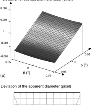
Position variations of the sample on the workload support may occur when it is moved up and down during the quenching process. These variations can be described by a translation vector t and a rotation matrix R. The translation vector contains three component (tx, ty, tz), i.e. one per space direction, while according to the axisymmetric shape of the sample, the rotation matrix can be described by two angles (y, f). Following a relatively simple geometrical analysis [12], the conversion factor K can be expressed as a function of these five parameters tx, ty, tz,y and f. This function involves the four intrinsic parameters of the CCD camera (position of the centre and aspect ratio along each direction in the image), which relate the 3D camera co ordinates to the 2D retinal image co ordinates [15]. These intrinsic para meters are determined by a classical calibration procedure.
In order to perform a sensitivity analysis of the conversion factor K against these five parameters, the limiting values of tx, ty, tz, y and f were chosen as &1 mm for the three
translation components and &0.058 for the two angles. These limiting values are somewhat arbitrary, but certainly overestimate the position changes of the sample when it is moved up and down on the workload support. As illustrated in Fig. 6, for a particular line u, these parameters have no significant influence on the accuracy of the measurement. In Fig. 6a, the variation of the apparent diameter of the sample remains less than 0.0015 pixel when the variation of the rotation anglesy and f do not exceed 0.058. In Fig. 6b, these variations remain less than 0.0016 pixel when the sample is translated along the lateral y direction.
3.3. Influence of temperature
Since the temperature of the sample modifies the form of the grey level signal used to detect its contours, this para meter must have an influence on the accuracy of the mea surements. Fig. 7 illustrates the method employed to quantify this influence. Fig. 7a gives images of the sample obtained during the cooling process. It can be seen in this figure that the grey level signal, and thus the precision of the contour detection algorithm, is highly modified by the temperature of the sample. The test model in Fig. 7b repro duces the contrast between the sample surface at different temperatures and the homogeneous background of the images. In Fig. 7c, the repeatability of the measurements on the test model is given in terms of standard deviation versus line number. In this figure, 20 measurements were carried out on each line.
According to Fig. 7, the accuracy of the measurements decreases when the surface temperature of the sample is above 8008C. It turns out that the experimental results presented in this paper are limited to surface temperatures
Fig. 6. Influence of rotation (a) or translation (b) of the sample on apparent diameter.
between 20 and 7508C. Within this range, the maximum standard deviation of the measurements is 0.1 pixel, i.e. about 0.01 mm.
3.4. Influence of gas flow
Gas flow running through the quenching zone may modify the optical properties in this zone and induce vibrations. To quantify this influence, repeatability of the measurements was tested at room temperature, with gas flow, by using the same procedure as without gas. Fig. 8 gives a histogram of the standard deviation obtained with and without gas in the quenching zone. The gas used was helium with an over pressure of 5 bars and a flow rate of 220 m3/h. It can be seen in this figure that gas flow does not have a significant influence on the accuracy of the measurement in particular, the maximum standard deviation is not changed.
4. Experimental results
According to Section 3.3, the accuracy of the measure ment system employed to follow the diameter profiles of a sample during quenching can be estimated to 0.1 pixel, i.e. about 0.01 mm, when the surface temperature of the sample is below 8008C. When the temperature is increased (above 8008C), this accuracy decreases due to a lack of contrast between the sample and the background in the image. In this section, experimental results are obtained on steel specimens. The geometry and steel grades used for the
experiments are first described. Then, the measured profiles during cooling are given and analysed.
4.1. Geometry of the samples
Steel specimens were quenched to illustrate the use of the experimental set up to follow shape changes of the samples during quenching. The particular geometry depicted in Fig. 9 was chosen to amplify distortions by producing different thermal gradients and phase transformations along the ver tical axis. A 80 mm high cylinder, with 40 mm outer dia meter and stepwise increasing hole diameters, is heated to a homogeneous temperature of 8758C for 30 min, and then quenched with helium gas under 5 bars pressure and 220 m3/ h flow rate. It is obviously expected that the upper part of the cylinder cools more rapidly than the lower part, leading to measurable variations of the outer diameter of the specimen along the vertical axis during cooling.
4.2. Steel grades
Two steel grades were used in this study, and will be referred to as specimens S1 and S2 throughout this paper. Their chemical compositions are given in Table 1. Specimen S1 is an austenitic stainless steel, and thus does not produce any phase change during quenching, while the continuous cooling transformation (CCT) diagram given in Fig. 10 indicates that phase transformations occur in specimen S2. The shape evolutions of S1 and S2 during cooling are thus expected to differ significantly.
Fig. 8. Influence of gas flow on accuracy of the measurements.
Table 1
Chemical composition of specimens S1 and S2 (wt.%)
Steel grade C Mn Si S P Ni Cr Mo
S1 X2CrNi18-9 0.030 2.00 1.00 0.03 0.045 10.00 19.00
4.3. Shape changes during cooling
For both specimens S1 and S2, the evolution of the outer diameter along the vertical axis was measured before
heating (D0value) and during cooling (D value). Figs. 11 and 12 depict the measured D'D0 profiles at different acquisition times during the cooling of specimens S1 and S2, respectively. Irregularities can be observed, which are
Fig. 9. Geometry of the specimens.
due to both specimen roughness and measurement noise. It should be noted here that the experimental results are not given:
" at the bottom of the sample, since the workload support modifies the grey level signal and the accuracy of the measurements,
" at the beginning of quenching, since the surface tempera ture of the sample is above 7508C.
It can be observed in Figs. 11 and 12 that the upper part of the specimen cools more rapidly than the lower part. More over, specimens S1 and S2 behave differently during quenching. According to Fig. 11, specimen S1 reduces in diameter by thermal shrinking during all the process, while specimen S2 shows an increase in diameter between 55 and 110 s of cooling in the upper part. At the end of cooling, specimen S1 does not exhibit any difference between the final and the initial diameter profiles, whereas specimen S2 exhibits distortions.
These first results show that:
" The cooling sequence does not generate sufficiently large thermal gradients to produce plastic deformation in the specimen S1, which does not exhibit distortions. " The phase changes in specimen S2 are clearly observed,
since they produce an increase of the outer diameter of the sample.
" The distortions observed in specimen S2 are mainly due to transformation plasticity, since thermal gradients are not large enough to produce classical plasticity.
5. Numerical simulations
The cooling part of the quenching process applied to the specimens S1 and S2 was simulated numerically by using the SYSWELD finite element computer software [16]. The aim of these simulations is to compare the experi mental results with the calculated distortions, and thus to confirm the preliminary conclusions of the previous section.
Fig. 11. Measured diameter profiles of specimen S1 during cooling.
As mentioned in the Section 1, a large amount of data is needed for quenching simulations. After describing the mesh and the boundary conditions used for the simulations, a simplified set of data is given in terms of metallurgical, thermal and mechanical properties.
5.1. Mesh and boundary conditions
The mesh used for the simulations is made of approxi mately 1800 4 nodes linear axisymmetric elements (Fig. 13), and the boundary conditions applied are:
" a heat transfer coefficient for the thermal analysis;
" the lower left node of the mesh fixed in the axial direction for the mechanical analysis.
It is assumed that the heat transfer coefficient depends neither on the steel grade nor on the inner and outer surfaces considered. As a consequence, an S1 specimen was equipped with four 0.12 mm K type thermocouples, while running through an identical gas cooling sequence as the specimens used for distortion measurements. From the measured tem perature time curves, the heat transfer coefficient was deter mined by applying a trial and error procedure using finite element calculations. The following sequence was finally defined for this coefficient:
" A linear increase from zero to its nominal value during 6 s (this time period is mainly due to the increase of gas pressure from 1 to 5 bars).
" A nominal value depending on the surface temperature: 250 W/m2/K below 5008C, 150 W/m2/K above 8008C, and a linear evolution in between.
The locations of the thermocouples are given in Fig. 14, together with the measured and calculated temperature time curves. It can be seen that the measured curves at points T3 and T4 are very close. This validates our assumption that the heat transfer coefficient is identical on the inner and outer sur faces of the sample. The main discrepancy obtained between calculated and experimental temperature time curves is 108C. Avery good agreement is thus obtained for the thermal analysis of cooling in the case of specimen S1. The same value of heat transfer coefficient is used for specimen S2. 5.2. Set of data
According to Fig. 10 (CCT diagram of S2) and Fig. 14 (involved cooling rates), it is expected that the austenite forms only martensite during cooling of specimen S2. This is confirmed in Fig. 15, which gives the martensitic micro
Fig. 13. Mesh used for the numerical simulations.
Fig. 15. Microstructure of specimen S2 after cooling.
Table 2
Material properties for specimens S1 and S2
Temperature (8C)
20 200 500 900
Young’s modulus (GPa) 200 150
Poisson’s ratio 0.29 0.31 Thermal conductivity (W/m/K) Austenite 15 27 Martensite (S2) 38 40 35 Mass enthalpy (J/kg) Austenite 160000 630000 Martensite (S2) 0 350000 Density (kg/m3) Austenite 8060 7600 Martensite (S2) 7870 7700 Thermal strain Austenite (S1) 0 0.02 Austenite (S2) 0.008 0.012 Martensite (S2) 0 0.008
Yield stress (MPa)
Austenite 40 80 70 25
Martensite (S2) 780 460
Hardening coefficient (GPa)
Austenite 3 0.5
structures obtained in the sample after cooling. Following the Koistinen Marburger equation, the proportion of mar tensite p is obtained as a function of temperature y by p¼ 1 ' exp ðbðy ' MsÞÞ when y < Ms, and p ¼ 0, other wise. The martensite start temperature Ms was found at 3008C (Fig. 10), and the kinetic coefficient b was chosen as 0.011/8C.
The material properties of S1 and S2 were taken from Refs. [3,9]. In order to simplify the data, it was assumed that austenite in S1 and in S2 have the same properties, and that the Young’s modulus and the Poisson’s ratio were not phase dependent. Moreover, linear kinematic hardening laws were used for the mechanical analyses. The data are listed in Table 2, and linear interpolations are used between the indicated values. It can also be seen in this table that the thermal expansion vanishes at 208C for austenite in speci men S1, and for martensite in specimen S2. This gives the reference value for the distortion calculations in both speci mens.
6. Discussion
The aim is to outline the possibilities of the experi mental device described in this paper. For this purpose,
the experimental results obtained in the previous section are compared with the numerical simulations.
6.1. Specimen S1 (X2CrNi18 9 steel)
Fig. 16 gives the calculated and measured D'D0profiles during the cooling of specimen S1, which is made of austenitic steel, and thus does not exhibit any phase change. Thermal shrinking can be clearly observed in this figure. The upper part of the cylinder cools faster than the lower part at the beginning of cooling, leading to a relatively large difference between the corresponding outer diameters. This difference then reduces since the temperature field becomes homogeneous. At the end of cooling, no significant distor tion is observed. This is due to the fact that the thermal gradients generated by gas quenching are not high enough in this case to produce plastic deformation in the specimen.
A very good agreement is obtained between experimental and calculated profiles during all the process. A slight discrepancy can be observed at t¼ 110 s, particularly at the bottom of the sample. It is probably due to heat exchanges between the specimen and the workload support, which were not taken into account in the calculations. It should be noted here that Fig. 16 demonstrates that the experimental device described in this paper is able to follow
Fig. 17. Calculated and measured diameter profiles of specimen S2 during cooling.
the shape of a metallic part during the cooling sequence of a quenching process.
6.2. Specimen S2 (30CrNiMo8 steel)
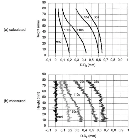
Fig. 17 gives the calculated and measured D'D0profiles during the cooling of specimen S2, which is made of a steel that presents phase changes during quenching. A good agreement can be observed between the measured and the calculated profiles. At the beginning of cooling, thermal shrinking leads to similar shapes as for specimen S1 (Fig. 16). Then, when the temperature reaches 3008C, which is the Ms value in Fig. 10, austenite begins locally to transform into martensite, and thus to generate a thermal expansion. This temperature is reached at t¼ 55 s at the top of the specimen, whereas transformation begins only at t¼ 185 s at the bottom. At the end of cooling, a slight distortion can be observed, which is mainly due to trans formation plasticity since according to specimen S1 thermal gradients do not generate classical plasticity.
These calculations and measurements can also be employed to analyse local displacements at the surface of the specimen. Fig. 18 depicts the calculated and measured displacements during cooling at two particular points of the sample. This figure confirms that martensite forms gradually from the top (e.g. point A) to the bottom (e.g. point B) of the specimen.
7. Concluding remarks
Quenching distortions of metallic components are mainly due to:
" plastic deformation, induced by thermal gradients, which is often referred to as ‘‘classical plasticity’’,
" plastic deformation, produced by phase changes, which is often called ‘‘transformation plasticity’’.
The analysis of gas quenching distortions of two steel specimens (S1, without phase changes; S2, with a marten sitic transformation) validates the experimental set up. The results are compared with numerical finite element simula tions. The main conclusions are that:
" A good agreement is observed between theoretical pre dictions and experiment during all the cooling sequence. " The shape evolution during cooling of specimen S1 is only due to thermal shrinking, and does not produce any residual distortions. The thermal gradients produced dur ing gas cooling are thus not large enough to induce classical plasticity.
" The phase changes in specimen S2 significantly modify its shape evolution during cooling, and produce residual distortions, which are clearly due to transformation plas ticity effects.
The contour detection technique described in this paper is well suited for studying samples with an axisymmetric shape. By using a stereovision method, it will be possible to analyse samples with more complex geometry.
References
[1] E. Ameen, Dimension changes of tool steels during quenching and tempering, Trans. ASM 28 (1940) 472 512.
[2] T. Inoue, S. Nagaki, T. Kishino, M. Monkawa, Description of transformation kinetics, heat conduction and elastic plastic stress in the course of quenching and tempering of some steels, Ing. Arch. 50 (1981) 315 327.
[3] S. Sjo¨stro¨m, The calculation of quench stresses in steel, Ph.D. Study, Linko¨ping University, Sweden, 1982.
[4] J.B. Leblond, J. Devaux, A new kinetic model for anisothermal metallurgical transformations in steels including effect of austenite grain size, Acta Met. 32 (1984) 137 146.
[5] F.B.M. Fernandes, S. Denis, A. Simon, Mathematical model coupling phase transformation and temperature evolution during quenching of steels, Mater. Sci. Technol. 10 (1985) 838 844. [6] T. Inoue, Z. Wang, Coupling between stress, temperature and
metallic structures during processes involving phase transformations, Mater. Sci. Technol. 10 (1985) 845 850.
[7] J.B. Leblond, G. Mottet, J.C. Devaux, A theoretical and numerical approach to the plastic behaviour of steels during phase transforma-tion. I. Derivation of general relations, J. Mech. Phys. Solids 34 (4) (1986) 395 409.
[8] J.B. Leblond, G. Mottet, J.C. Devaux, A theoretical and numerical approach to the plastic behaviour of steels during phase transforma-tion. II. Study of classical plasticity for ideal-plastic phase, J. Mech. Phys. Solids 34 (4) (1986) 411 432.
[9] A. Thuvander, Calculation of distortion during quenching of a case hardening steel, Report IM-2637, Swedish Institute for Metals Research, Institutet fo¨r Metallforskning, 1990.
[10] R. Becker, M.E. Karabin, J.C. Liu, R.E. Smelser, Distortion and residual stress in quenched aluminium bars, J. Appl. Mech. 63 (1996) 699 705.
[11] M. Oldenburg, G. Bergman, L. Sandberg, M. Jonsson, Experiments with one-sided spray-cooling of steel plates for evaluation of thermo-mechanical materials models, in: Proceedings of the Second International Conference on Quenching and Control of Distortion, Cleveland, OH, 1996.
[12] S. Claudinon, Contribution a` l’e´tude des distorsions au traitement thermique: suivi continu par vision artificielle et simulation nume´rique par e´le´ments finis, Ph.D. Study, Ecole des Mines de Paris, France, 2000.
[13] S. Claudinon, P. Lamesle, J.J. Orteu, R. Fortunier, Monitoring distortions of metallic parts during heat treatment, in: Proceedings of the Third International Conference on Heat Treatment with Atmo-spheres, ASM International Heat Treating Congress, Go¨thenburg, Sweden, 2000.
[14] D. Garcia, J.J. Orteu, 3D deformation measurement using stereo-correlation applied to the forming of metal or elastomer sheet, in: Proceedings of the International Workshop on Video-controlled Materials Testing and In situ Microstructural Char-acterisation, November 16 18, Ecole des Mines de N, Nancy, France, 1999.
[15] O. Fangeras, Three Dimensional Computer Vision A Geometric Viewpoint, The MIT Press, Cambridge, MA, 1996.