Do we have enough pieces of the jigsaw to integrate CO2 fluxes in the Coastal Ocean ?

3

Q2005 Estuarine Research Federation

Do We Have Enough Pieces of the Jigsaw to Integrate CO

Fluxes in the Coastal Ocean?

Universite´ de Lie`ge, MARE, Unite´ d’Oce´anographie Chimique, Institut de Physique (B5), B-4000 Sart-Tilman, Belgique

ABSTRACT: Annually integrated air-water CO2 flux data in 44 coastal environments were compiled from literature.

Data were gathered in 8 major ecosystems (inner estuaries, outer estuaries, whole estuarine systems, mangroves, salt marshes, coral reefs, upwelling systems, and open continental shelves), and up-scaled in the first attempt to integrate air-water CO2fluxes over the coastal ocean (263 106km2), taking into account its geographical and ecological diversity.

Air-water CO2fluxes were then up-scaled in global ocean (3623 106km2) using the present estimates for the coastal

ocean and those from Takahashi et al. (2002) for the open ocean (3363 106_km2_{). If estuaries and salt marshes are not}

taken into consideration in the up-scaling, the coastal ocean behaves as a sink for atmospheric CO2(21.17 mol C m22

yr21_{) and the uptake of atmospheric CO}

2by the global ocean increases by 24% (21.93 versus 21.56 Pg C yr21). The

inclusion of the coastal ocean increases the estimates of CO2uptake by the global ocean by 57% for high latitude areas

(20.44 versus 20.28 Pg C yr21_{) and by 15% for temperate latitude areas (}22.36 versus 22.06 Pg C yr21_{). At subtropical}

and tropical latitudes, the contribution from the coastal ocean increases the CO2emission to the atmosphere from the

global ocean by 13% (0.87 versus 0.77 Pg C yr21_{). If estuaries and salt marshes are taken into consideration in the}

up-scaling, the coastal ocean behaves as a source for atmospheric CO2(0.38 mol C m22yr21) and the uptake of atmospheric

CO2from the global ocean decreases by 12% (21.44 versus 21.56 Pg C yr21). At high and subtropical and tropical

latitudes, the coastal ocean behaves as a source for atmospheric CO2but at temperate latitudes, it still behaves as a

moderate CO2sink. A rigorous up-scaling of air-water CO2fluxes in the coastal ocean is hampered by the poorly

con-strained estimate of the surface area of inner estuaries. The present estimates clearly indicate the significance of this biogeochemically, highly active region of the biosphere in the global CO2cycle.

Introduction

The coastal ocean has been largely ignored in global carbon budgeting efforts, even if the related flows of carbon and nutrients are disproportion-ately high in comparison with its surface area (Smith and Hollibaugh 1993; Gattuso et al. 1998a; Wollast 1998; Liu et al. 2000; Chen et al. 2003). It receives massive inputs of organic matter and nu-trients from land, exchanges large amounts of mat-ter and energy with the open ocean across conti-nental slopes, and constitutes one of the most bio-geochemically active areas of the biosphere (Gat-tuso et al. 1998a). For instance, average primary production rates differ by a factor of 2 between open oceanic and coastal provinces (Wollast 1998). Although continental shelves only represent about 7% of the oceanic surface area, they account for about 20% of the total oceanic organic matter pro-duction, 80% of total oceanic organic matter buri-al, 90% of total oceanic sedimentary mineraliza-tion, and 30% and 50% of the total oceanic pro-duction and accumulation, respectively, of partic-ulate inorganic carbon (Gattuso et al. 1998a;

* Tele: 13243663187; fax: 13243662355; e-mail: alberto. borges@ulg.ac.be

Wollast 1998). Intense air-water CO2 exchanges

can be expected from such significant carbon flux-es. Human activities are changing the continental water cycle and the flows of sediment, carbon, and nutrients to the coastal ocean with likely conse-quences for the sequestration or emission of an-thropogenic CO₂(Ver et al. 1999; Rabouille et al. 2001; Mackenzie et al. 2004a,b).

The cycle of CO2 in the coastal ocean has

re-cently been put under the spotlight by the work of Tsunogai et al. (1999). These authors reported in the East China Sea an air-water CO2flux of 22.92

mol C m22 _yr21 _{that when extrapolated to the}

worldwide continental shelf area yields a sink for atmospheric CO2of20.95 Pg C yr21 that is

desig-nated as ‘‘the continental shelf pump’’ (note that Tsunogai et al. [1999, p. 701] used in their com-putation a continental shelf surface area of 27 3 106 _km2_{). It is driven by the cooling of surface}

coastal waters that leads to the formation of dense water as well as an enhancement of CO2absorption

together with high primary production. In the dense bottom waters, sedimented organic matter is degraded into dissolved inorganic carbon (DIC) that is transported along isopycnals from the con-tinental shelf to the adjacent deep ocean. The

ex-port of particulate (POC) and dissolved (DOC) or-ganic carbon from the shelf to the deep adjacent ocean across the continental shelf break is signifi-cant (e.g., Wollast 1998; Liu et al. 2000; Wollast and Chou 2001; Chen et al. 2003; Ducklow and Mc-Callister 2004) and could in theory also drive a sink for atmospheric CO2over the shelf. Although

the rate of final burial of organic matter on the continental slopes is recognized as relatively small (Wollast 1998; Wollast and Chou 2001 and refer-ences therein), the CO2produced in deep oceanic

waters from the degradation of organic matter ported from continental shelves will to a large ex-tent be ventilated back to the atmosphere in the open ocean. This leads to an underestimation of the sink of atmospheric CO2in the open ocean if

the air-water CO2 fluxes over continental shelves

are not taken into account (Yool and Farsham 2001).

If the continental shelf CO2 pump formulated

by Tsunogai et al. (1999) is confirmed worldwide, it would have major implications on our under-standing of the global carbon cycle and a signifi-cant revision of the estimate of the overall oceanic pump for atmospheric CO2. It would imply an

in-crease of 61% of the uptake of atmospheric CO2

from the oceans, since open oceanic waters are es-timated to absorb 21.56 Pg C yr21 _{(Takahashi et}

al. [2002] revised climatology for reference year 1995 available from http://www.ldeo.columbia. edu/res/pi/CO2/).

It was established more than 30 years ago, by the pioneering studies of Park et al. (1969), Kelley and Hood (1971a), and Kelley et al. (1971), that some coastal ecosystems, such as estuaries and upwelling systems, behave (at least temporally) as strong sources of CO2 to the atmosphere. A rigorous

ex-trapolation of air-water CO₂ fluxes in the coastal ocean should take into account the potential lati-tudinal variability of air-water CO2fluxes (that has

been documented in detail in open oceanic wa-ters), and, more importantly, the diversity of coast-al ecosystems with fundamentcoast-ally contrasting car-bon biogeochemical cycling.

This paper compiles current knowledge on air-water CO2 fluxes in the major ecosystems of the

coastal ocean and the main biogeochemical pro-cesses controlling them are briefly discussed. The first integration of CO2fluxes in the global ocean

including coastal and open oceanic realms is also attempted. One of the aims of this tentative up-scaling of air-water CO2fluxes in the coastal ocean

is to identify the major pieces lacking from the jig-saw to allow a better constrained global integration in the future.

SYNTHESIS

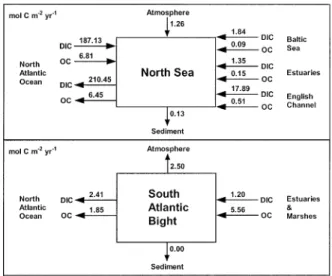
The coastal ocean is defined as the area extend-ing from the shore to the continental shelf break, excluding continental slopes but including inner estuaries. The remaining oceanic waters are re-ferred to as open ocean, the second component of what is referred to as global ocean. Data were gath-ered from literature in 8 main coastal ecosystems (inner estuaries, outer estuaries, whole estuarine systems, mangroves, salt marshes, coral reefs, up-welling systems, and open continental shelves). This list is not exhaustive but corresponds to a compromise between data availability and specific-ity of carbon cycling in these systems, and in par-ticular air-water CO2 fluxes. Table 1 summarizes

partial pressure of CO2(pCO2) and air-water CO2

flux data in 44 coastal environments (also repre-sented in Fig. 1). The majority of data in Table 1 are annually integrated CO2fluxes computed from

field data (for a detailed literature survey of CO2

data in coastal ecosystems excluding estuaries but including sites without a full annual coverage refer to Ducklow and McCallister [2004]). Air-water CO2

fluxes derived from indirect approaches (mass bal-ance calculations or numerical models) were not included in this compilation because they are prone to relatively large uncertainty. The net air-water CO₂flux is the balance of numerous biogeo-chemical processes that in most coastal ecosystems are characterized by rates that are one order of magnitude higher than the net exchange of CO₂ across the air-water interface. The most straight-forward and robust way to estimate air-water CO2

fluxes relies on field pCO2data, although this

ap-proach also suffers from the reliability of gas trans-fer parameterizations and scaling problems. Mass balance calculations or numerical models are nev-ertheless essential to understand and evaluate the relative importance of the processes responsible for air-water CO2fluxes. Values for some study sites

in Table 1 are not based on a full annual coverage, but from our understanding of carbon cycling and its seasonality in that given ecosystem, it was as-sumed that they give a reasonably good approxi-mation of the direction and intensity of annual air-water CO2 flux (in particular some sites in

man-grove surrounding waters and inner estuaries). For some sites, pCO₂ field data were compiled from different publications and the annually integrated air-water CO2fluxes computed (as explained in the

legend of Table 1).

INNERESTUARIES

At the land-ocean interface, inner estuaries re-ceive large amounts of dissolved and particulate matter, in particular organic and inorganic carbon,

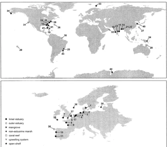
Fig. 1. Map showing location of coastal environments where air-water CO2fluxes have been satisfactorily integrated at annual

scale. Numbers indicate locations named in first column of Table 1.

and nutrients carried by rivers. These are highly dynamic systems characterized by strong gradients of biogeochemical compounds, enhanced organic matter production and degradation processes, and intense sedimentation and resuspension. Terrestri-al matter carried by rivers undergoes profound transformations in estuaries before reaching the adjacent coastal zone.

The relatively exhaustive definition of an inner estuary given by Cameron and Pritchard (1963, p. 306) was used: ‘‘a semi-enclosed coastal body of water, which has free connection with the open sea, and within which seawater is measurably dilut-ed with freshwater derivdilut-ed from land drainage.’’ The upstream boundary of the inner estuary is the limit of the tidal influence (tidal river), where wa-ter currents and sedimentary processes become drastically different from those in the river. The lower boundary of the inner estuary is the geo-graphic limit of the coast corresponding to the riv-er mouth. Because innriv-er estuaries exhibit a large diversity in terms of geomorphology, geochemistry and surface area of the drainage basin, freshwater discharge, and tidal influence, physical attributes

are affected that strongly influence biogeochemi-cal carbon and nutrient cycling, such as vertibiogeochemi-cal stratification, longitudinal gradients, spatial extent, and residence time of freshwater.

Inner estuaries are net heterotrophic systems, where total respiration (R, sum of respiration by autotrophs and heterotrophs in both benthic and pelagic compartments) exceeds gross primary pro-duction (GPP), and where net ecosystem

produc-tion (NEP 5 GPP 2 R) is ,0. Gattuso et al.

(1998a) reported an average NEP of 26 6 2 mol C m22 _yr21 _{in 21 estuaries worldwide. Caffrey}

(2004) reported an average NEP of240 6 24 mol C m22_yr21 _{in 42 United States estuaries. The}

eco-system function of inner estuaries has been modi-fied by human activities in a way that at present time is difficult to identify (Gattuso et al. 1998a; Smith et al. 2003; Gazeau et al. 2004a,b; Soetaert et al. 2004). Higher nutrient loadings due to hu-man activities may have increased NEP, while deg-radation of anthropogenic organic carbon decreas-es NEP (Gattuso et al. 1998a). Overall, thdecreas-ese eco-systems are sinks for organic matter, sources of in-organic nutrients and of CO2 to the surrounding

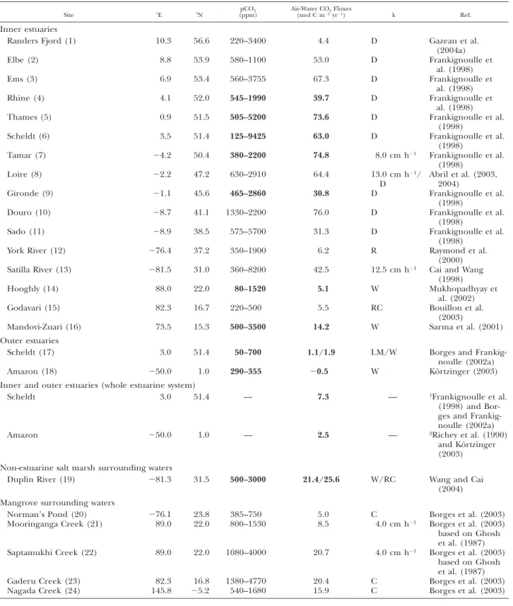
TABLE 1. Range of pCO2, air-water CO2fluxes, and gas transfer velocity parameterization (k) in coastal environments. The numbers

in parentheses correspond to site identification in Fig. 1. Values in bold are for environments with full annual coverage. k wind parameterization after Carini et al. (1996)5 C; Liss and Merlivat (1986) 5 LM; Nightingale et al. (2000) 5 N; Raymond et al. (2000) 5 R; Raymond and Cole (2001) 5 RC; Wanninkhof (1992) 5 W; Tans et al. (1990) 5 T; Wanninkhof and McGillis (1999) 5 WMcG. D denotes direct measurements with a floating dome.

Site 8E 8N pCO2

(ppm) Air-Water CO(mol C m222_yrFluxes21_{) k Ref.}

Inner estuaries Randers Fjord (1) Elbe (2) Ems (3) Rhine (4) 10.3 8.8 6.9 4.1 56.6 53.9 53.4 52.0 220–3400 580–1100 560–3755 545–1990 4.4 53.0 67.3 39.7 D D D D Gazeau et al. (2004a) Frankignoulle et al. (1998) Frankignoulle et al. (1998) Frankignoulle et al. (1998) Thames (5) 0.9 51.5 505–5200 73.6 D Frankignoulle et al.

(1998)

Scheldt (6) 3.5 51.4 125–9425 63.0 D Frankignoulle et al. (1998)

Tamar (7) 24.2 50.4 380–2200 74.8 8.0 cm h21 _{Frankignoulle et al.}

(1998) Loire (8) 22.2 47.2 630–2910 64.4 13.0 cm h21_/

D

Abril et al. (2003, 2004)

Gironde (9) 21.1 45.6 465–2860 30.8 D Frankignoulle et al. (1998)

Douro (10) 28.7 41.1 1330–2200 76.0 D Frankignoulle et al. (1998)

Sado (11) 28.9 38.5 575–5700 31.3 D Frankignoulle et al. (1998)

York River (12) 276.4 37.2 350–1900 6.2 R Raymond et al. (2000) Satilla River (13) 281.5 31.0 360–8200 42.5 12.5 cm h21 _{Cai and Wang}

(1998) Hooghly (14) 88.0 22.0 80–1520 5.1 W Mukhopadhyay et

al. (2002) Godavari (15) 82.3 16.7 220–500 5.5 RC Bouillon et al.

(2003)

Mandovi-Zuari (16) 73.5 15.3 500–3500 14.2 W Sarma et al. (2001) Outer estuaries

Scheldt (17) 3.0 51.4 50–700 1.1/1.9 LM/W Borges and Frankig-noulle (2002a) Amazon (18) 250.0 1.0 290–355 20.5 W Ko¨rtzinger (2003) Inner and outer estuaries (whole estuarine system)

Scheldt 3.0 51.4 — 7.3 — 1_{Frankignoulle et al.}

(1998) and Bor-ges and Frankig-noulle (2002a) Amazon 250.0 1.0 — 2.5 — 2_{Richey et al. (1990)}

and Ko¨rtzinger (2003) Non-estuarine salt marsh surrounding waters

Duplin River (19) 281.3 31.5 500–3000 21.4/25.6 W/RC Wang and Cai (2004) Mangrove surrounding waters

Norman’s Pond (20) 276.1 23.8 385–750 5.0 C Borges et al. (2003) Mooringanga Creek (21) 89.0 22.0 800–1530 8.5 4.0 cm h21 _{Borges et al. (2003)}

based on Ghosh et al. (1987) Saptamukhi Creek (22) 89.0 22.0 1080–4000 20.7 4.0 cm h21 _{Borges et al. (2003)}

based on Ghosh et al. (1987) Gaderu Creek (23) 82.3 16.8 1380–4770 20.4 C Borges et al. (2003) Nagada Creek (24) 145.8 25.2 540–1680 15.9 C Borges et al. (2003)

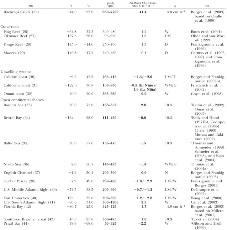
TABLE 1. Continued.

Site 8E 8N pCO2

(ppm) Air-Water CO(mol C m222_yrFluxes21_{) k Ref.}

Itacurac¸a´ Creek (25) 244.0 223.0 660–7700 41.4 4.0 cm h21 _{Borges et al. (2003)}

based on Ovalle et al. (1990) Coral reefs

Hog Reef (26) 264.8 32.3 340–480 1.2 W Bates et al. (2001) Okinawa Reef (27) 127.5 26.0 95–950 1.8 LM Ohde and van

Woe-sik (1999) Yonge Reef (28) 145.6 214.6 250–700 1.5 D Frankignoulle et al.

(1996)

Moorea (29) 2149.8 217.5 240–580 0.1 D Gattuso et al. (1993, 1997) and Fran-kignoulle et al. (1996) Upwelling systems

Galician coast (30) 29.2 42.5 265–415 21.3/22.6 LM/T Borges and Frankig-noulle (2002b) California coast (31) 2122.0 36.8 100–850 20.5 (El Nin˜o)/

1.9 (La Nin˜a)

WMcG Friederich et al. (2002)

Oman coast (32) 49.0 20.0 365–660 0.9 W Goyet et al. (1998) Open continental shelves

Barents Sea (33) 30.0 75.0 168–352 22.8 10.3 3_{Kaltin et al. (2002),}

Omar et al. (2003) Bristol Bay (34) 2164 58.0 111–450 20.6 10.3 4_{Kelly and Hood}

(1971b), Codispo-ti et al. (1986), Chen (1993), Murata and Taki-zawa (2002) Baltic Sea (35) 20.0 57.0 156–475 21.5 10.3 5_{Thomas and}

Schneider (1999), Schneier et al. (2003), and Kuss et al. (2004) North Sea (36) 2.6 56.7 145–495 21.4 WMcG Thomas et al.

(2004a)

English Channel (37) 21.2 50.2 200–500 0.0 N Borges and Frankig-noulle (2003) Gulf of Biscay (38) 27.9 49.0 260–460 21.8/22.9 LM/W Frankignoulle and

Borges (2001) U.S. Middle Atlantic Bight (39) 274.5 38.5 200–660 20.7/21.2 LM/W DeGranpre et al.

(2002)

East China Sea (40) 125 32.0 200–390 21.2/22.8 LM/W Wang et al. (2000) U.S. South Atlantic Bight (41) 280.6 31.0 300–1200 2.5 W Cai et al. (2003) Florida Bay (42) 280.7 25.0 325–725 1.7 4.0 cm h21 _{Borges et al. (2003)}

based on Millero et al. (2001) Southwest Brazilian coast (43) 245.5 225.0 350–475 1.0 10.3 6_{Ito et al. (2004)}

Pryzd Bay (44) 78.9 268.6 50–325 22.2 W 7_{Gibson and Trull}

(1999)

1_{Using a flux of 63.0 mol C m}22_yr21_{and surface area of 220 km}2_{for the inner estuary (Frankignoulle et al. 1998) and a flux of}

1.5 mol C m22_yr21_{and surface area of 2100 km}2_{for the outer estuary (Borges and Frankignoulle 2002a).}

2_{Using a flux of 164 mol C m}22_yr21_{(at Obidos, Richey et al. 1990) and surface area of 44,186 km}2_{(from the river mouth to}

Obidos, based on Chapman et al. [2002], Seyler personal communication) for the inner estuary and a flux of20.5 mol C m22_yr21

and surface area of 2.43 106_km2_{for the outer estuary (Ko¨rtzinger 2003).}

3_{Using the average k value for continental shelves of 10.3 cm h}21_{proposed by Tsunogai et al. (1999) and assuming a zero air-ice}

CO2flux (ice coverage based on data from the National Snow and Ice Data Center downloaded from http://nsidc.org/).

4_{Using the average k value for continental shelves of 10.3 cm h}21_{proposed by Tsunogai et al. (1999) and assuming a zero air-ice}

CO2flux (ice coverage based on Walsh and Dieterle [1994]).

5_{Using the average k value for continental shelves of 10.3 cm h}21_{proposed by Tsunogai et al. (1999).} 6_{Using the average k value for continental shelves of 10.3 cm h}21_{proposed by Tsunogai et al. (1999).} 7_{Assuming a zero air-ice CO}

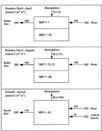
Fig. 2. Dissolved inorganic carbon (DIC) budgets for 2 cruis-es in the Randers Fjord and an annual budget in the Scheldt estuary, based on Gazeau et al. (2004a,b). Net ecosystem pro-duction (NEP) was estimated from up-scaled oxygen incuba-tions in both estuaries. In the Randers fjord, NEP was up-scaled in the upper and bottom layers. Air-water CO2fluxes are

com-puted as the closing term of the budget and compared with air-water CO2fluxes computed from pCO2 measurements

(num-bers in brackets). Note that fluxes are expressed in mmol C m22

d21_{unlike in other figures and tables.}

water, and potential sources of CO2 to the

atmo-sphere.

All the estuaries listed in Table 1 are net sources of CO2to the atmosphere, so this behavior appears

to be a general feature, although the range of re-ported air-water CO2 fluxes encompasses one

or-der of magnitude (in accordance with the recent review by Abril and Borges [2004] that also com-piles studies in estuaries where pCO2was measured

but air-water CO2fluxes were not reported).

High-ly polluted estuaries such as the Scheldt and rela-tively pristine ones such as the Satilla are oversat-urated in CO2 with respect to the atmosphere.

Among European estuaries, the Scheldt and Randers Fjord are at the higher and lower bounds, respectively, of reported air-water CO2 fluxes. In

both these estuaries a carbon budget was estab-lished from simultaneous and independent mea-surements of metabolic process rates and air-water CO2 exchanges, based on the results from the

re-cent European Union project EUROTROPH (Fig. 2). The Randers Fjord is a microtidal estuary

char-acterized by a strong permanent stratification, while the Scheldt estuary is a macrotidal estuary characterized by a permanently well-mixed water column. Although on the whole the Randers Fjord is a net heterotrophic system, the mixed layer was net autotrophic while the bottom layer was strongly heterotrophic during both sampling cruises (Fig. 2). During the April cruise, the air-water CO2flux

computed as the closing term of the carbon bud-get, agrees both in direction and order of magni-tude with the air-water CO2 flux computed from

pCO2field data. This is not the case for the August

cruise, but as discussed in detail by Gazeau et al. (2004b), the up-scaling of the pelagic O2

incuba-tions was probably unrealistic during this cruise. Other approaches applied by Gazeau et al. (2004b) give a mixed layer NEP of 248 and 261 mmol C m22 _d21 _{for the Land-Ocean Interaction in the}

Coastal Zone (LOICZ) and Response Surface Dif-ference approaches, respectively, that would cor-respond to a CO2 emission of 77 and 90 mmol C

m22_d21_{to close the budget, in agreement both in}

direction and order of magnitude with the air-wa-ter CO2fluxes computed from pCO2field data. In

the Scheldt estuary, the emission of CO2computed

to close the annual carbon budget is in fair agree-ment with the air-water CO2fluxes computed from

pCO2 field data, both in terms of direction and

order of magnitude. The emission of CO2from the

Scheldt is almost 15 times higher than the one from the Randers Fjord (Table 1), although NEP is only 2 times lower in the Scheldt than in the Randers Fjord (Fig. 2). This can be attributed, at least partly, to the decoupling in the Randers Fjord of the production of organic matter in the mixed layer and its degradation in the bottom layer. In this way, the CO2 produced by degradation

pro-cesses will not be immediately available for ex-change with the atmosphere in the Randers Fjord unlike the Scheldt estuary. The residence time of fresh water is much longer in the Scheldt (30–90 d) than in the Randers Fjord (5–10 d). For a sim-ilar NEP, the enrichment in DIC of estuarine wa-ters and corresponding ventilation of CO2 to the

atmosphere will be more intense in the Scheldt than in the Randers Fjord. Ventilation of riverine CO2 can contribute to the emission of CO2 from

inner estuaries but seems to be highly variable. It has been estimated by Abril et al. (2000) that the contribution is about 10% of the overall CO2

emis-sion from the Scheldt inner estuary. Based on the approach given by Abril et al. (2000), it can be estimated that in the Randers Fjord the ventilation of riverine CO2 has a much larger contribution

(more than 50%, 6.5 mmol C m22 _d21_{) to the}

av-erage CO2emission from the estuary (12 mmol C

Scheldt estuary are significant when compared to the emission of CO2 to the atmosphere. There is

increasing evidence that this input term is highly significant in most estuaries (Cai and Wang 1998; Cai et al. 1999, 2000; Neubauer and Anderson 2003).

In inner estuaries, inputs of DIC, ecosystem met-abolic rates, stratification of the water column, and residence time of water mass control the air-water gradient of pCO2 (DpCO2). The overall emission

of CO2 to the atmosphere is also strongly

modu-lated by the gas transfer velocity (k). It was recently shown that k is site specific in inner estuaries (Kre-mer et al. 2003; Borges et al. 2004a). This is related to differences in the contribution of tidal currents to water turbulence at the interface and fetch lim-itation. The contribution to k from turbulence generated by tidal currents is negligible in micro-tidal inner estuaries but is substantial, at low to moderate wind speeds, in macrotidal inner estu-aries (Zappa et al. 2003; Borges et al. 2004a). A given inner estuary is characterized by strong spa-tial gradients and seasonal variability of k related to differences in the relative contribution to tur-bulence at the air-water interface of wind speed, water currents, and topography (Borges et al. 2004b).

OUTERESTUARIES(RIVER PLUMES)

Ketchum (1983, p. 2) defines outer estuaries as ‘‘plumes of freshened water which float on the more dense coastal sea water and they can be traced for many miles from the geographical mouth of the estuary.’’ Some outer estuaries do not show either haline or thermal stratification, whatever the season, due to the combination of strong tidal currents and the shallowness of the area (e.g., Scheldt outer estuary). In this case, the outer estuary can be traced on the shelf by the gradient of salinity but also by the gradient of less conservative tracers such as water temperature, tur-bidity, chlorophyll a, inorganic nutrients, total al-kalinity (TA), and chromophorid dissolved organic matter (Van Bennekom and Wetsteijn 1990; Hop-pema 1991; Borges and Frankignoulle 1999; Del Vecchio and Subramaniam 2004). Outer estuaries are usually characterized by less intense carbon and nutrient cycling and air-water CO2areal fluxes

than inner estuaries (Brasse et al. 1999, 2002; Rei-mer et al. 1999; Borges and Frankignoulle 2002a). Undersaturation of CO2 with respect to

atmo-spheric equilibrium has been reported in various outer estuaries such as the plume of the Ganges, Mahanadi, Godavari, and Krishna rivers (Kumar et al. 1996), the Congo river (Bakker et al. 1999), the Yangtze and Yellow rivers (Chen and Wang 1999), and the Mississippi river (Cai 2003), although the

low temporal coverage in these studies does not allow an annual integration of air-water CO2fluxes.

Air-water CO2 fluxes in outer estuaries are

char-acterized by important spatial and seasonal vari-ability, and in some cases with shifts between over-saturation and underover-saturation of CO2(Hoppema

1991; Borges and Frankignoulle 1999, 2002a; Brasse et al. 2002). Significant interannual vari-ability of DIC dynamics and air-water CO2 fluxes

has also been documented in the Scheldt outer estuary based on field (Borges and Frankignoulle 1999) and modeling (Gypens et al. 2004) ap-proaches owing to changes in freshwater discharge and water temperature.

Air-water CO2 fluxes have been satisfactorily

in-tegrated at an annual scale only in the Amazon and Scheldt outer estuaries (Table 1). In these two out-er estuaries, the amplitude of the air-watout-er CO2

fluxes is similar but opposite in sign. The major difference between these two systems is that the Amazon outer estuary is a vertically haline strati-fied system that extends across the continental shelf break, while the Scheldt outer estuary is a permanently well-mixed system confined near-shore over the shelf. This difference is related to the huge freshwater discharge from the Amazon river (5520 km3_yr21_{) compared to the Scheldt}

riv-er (4 km3_yr21_{), and to a lesser extent to the}

nar-rower shelf off the Brazilian coast than in the North Sea. In the Amazon outer estuary, stratifi-cation allows sedimentation of suspended particu-late matter, and a lowering of light limitation of primary production. Production by photosynthesis of organic matter escapes the mixed (photic) layer by sedimentation across the pycnocline. The Am-azon outer estuary efficiently exports organic mat-ter to the deep ocean and acts as a sink for atmo-spheric CO2(Ternon et al. 2000; Ko¨rtzinger 2003).

In the Scheldt outer estuary, the permanently well-mixed and turbulent water column prevents organ-ic matter from escaping the surface layer by sedi-mentation and final carbon burial in the sediments is very low (Wollast 1983; de Haas et al. 2002). Al-though net lateral advective export of organic mat-ter has not been estimated in the Scheldt oumat-ter plume, the input of organic and inorganic carbon from the Scheldt inner estuary and from the Bel-gian coast also contribute to the net annual emis-sion of CO2to the atmosphere. Unlike the Amazon

river plume, the Scheldt outer estuary is a net sink of organic matter and a source of atmospheric CO2

(Borges and Frankignoulle 2002a). WHOLEESTUARINESYSTEMS

Although outer estuaries are characterized by net annual air-water CO2 areal fluxes that are

es-Fig. 3. Budgets of organic carbon (OC) and dissolved inor-ganic carbon (DIC) flows in mangroves (global budget given by Jennerjahn and Ittekkot [2002]) and the salt marshes of the U.S. South Atlantic Bight (based on Wang and Cai [2003] and Cai et al. [2003]). Values in italics are the closing terms for each budget. The values given by Jennerjahn and Ittekkot (2002) re-fer to the surface area of the intertidal region covered by groves and not the surface area of the waters surrounding man-grove forests. For the salt marshes of the U.S. South Atlantic Bight, the CO2emission from the water to the atmosphere was

computed from the CO2fluxes for water above and

surround-ing the salt marshes, and ussurround-ing a total surface area of 4571 km2

for salt marshes and a 1:5 ratio of water to marsh area (Wang and Cai 2003).

tuaries (Table 1), their surface area is much larger, and they have a significant effect on the overall budget of exchange of CO2 with the atmosphere.

The whole estuarine systems (outer and inner es-tuaries) of the Amazon and the Scheldt have rel-atively similar air-water CO2 fluxes both in

ampli-tude and direction (Table 1). In the case of the Scheldt, the emission of CO2 to the atmosphere

from the whole estuarine system is one order of magnitude lower than from the inner estuary (Ta-ble 1). This clearly shows that outer estuaries con-stitute a component of organic and inorganic car-bon estuarine dynamics that cannot be neglected.

MANGROVE ANDSALT MARSH SURROUNDINGWATERS

Mangrove and salt marsh surrounding waters are treated together because they occupy the same ecological niche and are fairly similar from the point of view of carbon cycling and air-water CO2

exchanges. Salt marshes are intertidal habitats at temperate latitudes, whereas mangroves predomi-nate in tropical and subtropical latitudes. Salt marshes are found in places where winter temper-ature is lower than 108C, whereas mangroves occur where the minimal winter temperature is above 168C (Chapman 1977). Salt marshes and mangrove forests co-occur at latitudes between 278 and 388 with marshes replacing mangroves as the dominant coastal intertidal vegetation at about 288 latitude (Alongi 1998).

Non-estuarine mangrove and salt marsh sur-rounding waters are significant sources of CO2 to

the atmosphere (Table 1). The overall ecosystem (aquatic, aboveground, and belowground com-partments) is net autotrophic and a sink for at-mospheric CO2 due to large carbon fixation as

plant biomass (Fig. 3). The air-water CO2fluxes are

fueled by a net heterotrophy in aquatic and sedi-ment compartsedi-ments that receive large amounts of organic matter from the aboveground compart-ment, while aquatic primary production is usually low in most salt marsh and mangrove creeks, vary-ing with geomorphology, water residence time, tur-bidity, and nutrient delivery (Alongi 1998; Gattuso et al. 1998a).

In both systems, water column DIC dynamics are significantly influenced by diagenetic degradation processes; during the ebb and at low tide, there is a strong influx of porewater (enriched in DIC, TA, and CO2 and impoverished in oxygen) that mixes

with the creek water, substantially affecting the chemical properties of the latter. During the flow, the migration of porewater towards the creek strongly decreases until it stops when the sediment surface is inundated at high tide (Ovalle et al. 1990; Borges et al. 2003; Wang and Cai 2004).

The air-water CO2 flux is computed as the

clos-ing term in the global carbon budget of mangrove ecosystems proposed by Jennerjahn and Ittekkot (2002; Fig. 3). The export of organic matter to ad-jacent aquatic systems is prone to large uncertainty. If an air-water CO2 flux of 18.7 mol C m22 yr21 is

applied (mean of data from Table 1) then the ex-port of organic matter to adjacent aquatic systems recomputed as the closing term is reduced by about 50% (1.98 3 1012 _{mol C yr}21_{). In this}

cal-culation it is assumed that the air-water CO2 flux

is exclusively related to the degradation of man-grove-derived organic matter. This is not the case of most mangroves (if any) where the POC pool is a complex mixture with different origins (e.g., Bouillon et al. 2004a,b). Other carbon flows are not accounted for, such as the export of DIC to adjacent aquatic systems, the emission of CO2from

air exposed sediments, and allochthonous inputs of DIC and organic matter that are highly signifi-cant in salt marshes (Fig. 3). This first order com-putation clearly illustrates the potential of air-water CO2 fluxes as an important component in carbon

cycling in mangrove ecosystems that has been so far overlooked.

In salt marshes the export of carbon as DIC to adjacent aquatic systems corresponds to more than twice the emission of CO2to the atmosphere (Fig.

3). There is no estimate of this term in mangroves, although it can be assumed to be significant since production of DIC in mangrove creeks has system-atically been observed (Borges et al. 2003; Bouillon et al. 2003; Frankignoulle et al. 2003). The export of DIC from mangroves does not seem to signifi-cantly affect the air-water CO2 fluxes in the

adja-cent aquatic ecosystem where the DIC is diluted. Bouillon et al. (2003) and Borges et al. (2003) ob-served in India and Papua New Guinea, respective-ly, that DIC and pCO2 values are much higher in

the mangrove creeks than in the adjacent aquatic systems. This is also confirmed by the work of Ovalle et al. (1999) who concluded that mangrove forests do not significantly affect the distribution of DIC over the shelf waters of Eastern Brazil, even at stations located 2 km away from the mangrove fringe. Biswas et al. (2004) reported pCO2 values

ranging from 154 to 796 ppm and an annual air-water CO2flux of 0.15 mol C m22yr21(computed

with the Liss and Merlivat [1986] k parameteriza-tion) at the fringe of the Sundarban mangrove for-est that are much lower than the values within two creeks (Mooringanga and Saptamukhi) in the same region (Table 1).

CORAL REEFS

Coral reefs are carbonate structures dominated by scleractinian corals and algae, mostly distributed in the tropics (33.58N, 31.58S). Coral reefs thrive in low turbidity, oligotrophic waters with an annual minimum temperature of 188C. They display high rates of organic carbon metabolism and calcifica-tion. Despite high rates of GPP and R, NEP is close to zero (Gattuso et al. 1998a). Coral reefs repre-sent about 2% of the surface area of continental shelves but account for about 33% and 50% of the production and accumulation of particulate inor-ganic carbon over continental shelves (Milliman 1993). The CO2 fixation by NEP is low, but the

high rates of calcification lead to a release of CO2

to the surrounding water according to: Ca21 ₁

2HCO32[ CaCO31 CO21 H2O. As CO2interacts

through thermodynamic equilibrium with the ba-ses present in seawater (buffer effect), CO2

increas-es by 0.6 mol for each mole of calcium carbonate (CaCO3) precipitated in standard seawater (salinity

5 35, temperature 5 258C, TA 5 2370 mmol kg21_,

pCO2 5 365 ppm). The ratio of CO2 production

to CaCO3precipitation depends in general on the

thermodynamic equilibrium and in particular on temperature and salinity (Ware et al. 1992; Fran-kignoulle et al. 1994).

Based on global estimates of net calcification and NEP, Ware et al. (1992) computed a potential CO2release to the surrounding water from the

bal-ance of organic metabolism and calcification

rang-ing from 3.0 to 11.3 mol C m22 _yr21_{. These}

esti-mates are higher than those reported in Table 1 because these systems are not closed and oceanic water permanently circulates across the reef sys-tem. The actual air-sea CO2 flux will be strongly

dependant on the residence time of the water mass, itself a function of the reef geomorphology (fringing, barrier, or atoll coral reef system), and water current patterns in the adjacent oceanic wa-ters.

There has been a debate concerning the role of coral reef systems as sources or sinks of atmospher-ic CO2 (Kayanne et al. 1995; Gattuso et al. 1996;

Kawahata et al. 1999; Suzuki et al. 2001). Gattuso et al. (1996, 1999) have argued that fringing reefs under the influence of human pressure have shift-ed from a coral-dominatshift-ed to a macroalgal-domi-nated state, as in the case of Shiraho reef, Ryukyu Islands, studied by Kayanne et al. (1995). This would lead to an increase of NEP and a decrease of calcification and possibly a shift from a source to a sink for atmospheric CO2. Besides the

meta-bolic processes occurring in the coral reef system and the residence time of the water mass, the ac-tual flux of CO2 across the air-water interface is

further modulated by theDpCO2of the incoming

oceanic water. The latter will be prone to seasonal variability due to biogeochemical processes inde-pendent from those occurring in the coral reef sys-tem.

On an annual scale, tropical and subtropical oce-anic waters are sources of CO2 (0.35 mol C m22

yr21_, DpCO

2 5 11 ppm, Takahashi et al. 2002

re-vised climatology). Based on the difference of pCO2 between offshore and reef waters compiled

by Suzuki and Kawahata (2003) in 9 coral reef sys-tems and adding the data from Bates (2002) at Hog Reef, it can be estimated that incoming oce-anic waters are enriched on average by 12 ppm during the transit through coral reef systems. A global emission of CO2from coral reef systems of

about 0.73 mol C m22_yr21_{can be roughly}

estimat-ed, a value within the range of observations re-ported in Table 1.

UPWELLING SYSTEMS

Upwelling systems are characterized by high pri-mary production rates ranging from 5 to 170 mol C m22 _yr21 _{off the Moroccan and Chilean coasts,}

respectively (Walsh 1988), making these areas sites of significant carbon fluxes across the continental shelf margin. During upwelling events, these sys-tems are devoid of slope currents (a permanent feature of other marginal continental shelves) that hamper exchanges of matter from the continental shelf to the open ocean across the continental slope. These systems also usually develop upwelling

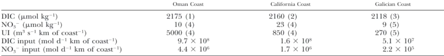
TABLE 2. Comparison in 3 upwelling systems of DIC and NO32concentrations of upwelled water and upwelling index (UI). 15

Sarma (2003); 25 van Geen et al. (2000); 3 5 Borges (unpublished, OMEX II data set); 4 5 Chen et al. (2003); 5 5 A´lvarez-Salgado et al. (2002).

Oman Coast California Coast Galician Coast

DIC (mmol kg21₎

NO32(mmol kg21)

UI (m3_s21_{km of coast}21₎

DIC input (mol d21_{km of coast}21₎

NO32input (mol d21km of coast21)

2175 (1) 10 (4) 5000 (4) 9.73 108 4.43 106 2160 (2) 23 (4) 850 (4) 1.63 108 1.73 106 2118 (3) 9 (5) 270 (5) 5.13 107 2.23 105

filaments that are very efficient structures for the export of organic carbon as DOC and suspended POC to the adjacent deep ocean (A´ lvarez-Salgado et al. 2001, 2003).

Coastal upwelling areas are known to show over-saturation of CO2with respect to atmospheric

equi-librium due to the input of CO2-rich deep waters.

The input of nutrients from upwelling fuels pri-mary production that in turn lowers pCO2 values.

Each of these two processes has an opposing effect on theDpCO2. In the Peruvian and Chilean coastal

upwelling systems, which are known to be among the most productive oceanic areas worldwide, huge oversaturation of CO2 with respect to the

atmo-sphere has been reported with pCO2values up to

1,200 ppm, although low values down to 140 ppm have also been observed in relation to primary pro-duction (Kelley and Hood 1971a; Simpson and Zir-ino 1980; Copin-Monte´gut and Raimbault 1994; Torres et al. 2002, 2003). Other upwelling systems show a lesser range of variation, 100–850 ppm off the California coast (Simpson 1984; van Geen et al. 2000; Friederich et al. 2002), 300–450 ppm off the Mauritanian coast (Copin-Monte´gut and Avril 1995; Lefe`vre et al. 1998; Bakker et al. 1999), and 365–750 ppm off the Oman coast (Ko¨rtzinger et al. 1997; Goyet et al. 1998; Lendt et al. 1999; Sa-bine et al. 2000; Lendt et al. 2003).

The distribution of DIC in upwelling systems is characterized by strong spatial heterogeneity as il-lustrated by high resolution surface mapping off the Portuguese, Californian, and Galician coasts (respectively, Pe´rez et al. 1999; van Geen et al. 2000; Borges and Frankignoulle 2002b). This spa-tial heterogeneity is usually related to topographic features that lead to enhanced upwelling at capes. The width of the continental shelf also determines the ratio of the volume of upwelled water to the volume of water on the shelf, which depends on the ratio between the surface area and the length of the shelf break. This has significant effects on temperature and DIC distributions over the shelf (Borges and Frankignoulle 2002c).

Biogeochemical cycling and air-water CO2fluxes

vary at two distinct temporal scales. At a seasonal scale, the variability is related to the alternation of

upwelling and non-upwelling (or downwelling) seasons. During the upwelling season, the variabil-ity is related to the oscillation between upwelling and upwelling-relaxation events, which have a pe-riodicity ranging from 14 d off the Galician coast (A´ lvarez-Salgado et al. 1993) to 2 d off the Chilean coast (Torres et al. 1999).

Air-water CO2 fluxes have been satisfactorily

in-tegrated in 3 coastal upwelling systems off the Ga-lician, California, and Oman coasts (Table 1). The upwelling system off the Galician coast behaves as a sink for atmospheric CO2, while the other 2

up-welling systems behave as sources for atmospheric CO2. Concentrations of DIC and nitrate (NO32)

and Upwelling Index are significantly higher in the upwelling systems off the Oman and California coasts than the one off the Galician coast (Table 2). Off the Galician coast, at the end of an up-welling-relaxation event (end of the upwelling cy-cle), the surface water is depleted in nutrients and undersaturated with respect to atmospheric CO2

(A´ lvarez-Salgado et al. 2001; Borges and Frankig-noulle 2001, 2002b,c). In the upwelling systems off the Oman and California coasts, the input of DIC and NO32 are so intense (Table 2), that primary

production probably does not deplete surface wa-ters in nutrients and does not induce a significant undersaturation with respect to atmospheric CO2.

Off the Galician coast, large upwelling filaments are characterized by stronger undersaturation with respect to atmospheric CO2 than offshore waters,

affecting significantly the overall budget of air-wa-ter CO2 fluxes in noncoastal (offshore) waters

(Borges and Frankignoulle 2001, 2002b,c). Off the Oman coast, upwelling filaments have been shown to be oversaturated in CO2 with respect to

atmo-spheric CO2(Lendt et al. 1999, 2003). These

struc-tures deserve further research since they actively link the coastal and open oceans and are efficient exporters of organic matter (A´ lvarez-Salgado et al. 2001).

OPENCONTINENTAL SHELVES

Open continental shelves are defined as the coastal zones not comprised in the 7 ecosystems discussed above. Air-water CO2 fluxes have been

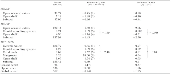
Fig. 4. Budgets of organic carbon (OC) and dissolved inor-ganic carbon (DIC) flows in the North Sea (Thomas et al. 2004b) and the U.S. South Atlantic Bight (Cai et al. 2003). Air-water CO2fluxes are computed as the closing term in the North

Sea budget and are computed from pCO2measurements in the

U.S. South Atlantic Bight budget. Thomas et al. (2004a) provide an estimate of air-water CO2fluxes of21.38 mol C m22yr21for

the North Sea based on pCO2measurements.

satisfactorily integrated in 12 open continental shelves, including a semi-enclosed sea (Baltic Sea) and marginal seas (Table 1). At high latitudes (Ba-rents Sea, Bristol Bay, and Pryzd Bay) and at tem-perate latitudes (Baltic Sea, North Sea, Gulf of Bis-cay, and U.S. Middle Atlantic Bight), open conti-nental shelves behave as sinks for atmospheric CO2

at an annual rate similar to the one reported in the East China Sea. Subtropical and tropical open continental shelves (U.S. South Atlantic Bight, Florida Bay, and Southwest Brazilian coast) behave as significant sources for atmospheric CO2.

Over-saturation with respect to atmospheric CO2 has

also been reported at subtropical latitudes in the Southwest Florida shelf (Clark et al. 2004) and at tropical latitudes in the Eastern Brazil shelf (Ovalle et al. 1999), although the low temporal coverage in these studies does not allow an annual integra-tion of air-water CO2fluxes.

Figure 4 compares DIC and organic carbon areal fluxes in the North Sea and the U.S. South Atlantic Bight. Both systems export carbon (DIC and or-ganic carbon) to the adjacent deep ocean but be-have differently from the point of view of air-water CO2 exchange. River inputs of organic matter are

37 times higher in the U.S. South Atlantic Bight than in the North Sea. Total inputs of organic mat-ter (rivers, Baltic Sea, and English Channel) are 7 times smaller in the North Sea than in the U.S. South Atlantic Bight. The net export of carbon (DIC and organic carbon) to the Atlantic Ocean is about 5 times higher in the North Sea (22.96 mol

C m22 _yr21_{) than in the U.S. South Atlantic Bight}

(4.26 mol C m22 _yr21_{). On one hand the North}

Sea receives less organic carbon from external sources and on the other hand exports more effi-ciently carbon to the deep adjacent ocean. Note that according to the budgets in Fig. 4 both systems are net heterotrophic but organic carbon con-sumption is almost 4 times more intense in the U.S. South Atlantic Bight (3.71 mol C m22 _yr21₎

than in the North Sea (0.98 mol C m22 _yr21_).

Another major difference between these two sys-tems is that the North Sea is seasonally stratified while the U.S. South Atlantic Bight is permanently well mixed. In a seasonally stratified system, organ-ic matter produced in the mixed layer can escape across the pycnocline and will be degraded in the bottom water column. The deep bottom water when circulating out of the system exports carbon as DIC to the adjacent deep ocean (this corre-sponds to the ‘‘continental shelf pump’’ as for-mulated by Tsunogai et al. 1999, p. 701). In a per-manently well-mixed system the decoupling of pro-duction and degradation of organic carbon across the water column does not occur, and it will export DIC less efficiently. The CO2 produced by

degra-dation processes will also be to a large extent ven-tilated back to atmosphere over the continental shelf. This could also explain why the English Channel is not a significant sink for atmospheric CO2 unlike other temperate continental shelves

(Table 1), since it is also a permanently well-mixed system. In the English Channel, the amount of CO2

fixed annually by pelagic new production is equiv-alent to the amount of CO2 released by

calcifica-tion from the extensive brittle star populacalcifica-tions (Borges and Frankignoulle 2003).

High latitude continental shelves behave as sig-nificant sinks for atmospheric CO2(Table 1). The

most comprehensive study in these regions is the annual cycle at Pryzd Bay, Antarctica, by Gibson and Trull (1999). In spring, pCO2decreases under

the sea ice due to primary production occurring within or on the bottom of the ice, and can reach record low values of 46 ppm. When the sea ice breaks, surface waters are undersaturated in CO2

and pCO2further decrease due to pelagic primary

production. During the ice free periods, surface waters absorb atmospheric CO2 at very high rates,

on average 211.9 mol C m22 _yr21_{. When sea ice}

forms again, pCO2 increases slowly due to

degra-dation of organic matter and the input of CO2-rich

circumpolar deep water, according to Gibson and Trull (1999). In Brystol Bay, Western Bering Sea, during winter surface waters uncovered by sea ice are oversaturated in CO2 in relation to the

destra-tification of the water column and input to the sur-face of DIC rich deeper waters (Walsh and Dieterle

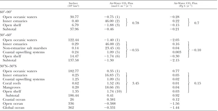
TABLE 3. Air-water CO2flux in open oceanic waters and major coastal ecosystems (excluding inner estuaries and salt marshes), by

latitudinal bands of 308. Surface areas of coastal ecosystems are based on Walsh (1988) and Gattuso et al. (1998a). 1 5 Takahashi et al. (2002) revised climatology for year 1995 (downloaded from http://www.ldeo.columbia.edu/res/pi/CO2/); 25 Average of fluxes in Barents Sea, Bristol Bay, and Pryzd Bay (Table 1); 35 Surface area weighted average of fluxes off the Galician coast (90,000 km2

5 Iberian upwelling system), California coast (La Nin˜a year, 336,000 km2_{), and Oman coast (131,000 km}2_{; Table 1); 45 Surface area}

weighted average of fluxes in Baltic Sea (128,727 km2_{), North Sea (511,540 km}2_{), English Channel (82,600 km}2_{), Gulf of Biscay}

(270,000 km2_{), U.S. Middle Atlantic Bight (63,100 km}2_{), and East China Sea (900,000 km}2_{; Table 1); 55 Average of fluxes in Hog}

Reef, Okinawa Reef, Yonge Reef, and Moorea (Table 1); 65 Average of fluxes in Norman’s Pond, Mooringanga Creek, Saptamikhi Creek, Gaderu Creek, Nagada Creek, and Itaurac¸a Creek (Table 1); 75 Average of fluxes in U.S. South Atlantic Bight, Florida Bay, and Southwest Brazilian coast (Table 1). Fluxes were averaged when different gas transfer velocities were used. Small differences between total and subtotal values and the sum of individual fluxes are related to rounding of numbers.

Surface

(106_km2₎ Air-Water CO_{(mol C m}22_yr2Flux21₎ Air-Water CO_{(Pg C yr}221₎Flux

608–908

Open oceanic waters Open shelf Subtotal 30.77 7.19 37.96 20.75 (1) 21.88 (2) 20.96 20.28 20.16 20.44 308–608

Open oceanic waters 122.44 21.40 (1) 22.06 Coastal upwelling systems

Open shelf 0.24 14.90 1.09 (3) 21.74 (4)    21.69 0.003 20.31    20.308 Subtotal 137.58 21.43 22.36 308N–308S Oceanic waters

Coastal upwelling systems Coral reefs Mangroves Open shelf 182.77 1.25 0.62 0.20 1.60 0.35 (1) 1.09 (3) 1.52 (5) 18.66 (6) 1.74 (7)      2.40 0.77 0.02 0.01 0.04 0.03      0.10 Subtotal 186.44 0.39 0.7 Coastal ocean Open ocean Global ocean 26 336 362 21.170 20.388 20.444 20.37 21.56 21.93

1994). Sea ice coverage in Brystol Bay lasts about 32 d per year compared to 297 d in Pryzd Bay. Sea ice strongly affects air-water CO2exchange as well

as the physical and biogeochemical processes of the underlying water, which in turn affect pCO2.

The duration of sea ice cover should have a critical influence on overall air-water CO2 fluxes; at high

latitudes, it is wise to distinguish between high and low sea ice cover over continental shelves. The ef-fect on air-water CO2 fluxes of sea ice and its

in-teraction with the water column is more complex than the ‘‘seasonal rectification hypothesis’’ first introduced by Yager et al. (1995, p. 4389), as dis-cussed later.

TENTATIVEUP-SCALING AND GLOBAL INTEGRATION To up-scale CO2 fluxes in the coastal ocean, the

fluxes from Table 1 were averaged as explained in the legends of Tables 3 and 4, to characterize 6 ecosystems: coastal upwelling systems, inner estu-aries, non-estuarine salt marshes, coral reefs, man-groves, and open continental shelves. For a given ecosystem the air-water CO2 fluxes were averaged

unless reliable individual surface areas were avail-able and a surface area weighted average was used

instead (details in legends of Tables 3 and 4). Sur-face area estimates for each ecosystem, by latitu-dinal bands of 308, were compiled from Woodwell et al. (1973), Walsh (1988), and Gattuso et al. (1998a). In absence of a global estimate of surface area for outer estuaries and whole estuarine sys-tems, these two ecosystems were not included in the up-scaling. The choice of latitudinal bands is based on the natural delimitation of certain eco-systems, such as coral reefs, mangroves, and salt marshes, and also because in high-latitude conti-nental shelves (608–908), light availability strongly limits primary production (phototrophic) and the presence of extensive sea ice has a significant effect on air-water CO2 fluxes, as discussed above. Two

up-scaling attempts were performed, one exclud-ing inner estuaries and non-estuarine salt marshes (Table 3) and another including inner estuaries and non-estuarine salt marshes (Table 4), since there is considerable uncertainty regarding the surface area estimate of these two ecosystems, as discussed later.

Based on the up-scaling attempt that excludes inner estuaries and salt marshes (Table 3), the coastal ocean behaves as a sink for atmospheric

TABLE 4. Air-water CO2flux in open oceanic waters and major coastal ecosystems (including inner estuaries and salt marshes) by

latitudinal bands of 308. Surface areas of coastal ecosystems are based on Walsh (1988) and Gattuso et al. (1998a). Surface area of inner estuaries was computed using the total surface area of 0.94333 106_km2_{from Woodwell et al. (1973) that was distributed in}

latitudinal bands of 308 based on coastline length from World Vector Shoreline (Soluri and Woodson 1990) implemented in the LOICZ database, downloaded from http://hercules.kgs.ukans.edu/hexacoral/envirodata/main.htm. Surface area of non-estuarine salt marsh surrounding waters is arbitrarily estimated as 50% of the total salt marsh area of 0.27873 106_km2_{from Woodwell et al.}

(1973). 1 5 Takahashi et al. (2002) revised climatology for year 1995 (downloaded from http://www.ldeo.columbia. edu/res/pi/CO2/); 25 Surface area weighted average of fluxes in Randers Fjord (23 km2_{), Elbe (327 km}2_{), Ems (140 km}2_{), Rhine}

(193 km2_{), Thames (215 km}2_{), Scheldt (220 km}2_{), Tamar (19 km}2_{), Loire (110 km}2_{), Gironde (442 km}2_{), Douro (2 km}2_{), Sado (102}

km2_{), and York River (180 km}2_{); 3}5 Average of fluxes in Barents Sea, Bristol Bay, and Pryzd Bay (Table 1); 4 5 Duplin River (Table

1); 55 Surface area weighted average of fluxes off the Galician coast (90,000 km2_{5 Iberian upwelling system), California coast (La}

Nin˜a year, 336,000 km2_{), and Oman coast (131,000 km}2_{; Table 1); 6}5 Surface area weight average of fluxes in Balic Sea (128,727

km2_{), North Sea (511,540 km}2_{), English Channel (82,600 km}2_{), Gulf of Biscay (270,000 km}2_{), U.S. Middle Atlantic Bight (63,100}

km2_{), and East China Sea (900,000 km}2_{; Table 1); 7}5 Average of fluxes in Satilla River, Hooghly, Godavari, and Mandovi-Zuari (Table

1); 85 Average of fluxes in Hog Reef, Okinawa Reef, Yonge Reef, and Moorea (Table 1); 9 5 Average of fluxes in Norman’s Pond, Mooringanga Creek, Saptamikhi Creek, Gaderu Creek, Nagada Creek, and Itaurac¸a Creek (Table 1); 105 Average of fluxes in U.S. South Atlantic Bight, Florida Bay, and Southwest Brazilian coast (Table 1). Fluxes were averaged when different gas transfer velocities were used. Small differences between total and subtotal values and the sum of individual fluxes are related to rounding of numbers.

Surface

(106_km2₎ Air-Water CO_{(mol C m}22_yr2Flux21₎ Air-Water CO_{(Pg C yr}221₎Flux

608–908

Open oceanic waters 30.77 20.75 (1) 20.28 Inner estuaries Open shelf 0.40 6.79 46.00 (2) 21.88 (3)    0.78 0.22 20.15    0.7 Subtotal 37.96 20.46 20.21 308–608

Open oceanic waters 122.44 21.40 (1) 22.05 Inner estuaries

Non-estuarine salt marshes Coastal upwelling systems Open shelf 0.29 0.14 0.24 14.47 46.00 (2) 23.45 (4) 1.09 (5) 21.74 (6)      20.55 0.16 0.04 0.003 20.30      20.10 Subtotal 137.58 21.30 22.15 308N–308S

Open oceanic waters 182.77 0.35 (1) 0.77 Inner estuaries

Coastal upwelling systems Coral reefs Mangroves Open shelf 0.25 1.25 0.62 0.20 1.35 16.83 (7) 1.09 (5) 1.52 (8) 18.66 (9) 1.74 (10) 









CO2 (21.17 mol C m22 yr21) and the uptake of

atmospheric CO2by the global ocean increases by

24% (21.93 versus 21.56 Pg C yr21_{). The inclusion}

of the coastal ocean increases the estimates of CO2

uptake by the global ocean by 57% for high lati-tude areas (20.44 versus 20.28 Pg C yr21_{) and by}

15% for temperate latitude areas (22.36 versus 22.06 Pg C yr21_{). At subtropical and tropical}

lati-tudes, the contribution from the coastal ocean in-creases the CO2emission from the global ocean by

13% (0.87 versus 0.77 Pg C yr21_{). At subtropical}

and tropical latitudes, the coastal environment that has the largest contribution to the increase of the CO2 emission from the global ocean is mangrove

surrounding waters (5%), followed by open con-tinental shelves (4%), coastal upwelling systems (3%), and coral reefs (1%). Coastal upwelling

sys-tems have a moderate effect on air-water CO2

bud-get of the coastal ocean and a low effect on the budget of the global ocean. Using the air-water CO2flux from the Galician coast (22.0 mol C m22

yr21_{) leads to an increase of the uptake of CO} 2

from the coastal ocean of 14% (20.42 Pg C yr21₎

but only of 3% from the global ocean (21.98 Pg C yr21_{). Using the air-water CO}

2flux from the

Cal-ifornia coast (2.2 mol C m22 _yr21_{) leads to a}

de-crease of the uptake of CO2from the coastal ocean

of 6% (20.35 Pg C yr21_{) but only 1% from the}

global ocean (21.90 Pg C yr21_).

Based on the up-scaling attempt that includes inner estuaries and non-estuarine salt marshes (Ta-ble 4), the coastal ocean behaves as a source for atmospheric CO2 (0.38 mol C m22 yr21) and the

decreases by 12% (21.44 versus 21.56 Pg C yr21_).

The emission of CO2 from non-estuarine salt

marshes (0.04 Pg C yr21_{) is equivalent to the one}

from mangrove surrounding waters but remains modest compared to the emission of CO2from

in-ner estuaries globally (0.43 Pg C yr21_{) or at}

tem-perate latitudes exclusively (0.16 Pg C yr21_{). At}

high and subtropical and tropical latitudes, the coastal ocean behaves as a source for atmospheric CO2but at temperate latitudes, it still behaves as a

moderate sink for atmospheric CO2. At temperate

latitudes, the inclusion of coastal ocean increases the CO2 uptake by the global ocean by 5%

com-pared to 15% when estuaries and non-estuarine salt marshes are excluded (Table 3). At high lati-tudes, the inclusion of coastal ocean decreases the CO2 uptake by the global ocean by 25%. At

sub-tropical and sub-tropical latitudes, the contribution from the coastal ocean increases by 20% the CO2

emission from the global ocean, compared to 13% when estuaries and non-estuarine salt marshes are excluded (Table 3).

CONCLUDINGREMARKS

At this point, the major pieces lacking from the jigsaw puzzle will be identified and can be separat-ed into the detail of the up-scaling procseparat-edure (i.e., further classification within each given ecosystem) and lack of characterization (in space and time) of air-water CO2 fluxes. Future changes of air-water

CO2fluxes in the coastal ocean will also be briefly

discussed.

DETAIL OF THEUP-SCALINGPROCEDURE Due to the relative paucity of available data, the up-scaling of air-water CO2 fluxes in the coastal

ocean was attempted based on a limited classifica-tion of ecosystems and simple surface area esti-mates divided in 308 latitudinal bands. The classi-fication of continental shelves can be further de-tailed, based on the geometry (broad shelves: .100 km and narrow shelves: ,50 km), the river discharge of sediments (high: .108 tons yr21 _and

low: ,106 tons yr21_{), and freshwater discharge}

(Wollast and Mackenzie 1989; Mackenzie 1991; Wollast 1998).

In inner and outer estuaries and open continen-tal shelves, presence or absence of a seasonal or permanent stratification seems to be a critical fac-tor controlling air-water CO2 fluxes. In stratified

systems the organic carbon produced by primary production can escape the surface layer across the pycnocline and the CO2produced by degradation

processes in the bottom waters is not readily avail-able for exchange with the atmosphere. Stratified (microtidal) estuaries are lower sources of atmo-spheric CO2 than well-mixed (macrotidal)

estuar-ies. In permanently well-mixed systems, the decou-pling between production and degradation of or-ganic matter can occur in time but does not occur across the water column. These systems are sources of CO2to the atmosphere or neutral, based on the

data available to date. Shallow continental shelves are usually well-mixed systems and in these systems the overall effect of benthic calcification can be stronger than in deeper continental shelves, as il-lustrated by the neutral air-water CO2fluxes in the

English Channel. In coral reefs, the data compiled by Suzuki and Kawatha (2003) suggest that fring-ing reefs are lower sources or even sinks for at-mospheric CO2compared to barrier and atoll reefs

systems. In coral reefs, residence time and volume of the water mass and calcification rates are the main controlling factors of air-water CO2fluxes. In

mangrove and salt marsh surrounding waters, there are not enough data to determine the factors responsible for the intersite variability of air-water CO2fluxes, but the combination of residence time

and volume of the water mass and organic carbon delivery to the creeks seems to be the most likely candidate.

In the future, up-scaling of CO2 fluxes in the

coastal ocean besides obvious latitudinal partition-ing (high latitude, temperate, and subtropical-tropical) could be further detailed at least accord-ing to: macrotidal versus microtidal for estuaries; shallow versus deep and well-mixed versus (season-ally or permanently) stratified for temperate and subtropical-tropical open continental shelves; high versus low sea ice annual coverage for high latitude open continental shelves; high versus low Upwell-ing Index for upwellUpwell-ing systems; and frUpwell-ingUpwell-ing ver-sus barrier-atoll for coral reefs.

Figure 5 shows that about 60% of freshwater dis-charge and an equivalent fraction of riverine total

organic carbon (TOC 5 DOC 1 POC) delivery

occur at subtropical and tropical latitudes. Coun-terintuitively, less than 12% of the CO2 emission

from inner estuaries occurs at these latitudes and the highest emission of CO2 occurs at high

lati-tudes, although characterized by the lowest fresh-water discharge and riverine TOC delivery. There is also a counterintuitive anticorrelation between the latitudinal distribution of freshwater discharge and the surface area of inner estuaries. Although no data of air-water CO2 fluxes are available in

high latitude inner estuaries, the values used at temperate and subtropical and tropical latitudes can be considered as robust. Discrepancies re-vealed in Fig. 5 are probably due to the uncertainty on the estimate of the surface area of inner estu-aries and on its partitioning by latitudinal bands, rather than on the air-water CO2areal fluxes. The

Fig. 5. Latitudinal distribution of the freshwater discharge (based on Dai and Trenberth [2002]), of the inner estuaries surface area, river total organic carbon (TOC) inputs (based on Ludwig et al. [1996]), and CO2emission from inner estuaries

(Table 4). Surface area of inner estuaries was computed using the total surface area of 0.94333 106_km2_{from Woodwell et al.}

(1973) that was distributed in latitudinal bands of 308 based on coastline length from World Vector Shoreline (Soluri and

←

Woodson 1990) implemented in the LOICZ database, down-loaded from http://hercules.kgs.ukans.edu/hexacoral/enviro-data/main.htm.

Woodwell et al. (1973, p. 225) has been widely used in literature although these authors caution their own estimate: ‘‘It would be surprising if esti-mates derived in this way were accurate within 6 50%.’’ They estimated a ratio of inner estuary sur-face area to coast length for the U.S. that they ex-trapolated to the worldwide coastline.

Abril and Borges (2004) estimated that the glob-al CO2 emission from inner estuaries due to

deg-radation of allochthonous riverine POC is around 0.09 Pg C yr21_{, assuming that about 50% of riverine}

POC is remineralized during estuarine transit (based on Abril et al. 2002) and using the global POC riverine input given by Ludwig et al. (1996). The fact that the present estimate is almost 5 times higher (0.43 Pg C yr21_{, Table 4) would confirm the}

idea that the inner estuary surface area given by Woodwell et al. (1973) is overestimated. At least four arguments can be raised that bring both es-timates closer together. Based on more recent data Richey (2004) provides a higher value (0.50 versus 0.18 PgC yr21_{) of allochthonous riverine POC}

ex-port to the coastal zone than Ludwig et al. (1996). This would bring the estimate of CO2emission due

to the degradation of allochthonous riverine POC to 0.25 Pg C yr21_{. The assumption of a 50%}

remin-eralization of riverine POC of Abril et al. (2002) is based on the study of 9 European estuaries. Keil et al. (1997) estimated that in the Amazon delta more than 70% of riverine POC is remineralized during estuarine transit. This would bring the es-timate of CO2 emission due to the degradation of

allochthonous riverine POC to 0.35 Pg C yr21_.

There is increasing evidence that lateral inputs of TOC and DIC in both polluted and pristine estu-aries are highly significant compared to the river-ine carbon inputs (Cai and Wang 1998; Cai et al. 1999, 2000; Neubauer and Anderson 2003; Gazeau et al. 2004a), although much less well constrained at the global scale. The contribution of the venti-lation of river DIC to the overall emission of CO2

from inner estuaries seems highly variable from one estuary to another but also highly significant, ranging from 10% to 50% in the Scheldt inner estuary and Randers fjord, respectively. This last point clearly highlights the importance of the con-cept that coastal ecosystems are not closed and constitute a continuum exchanging in both direc-tions of carbon and nutrients with adjacent sys-tems. The estimated overall emission of CO2from

sur-Fig. 6. Percentage of surface area of continental shelves by latitudinal bands in the Northern and Southern Hemisphere (based on data from Walsh [1988]).

face area of Woodwell et al. (1973) could be a rea-sonable first-order estimate. The latitudinal parti-tioning of the emission from inner estuaries is most probably flawed based on the counterintui-tive trends shown in Fig. 5.

The estimation of the role of estuaries in the budget of CO2 exchanges in the coastal ocean is

further complicated by the contribution from out-er estuaries that is highly significant as discussed above for the Scheldt and Amazon whole estuarine systems. No global surface area estimate is available for outer estuaries for which there is also a lack of air-water CO2 flux estimates. The actual

computa-tion of the air-water CO2 fluxes is not

straightfor-ward in whole estuarine systems since the gas trans-fer velocity can be assumed to be mainly depen-dant on wind stress in outer estuaries and the con-tribution of tidal currents to water turbulence will increase upstream at least in macrotidal inner es-tuaries (Borges et al. 2004b).

In the present tentative up-scaling, the inclusion of inner estuaries leads to the reversal of the di-rection of air-water CO2fluxes in the coastal ocean

and it seems critical to evaluate the surface area of inner and outer estuaries and its latitudinal parti-tioning with some accuracy. To achieve this, geo-graphical information systems as those developed in the framework of LOICZ or sophisticated water mass analysis and classification schemes of satellite images (e.g., Oliver et al. 2004) seem to be prom-ising approaches.

The relative contribution of the CO2 emission

from salt marsh surrounding waters compared to the one from inner estuaries is small in the present up-scaling but would increase if the surface area of inner estuaries would be revised to a lower value. Note that the surface area of salt marsh surround-ing waters is also derived from Woodwell et al. (1973) and should also be used with caution. The estimation of the surface area of salt marsh and mangrove surrounding waters is very approximate and also requires a re-evaluation in the future. It was assumed that the surface area of surrounding waters is equivalent to the one of the correspond-ing intertidal zone covered by these habitats. Their overall role in the exchange of CO2 with the

at-mosphere is further complicated by the fact that emerged intertidal sediments also emit CO2to the

atmosphere at high rates (e.g., in the mangrove forests of Gazi Bay, Kenya, ranging between 4 and 165 mol C m22_yr21_{[Middelburg et al. 1996] and}

in the salt marshes of Oyster Landing, U.S. South Atlantic Bight, ranging between 19 to 27 mol C m22_yr21 _{[Morris and Whiting 1986]).}

Although there are not enough data to partition with confidence the up-scaling of air-water CO2

fluxes in the coastal ocean into the two

Hemi-spheres (since most data are available in the North-ern Hemisphere, see Fig. 1), the relative distribu-tion of the surface area of continental shelves clearly shows that the coastal ocean will have a much more marked effect on the global CO2

flux-es in the Northern Hemisphere (Fig. 6). The rel-ative contribution of the Northern Hemisphere to the uptake of atmospheric CO2and its partitioning

into oceanic and terrestrial biospheres is the sub-ject of a long lived debate initiated by the work of Tans et al. (1990). These authors attributed to the terrestrial biosphere a missing sink of CO₂between 22.0 and 23.0 Pg C yr21 _{at temperate latitudes}

required to balance the global CO2 budget

con-strained with the North-South gradient of atmo-spheric CO2. In the budget of Tans et al. (1990),

the upper bound of the open ocean CO2sink was

estimated to be20.9 Pg C yr21_{but at present time}

it has been re-evaluated at 21.6 Pg C yr21

(Taka-hashi et al. 2002). The missing sink of CO2at

tem-perate latitudes to constrain the North–South gra-dient of atmospheric CO2 can be roughly

re-eval-uated between21.3 and 22.3 Pg C yr21_{. The}

high-er bound of the sink for atmosphhigh-eric CO2 in the

coastal ocean at temperate latitudes is 20.3 Pg C yr21 _{(Table 3) and probably mostly located in the}

Northern Hemisphere (roughly 20.26 Pg C yr21

based on Fig. 6), and is not negligible in relation to the missing CO2 sink (contribution between

23% and 13%).

Besides coastal and open oceanic waters, signif-icant CO₂exchanges are also associated with lakes (global CO2 emission of 0.1 Pg C yr21, Cole et al.

1994), rivers (global CO2emission of 0.3 Pg C yr21,

Cole and Caraco 2001), and freshwater wetlands (CO2 emission of 0.5 Pg C yr21 from central

Am-azon wetlands alone, Richey et al. 2002). In the context of a global evaluation of CO2fluxes,

aquat-ic systems should be envisaged together since they constitute a continuum where carbon from the ter-restrial biosphere and the atmosphere cascades.