The Oxford Handbook of Productivity Analysis
E. Grifell-Tatjé, C. A. K. Lovell and R. C. Sickles, Editors.
Chapter 17th
Productivity and Welfare Performance in the Public Sector
*Mathieu Lefebvre, Université de Strasbourg Sergio Perelman, Université de Liège
Pierre Pestieau, Université de Liège and CORE, UCL.
Abstract
In times of budgetary difficulties it is not surprising to see the performance of the public sector questioned. What is surprising is that what is meant by it, and how it is measured, does not seem to matter to either the critics or the advocates of the public sector. The purpose of this chapter is to suggest a definition and a way to measure the performance of the public sector or rather of its main components. Our approach is explicitly rooted in the principles of welfare and production economics. We will proceed in three stages. First of all we present what we call the "performance approach" to the public sector. This concept rests on the principal-agent relation that links a principal, i.e., the public authority, and an agent, i.e., the person in charge of the public sector unit, and on the definition of performance as the extent to which the agent fulfils the objectives assigned to him by the principal. Performance is then measured by using the notion of productive efficiency and of "best practice" frontier technique. We then move to the issue of measuring the productivity of some canonical components of the public sector (railways transportation, waste collection, secondary education and health care). We survey some typical studies of productive efficiency and emphasize the important idea of disentangling conceptual and data problems. This raises the important question that given the available data, does it make sense to assess and measure the productivity of such public sector activities? In the third stage we try to assess the performance of the overall public sector. We argue that for such a level of aggregation one should restrict the performance analysis to the outcomes and not relate it to the resources involved. As an illustration we then turn to an evaluation of the performance of the European welfare states and its evolution over time, using frontier techniques. The results confirm that countries with lowest performance grew faster but this is not sufficient to confirm a path towards convergence.
* The authors are grateful to the editors and to Humberto Brea for insightful comments and suggestions on previous versions of this chapter. Sergio Perelman acknowledges financial support from the Belgian Fund for Scientific Research - FNRS (FRFC 14603726 - “Beyond incentive regulation”).
17.1 Introduction
In both developed and less developed countries, one can speak of a crisis of the public sector. The main charge is that it is costly for what it delivers; costly at the revenue level (tax distortion, compliance cost) and at the spending level (more could be produced with less); costly or at least costlier than would be the private sector. Even though this particular charge is rarely supported by hard evidence it has to be taken seriously because of its impact on both policy makers and public opinion. The purpose of this chapter is to address the question of whether we can measure the productivity of the public sector, a question that is very general and terribly ambitious. Consequently we will narrow it down by dealing with it in two stages. In the first stage we consider the public sector as a set of production units that use a number of resources within a particular institutional and geographical setting and produce a number of outputs, both quantitative and qualitative. Those outputs are related to the objectives that have been assigned to the production unit by the principal authority in charge, i.e., the government. If the principal were a private firm, the objective assigned to the manager would be simply to maximize profit. However with public firms or sectors there are multiple objectives.
For example, in the case of health care or education, maximizing the number of QALYS (years of life adjusted for quality) or the aggregate amount of human capital respectively, is not sufficient. Equity considerations are also among the objectives of health and education policy. Within such setting the productivity is going to be defined in terms of productive efficiency, and to measure it, we will use the efficiency frontier technique. Admittedly productive efficiency is just a part of an overall efficiency analysis. It has two advantages: it can be measured, and its achievement is a necessary condition for any other type of efficiency. Its main drawback however is that it is based on a comparison among a number of rather similar production units from which a best practice frontier is constructed. Such a comparative approach leads to relative measures, and its quality depends on the quality of the observation units. There exists a large number of efficiency studies concerned with the public sector. Some focus exclusively on public units; others compare public and private units. We will present a small sample of these studies, whose characteristic is that even the best of them do not use the ideal data due to lack of availability. Particularly qualitative evidence is missing for both outcomes and inputs. Under the hard reality that data are insufficient, if not missing, the question is whether or not some productivity studies make sense.
Whereas in the above studies there is a quite good relation between the outputs and the inputs, when we move up to an aggregate level the link is not clear anymore. For example, public spending in health is not related to the quality of health, for at least two reasons: health depends more on factors such as the living habits or the climate than on spending and spending can be higher where it is needed, namely in areas of poor health. For this reason, when dealing with the public sector as a whole we prefer to restrict our analysis to the quality of outcomes and not to the more or less efficient relation between resources used and outcomes. The problem becomes one of aggregation of outcome indicators. In this chapter, we illustrate our point by evaluating the performance of the European welfare states. We use the DEA technique with a unitary input. This technique gives different weights to each
indicator and each decision unit, here each national welfare state. So doing, we expect that the weight given to a partial indicator and to a specific country reflects the importance that this country gives to this indicator. We thus meet the concern of political scientists that different welfare states can have different priorities.1 This approach, which has been labelled benefit of
the doubt by Cherchye et al. (2007a), was proposed by Melyn and Moesen (1991) and Lovell et al. (1995) as an alternative way to measure countries’ macroeconomic performance and used, among others, by Cherchye et al (2004) and Coelli et al. (2010) to measure the performance of European welfare states.2
Accordingly, in the last section of this chapter we update Coelli et al (2010) using five normalized outcomes indicators – which concern poverty, inequality, unemployment, education and health – for the 28 European Union members states, 15 historical members (EU15) and 13 newcomers (EU13), over the period 2005-2012. We compare the results obtained using identical weights, an average social protection index (SPI), and the DEA benefit of the doubt approach, either without imposing constraints on outcomes weights, or by imposing 10% minimum weights on each of them. As expected, some countries’ rankings vary dramatically depending of the weighting approach (SPI, unconstrained or constrained DEA). Nevertheless when we analyse the dynamics of performance over the 2005 to 2012 period a test of the mean reversion hypothesis confirms that countries with lower performance grew faster. Unfortunately this is a necessary but not a sufficient condition for convergence and the tests we perform indicate that convergence in welfare states performance among the EU28 members is not yet achieved.
To sum up the spirit of this chapter, we believe that the study of the productivity of the public sector should comprise two parts: an evaluation of the productive efficiency of its components and an assessment of its achievements as a whole. The next two sections are devoted to these two parts.
17.2 Efficiency measures of public firms and services
There is a long tradition of efficiency measurement in the public sector and a wide number of studies report the results of productivity comparisons concerning public firms and services. As we will illustrate here with some examples – railways transportation, waste collection by municipalities, secondary education and health care – there exists a gap between the ideal data needed for such assessments and the data used in the economic literature. On the one hand, there are the restrictions imposed by data availability – mainly sample size limitations, small number of units and short periods – which constrain the number of dimensions that could be taken into account simultaneously, independently of the methodology used. On the other hand, it is difficult to identify and to measure accurately the final outcomes, those which
1 See, e.g., Esping-Andersen (1990).
2 The benefit of the doubt approach has been also applied to other fields, e.g. to measure the performance of European
internal market dynamics (Cherchye et al. (2007b)); farms sustainability (Reig-Martínez et al (2011)); citizen satisfaction with police services (Verschelde and Rogge (2012)); citizens wellbeing (Reig-Martínez (2013)); or in the case of undesirable outputs (Zanella et al (2015).
justify the public nature of the firm or the activity including quality dimensions. Reliable qualitative information on outputs is often missing. Also relevant quality features of inputs as well as information on the environmental conditions in which these firms operate are often neglected. We are interested in these deviations from the ideal data. Our goal is to present a list of variables for a few examples, that in our view would be the ideal dimensions to consider, assuming no data restriction. We rely on Pestieau (2009) for the description of ideal data.
Furthermore, the objectives assigned by governments and regulatory agencies to public firms and public services are multidimensional. Other than technical efficiency and allocative (price) efficiency, they often include macroeconomic (growth and employment) and distributive (equity) targets.3 Most of the literature covered focuses only on efficiency without
considering prices, costs minimization or profit maximization, nor macroeconomic and distributive targets. There are however some rare exceptions.
17.2.1 Railways transportation
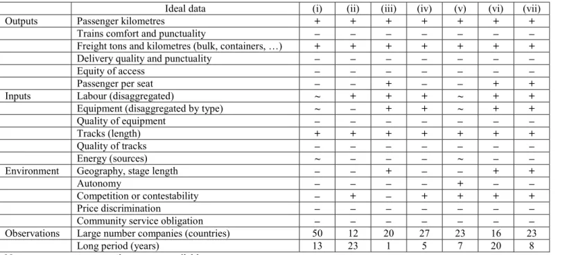
Our first example is productive efficiency in public railways transportation. The list of variables presented in Table 17.1 assumes no data availability restrictions. Besides output quantities, number of passengers, journey length and tons of freight transported, we include quality indicators: comfort, reliability of delivery and punctuality. Equity of access is also a key dimension: How accessible is railways transportation to different categories of the population, e.g. distinguished by income and location? Which are the types of inputs used in production: i) staff skills and experience; ii) type and quality of equipment; iii) length and quality of tracks; and iv) different sources of energy? In our view, all these dimensions are relevant and would be considered in a benchmark study.
Furthermore, given the nature of the activity, railways companies operate, by definition, in different geographical areas and national institutional environments. Therefore, other than geographical characteristics, e.g. average stage length and population density, it is crucial to have information on railways sector regulations, e.g. autonomy of management, degree of competition, market contestability. Last but not least, we want to know if they are subject to community service obligations and, perhaps, to constraints regarding price discrimination. Over the last decade, several studies were published on European railways productivity. The aim of most of them was to analyze the effects of the European Commission railways deregulation policy, launched in the early nineties. The main objectives of this reform, as summarized by Friebel et al. (2008), were: (a) to unbundle infrastructure from operations; (b) to create independent regulatory institutions and (c) to open access to the railways markets for competitors. Most European countries slowly introduced these reforms and this gave the opportunity to make efficiency comparisons among them, particularly between vertically integrated and still unbundled companies. With the exception of Farsi et al. (2005), which study the productivity of Swiss regional and local railways networks, and Yu and Lin (2008),
3 As stated by Pestieau and Tulkens (1993), even if these objectives are not always completely compatible, there
which compare European railways productivity in 2002, the studies surveyed in Table 17.1 use panel data to draw conclusions pertaining to the effect of the ongoing deregulation process in the EU. In Table 17.1, as well as in the following tables in this section, we use different signs to indicate that a particular dimension – output, input or environment (non-discretionary) variable – is taken into account (“+ = yes”) or not (“– = no“) according to the ideal data, or either if it is considered but not completely (“~ = more or less”).
INSERT TABLE 17.1
Undoubtedly among the potential consequences of the reform, transportation quality and equity of access are key issues, as well as quality of track and of equipment. However, as we show in Table 17.1, none of these dimensions was taken into consideration in the reviewed studies. Farsi et al. (2005) estimate cost efficiency of 50 subsidized railways in Switzerland using alternative parametric approaches. They show the importance of taking into account firms’ heterogeneity in Stochastic Frontier Analysis (SFA). They rely on duality theory and, for this purpose, use input prices instead of quantities (“~” in Table 17.1). Friebel et al. (2008) estimate technical efficiency and productivity growth of 13 European railways using a Linear Structural Relations (LISREL) model. As for the other studies of European national railways presented here, data for countries with unbundled systems was previously aggregated across all railways companies (infrastructure and operations) operating within a country. Yu and Lin (2008) use a multi-activity Data Envelopment Analysis (DEA) approach to compute technical efficiency and effectiveness of 20 European railways in 2002, including seven Eastern European railway.4 Growitsch and Wetzel (2009) estimate economies of scope, for integrated
vs. unbundled railways companies, using DEA and data of 27 European Railways over the period 2000-2004. Asmild et al. (2009) address also the effect of reforms on European railways efficiency using a multi-directional DEA approach. This approach allows them to compute, separately, staff and material purchases (OPEX less staff expenditures) cost efficiency and to compare them across Europe taking into account competition, contestability and the companies’ autonomy. Cantos et al. (2010) compute technical efficiency, technical change and productivity growth using DEA, while Cantos et al. (2012) compare DEA and SFA results. In both cases the authors test the influence of vertical integration vs. unbundled railways controlling simultaneously for population density.
Summing up, none of the studies surveyed here considers outputs and inputs quality dimensions. Moreover, none of them control for the potential role on railways outcomes, eventually played, by two institutional particular features: price discrimination and community service obligations.
17.2.2 Waste collection
In most countries around the world, waste collection is a public service whose responsibility falls on local authorities, municipalities in the majority of cases. In Table 17.2 we present the ideal data that should be considered in the model. On the output side, we expect to find,
4 The authors make in this way the distinction between railways “efficiency”, measured with outputs corresponding to the
supplied capacity (seats-km and tons-km supplied) and “effectiveness”, with outputs corresponding to effective demand (seats-km and tons-km transported).
garbage collected in tons and by type, the service coverage and the quality, the scores reflecting environment protection (like the percentage of waste recycling), air and water quality, and depletion of non-renewable resources.5 On the input side, the choice of variables
will depend on the unit characteristics. For instance, for the firms that manage waste collection at the municipal level, it would be possible to use information on physical inputs, like labour and equipment, but only if they correspond exactly to the same area for which the outputs are observed. Given the increasing organisational complexity of waste collection, that implies high specialisation and economies of scale, most municipalities outsource these activities. In this case, the input is represented by one variable, the total cost paid by the municipality for waste collection and treatment, which includes direct cost plus outsourcing. Finally, as for the other analysed public services environmental (non-discretionary) factors must be taken into consideration. The distance to landfill and the collection frequency are two other variables in relation with the geography and population density. Also the age structure and the socio-demographic characteristics of the population must be considered, especially when they vary dramatically across municipalities. Moreover, as mentioned before, outsourcing is unavoidable in most cases for municipalities, and is therefore potentially a way to improve the services offered and to benefit from economies of scale. In the same line of reasoning, the way municipalities price waste collection – weight-based, pay-per-bag, poll tax, …– may influence waste production behaviour of the population.
INSERT TABLE 17.2
In Table 17.2 we survey the dimensions considered by authors in some recent studies selected here for illustration purposes. Worthington and Dollery (2001) measure cost efficiency in domestic waste management among New South Wales municipalities using DEA. Their study has the particularity to work with a large sample and to take into account the recycling rate and municipalities’ geographic and demographic dimensions. García-Sánchez (2008) analysed the efficiency of waste collection in Spanish municipalities with more than 50,000 inhabitants which “… are obliged by law to provide the same solid waste services…” (p. 329). The author computes DEA efficiencies using output and inputs quantities and in a second stage tests the effect of non-discretionary factors, including socio-economic dimensions. Marques and Simões (2009) study the effect of incentive regulation on the efficiency of 29 Portuguese waste management operators in 2005. For this purpose, they first compute a two-output (tons collected and tons recycled) two-input (OPEX and CAPEX) DEA model and, in a second stage, analyse the effect of non-discretionary variables, among them the institutional framework (private vs. public and regulatory schemes). It is interesting to note that the authors report a detailed list of performance indicators, which includes quality of service and environmental sustainability. This list is published every year by the regulatory agency (Institute for the Regulation of Water and Solid Waste, IRAR), as part of a so-called “sunshine” regulation. This kind of information is also part of our ideal data. Unfortunately, Marques and Simöes decided to not include them in the analysis, because “…they are defined by legislation with high sanctions for non-compliance with laws and regulations” (p. 193).
Finally, we include in Table 17.2 three recent studies in which the authors study the effect of waste-reducing policies on waste collection and treatment costs of near three-hundred municipalities in Flanders, Belgium. Particularly, these studies make the distinction among outputs according to waste types: green, packaging, bulky, residual and EPR (extended producer responsibility: batteries, car tires, electrical equipment …). De Jaeger et al. (2011) compute a DEA model with total costs as input and then test the effect of demographic and socio-economic non-discretionary variables, controlling for institutional differences such as weight based pricing, cooperation agreement and outsourcing. Rogge and De Jaeger (2012) use slightly similar updated information but rely on a shared input DEA model which allows computing partial cost-efficiency for different waste types. Finally, De Jaeger and Rogge (2013) compute Malmquist productivity indexes for the period 1998 to 2008. The results show that, contrary to expectations, weight-based pricing municipalities did not perform worse in terms of cost efficiency than with pay-per-bag system.
In summary, recent productivity studies on waste collection consider garbage composition, total costs paid by municipalities and most non-discretionary dimensions. They generally fail to include quality of service and environment sustainability indicators.
17.2.3 Secondary education
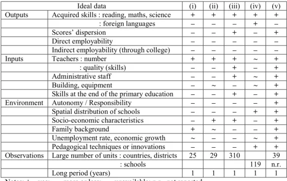
In Table 17.3, we illustrate what would be the ideal data to study education productivity and, for this purpose, we choose secondary education. What are the objectives of the government (national or local) on educational matters? It is reasonable to expect high skills in reading comprehension, as well as in mathematics, sciences and foreign languages. Given that students come from different backgrounds, we do not only need indicators on average scores but also scores’ dispersion. Moreover, the capacity to find employment or access to higher education, matters too.
On the input side there are two possible views: physical or financial. The physical inputs are number and quality of teachers, administrative staff, the building and other educational materials. Alternatively one can look at overall public spending. In such case there are two steps embodied: the first step from the financial spending to physical inputs, where inputs prices matter, and the second step from inputs to outputs. Therefore, using financial spending as input implies, as a potential shortcut, a source of bias in productivity comparisons. Finally, the skills acquired by students at the end of primary school would be ideally included as an input of secondary education.
The environmental variables which must be considered vary with the level of aggregation: country, district or school. In a within country comparison one has the advantage of dealing with the same institutional and cultural setting but a number of other dimensions matter, above all the socio-economic environment: income inequality, unemployment, population size and density. Also the family background and the peer group characteristics are important. In a between-country comparison, it is expected to include institutional variables like: political decentralization (schools autonomy), competition of private schools, educational system (mobility of students, selectivity, pedagogical techniques …).
In the literature we find best practice comparisons between countries, between districts within a country and between schools, either within or across countries or districts. Most international comparative studies rely on data collected at student level either by the OECD Program for International Student Assessment (PISA) or by the International Association for the Evaluation of Educational Achievement (IEA) Trends in International Mathematics and Science Study (TIMSS).
In Table 17.3 we present the list of outputs, inputs and environmental variables used in a selected number of studies. Afonso and St Aubyn (2006a) use PISA data aggregated by country in international comparisons. As expected, given the small number of observations (25 countries), the number of variables taken into account is reduced to a strict minimum. Sutherland et al. (2009) compare education efficiency in OECD countries using PISA but relying on disaggregated data at the school level. This allows them to take into account simultaneously the family and socio-economic background, as well as a proxy of capital (computer availability). Both studies also report the results of cost-efficiency comparisons at the national level using information on educational expenditures. Besides the difficulty to estimate accurately the real cost of education, there is evidence from Hanushek (1997) survey of near 400 studies on the US education that “there is not a strong or consistent relationship between student performance and school resources, at least after variations in family inputs are taken into account” (p. 141). This is not surprising given the objectives of welfare states concerning education, which are not merely to maximize the average scores and expected earnings, but the overall distribution (equity). This is the reason why family background and socioeconomic environment play a key role in many studies.
INSERT TABLE 17.3
In Table 17.3 we report the variables used by Grosskopf et al. (1997) to compare the productivity of 310 educational districts in Texas. For this purpose the authors use a parametric indirect distance function approach which considers the scores obtained by students in previous levels of education. As inputs, other than school teachers, they consider three staff categories: administration, support and teacher aides. Haelermans and De Witte (2012) compare 119 schools productivity in the Netherlands looking for the impact of educational innovations. They use a nonparametric conditional (order-m) approach which allows for controlling schools heterogeneity, mainly localization. Unfortunately, given data limitations, school inputs are represented by a unique variable: expenses per student. Finally, Wößmann (2003) used probably the largest international data set available, 39 countries and more than 260.000 students who participated in the TIMMS study in 1994-95. The author estimates an education production function using parametric models, ordinary and weighted least squares to identify the main drivers of education performances. We choose this study as an illustration that ideal data is not an unattainable goal, at least for input and environmental variables. In addition to the ones indicated in Table 17.3, Wößmann (2003) includes several variables controlling for teachers’ influence, school responsibility, parents’ role and students’ incentives.
To summarize, all these studies use data on students’ acquired skills and on the number of teachers, but only in two cases, Grosskopf et al. (1997) and Wößmann (2003), one uses information on output inequality (scores’ dispersion), on teachers’ quality and, even more importantly, on students’ skills at the end of the primary school. Moreover, none of the studies in Table 17.3 considers information on the courses followed by the students after high school, the degree of employability or the pursuit of higher education. Such information is obviously difficult to obtain.
17.2.4 Health care
Assuming perfect data availability, we would like to use data reflecting how the patients expected lifetime and health status increase as a consequence of health care use. At the same time, as indicated in Table 17.4, we would like to consider as output the quality of the care delivered. We are not only interested by the efficiency of medical treatment but also by the way this is delivered. Using individual data it would be possible to compute for these variables average values and inequality indicators (distribution).
On the input side, we would consider the number and the quality of physicians, nurses and hospitals, and how these inputs are distributed among the population and geographical terms. Furthermore, total social spending is a potential substitute of physical and qualitative input variables when the information on inputs is sparse or not reliable.
Environmental factors play a crucial role on health care delivered. Other than the age structure of the population, individual lifestyle factors like smoking, poor diet or lack of physical activity matter. Institutions may also have an important role, e.g. the share of prevention in total care expenditures, the importance of the private health sector and the private health insurance, co-payment by patients, etc. Our expectation is that most of the necessary information might be available, even if not in the exact desired form.
Before turning to a few recent cross-country comparative studies, the first study in Table 17.4, Crémieux et al. (1999), deals with Canadian provinces and is not interested by the measurement of productivity, but by the estimation of an average health care production function. The reason we choose this study is that it illustrates very well that collecting ideal data is not an impossible task, at least for the ten Canadian provinces over the period 1978-1992. The authors use information on health care outputs and inputs together with detailed information on population socio-economic composition and on individuals’ behaviour.
INSERT TABLE 17.4
The other studies presented in Table 17.4 deal with cross-country health care data compiled either by the World Health Organisation (WHO) or by the Organization for Economic Co-operation and Development (OECD). Evans et al. (2000) and Tandon et al. (2001) used as health outputs, respectively, the “disability-adjusted life expectancy” (DALE) measure and a composite measure, which considers five dimensions: DALE, health inequality, responsiveness-level, responsiveness-distribution and fair-financing.6 Both studies deal with
WHO data on 191 countries over the 1993-1997 period and DEA methodology. Two inputs are considered: total health expenditure (public plus private) and average educational attainment in the adult population.
The results of these studies, also reported in The World Health Report 2000 (WHO, 2000), generated some debate and other studies were undertaken using the same WHO data file.7
Two of them are included in Table 17.4. First, Greene (2004) estimates stochastic frontiers using alternative approaches, which take into account countries’ heterogeneity and several environmental (non-discretionary) variables such as income inequality, population density and the percentage of health care paid by the government. Second, Lauer et al. (2004) estimated health care systems performance assuming five different outputs, in fact, those included in the composite output measure used by Tandon et al. (2001) but taken separately. The particularity of the DEA approach used by Lauer et al. (2004) is that, rather than considering the five different outputs separately, it assumes an identical (equal to 1.0) input for all countries. It is the so called benefit of the doubt model introduced by Melyn and Moesen (1991) and Lovell et al. (1995), which we adopt in the following section to measure the performance of the welfare state in European Union countries.
Finally, we include in Table 17.4 three other studies, Färe et al. (1997), Afonso and St Aubyn (2006b) and Joumard et al. (2008), which used OECD data on health care for industrialized countries. Färe et al. (1997) compute Malmquist productivity indexes for 10 countries over the period 1974-1989. The outcome of health care is represented by life expectancy of women at age 40 and the reciprocal of the infant mortality rate. Inputs are the number of physicians and care beds per capita. Afonso and St Aubyn (2006b) computed technical efficiency of 25 countries in 2002 using the free disposal hull (FDH) approach. In their study the health care production function is specified with two outputs, infant survival rate and life expectancy, and three inputs, the number of doctors, nurses and beds, respectively. In a recent study, Spinks and Hollingsworth (2009) recognized that “the OECD health dataset provides one of the best cross-country sources of comparative data available”, however they also underline pitfalls in this data, mainly “the lack of an objective measure of quality of life”, like additional quality-adjusted life years (QALYs), and a “measure of country-based environmental status”. A study by Joumard et al. (2008) partially answered these criticisms by including on the input side a lifestyle variable and a proxy for the economic, social and cultural status of the population. Finally, for reasons now discussed, the level of aggregation of some of these studies is highly questionable.
Summing up, none of the comparative studies of public health care systems surveyed here consider all the output-input dimensions of the ideal data. Moreover, when an output or an input is included, in most cases the authors are lead to neglect the qualitative and distributional dimensions, due to lack of data. And even worse there are the environmental (non-discretionary) factors, in particular data on institutional issues like co-payment by patients, or the ratio of curative to preventive care, which are not considered.
17.3 The welfare state performance in the EU
In the previous section we have seen that many components of the public sector can be submitted to the test of best practices and that such exercise is useful to improve its overall efficiency. It is however tempting to try to evaluate the performance of the public sector as a whole, neglecting input constraints. In this section we illustrate it by showing estimates of the performance of European public sectors. We have chosen to limit our analysis to that of the welfare state, which is the most important subset of the public sector. We have two reasons for this: the availability of data and a rather good consensus as to the objectives that the welfare state is supposed to pursue and according to which its performance can be assessed. The objectives of traditional European welfare states are first poverty alleviation and inequality reduction and second protection against life cycle risks such as unemployment, ill health and lack of education. Recently the European Union has adopted new means of governance based on voluntary cooperation that aims at achieving some kind of convergence in the field of social inclusion. This approach is known as the Open Method of Coordination (OMC) and it rests on benchmarking and sharing of best practice. Thanks to the OMC, a variety of comparable and regularly updated indicators have been developed for the appraisal of social protection policies in the twenty-eight European Union country members. The aim is to allow countries to know how well they are performing relative to the other countries.
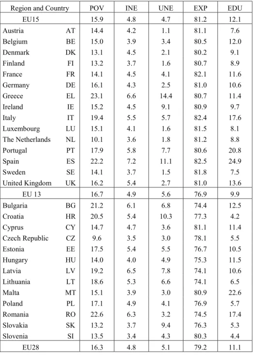
In this section we focus on five of the most commonly used indicators, which concern poverty, inequality, unemployment, education and health. The definitions of the indicators that we use are presented in Table 17.5. The first four indicators, poverty (POV), inequality (INE), unemployment (UNE) and early school leavers (EDU), are such that we want them as low as possible, while life expectancy (EXP) is the only "positive" indicator.8 The five indicators we
are using here cover the most relevant concerns of a modern welfare state and their choice is determined by its objectives.9 They also reflect aspects that people who want to enlarge the
concept of GDP to better measure social welfare generally take into account, e.g., the classical measurable economic welfare (MEW) developed by Nordhaus and Tobin (1972), and more recently revisited by Stiglitz et al. (2009) and by the OECD (2014).
INSERT TABLE 17.5
These indicators for the 28 European Union member states are available for the 8 year period from 2005 to 2012. Table 17.6 lists the values for the year 2012.10 As shown in Table 17.6
countries are not good or bad in all respects and it is difficult to make global comparison. We are unable to confidently say that a country is doing better than another country unless all five
8 The data are provided by the EU member states within the OMC (see Eurostat database on Population and Social
Conditions, http://ec.europa.eu/eurostat/web/income-and-living-conditions/data). They deal with key dimensions of individual well-being; and are comparable across countries. It is difficult to find better data for the purpose at hand. This being said, we realize that they can be perfected. There is some discontinuity in the series of inequality and poverty indicators. In addition, one could argue that life expectancy in good health is likely to be preferred to life expectancy at birth or an absolute measure of poverty might be better than a relative measure that is too closely related to income inequality. But for the time being, these alternatives do not exist.
9 The five indicators belong to the series of ten indicators chosen by EU members as representative of economic and social
policy targets fixed by the 2000 Lisbon Agenda, the so-called “Laeken indicators” (Council of the European Union, 2001).
10 Coelli et al. (2010) study the performance of social protection in the EU15 over the period 1995-2006. This section can be
indicators in the country are better than (or equal to) those in the other country. This is possible in a few cases, e.g. Austria is doing better than Bulgaria in the five indicators, but it is not the norm. To address this issue we wish to obtain a performance index of the welfare state, so that we can say which country is actually doing better than the others. This is of course not without making choices regarding the methods we shall use and this is the purpose of this section.
INSERT TABLE 17.6
To obtain one performance index that summarizes the information contained in the five given indicators we have to make methodological choices. First the indicators should be converted so that they are comparable; this is the case of the indicators where a higher value is bad. Second, we should decide of how we aggregate the five indicators retained here. Should we use a linear aggregation function (as for the Human Development Index, HDI) or should we rely on more sophisticated techniques as presented above? If we use a simple average of the five indicators, they need to be scaled so that they are measured with the same unit. Finally, we could allocate weights to each of the five indicators in the aggregation process. Should these weights vary across indicators? Furthermore should these weights vary across countries? And, could they take extreme values, like zero?
In what follows we address these questions by presenting successively three indexes of the performance of the European welfare states. Starting from a simple linear aggregation index, we then present two estimations based on best practice frontier techniques. On the one hand, the original DEA approach which allows for free choice of output weights, with the only condition of non-negativity and, on the other hand, a DEA which allows for imposing minimum constraints on the weights assigned to each output.11
At this point it is important to stress that if we assume that these five indicators as well as the aggregate indicator measure the actual outcomes of the welfare state (what we call its performance), it would be interesting to also measure the true contribution of social protection to that performance and hence to evaluate to what extent the welfare state, with its financial and regulatory means, gets close to the best practice frontier. We argue that this exercise, which in production theory amounts to the measurement of productive efficiency, is highly questionable at this level of aggregation.
Henceforth when we compare the performance of the welfare state across countries we do not intend to explain it by social spending. We realize that many factors may explain differences in performance. First the welfare state is not restricted to spending but includes also a battery of regulatory measures (minimum wage, tax expenditures, safety rules, etc…) that contribute to protect people against lifetime risks and to alleviate poverty. Second contextual factors such as family structure, culture and climate, may explain educational or health outcomes as much as anything else. This is why we limit our exercise to what we call performance assessment and argue against any efficiency/productivity analysis.
11 For example, see O’Donnell’s chapter in this volume for details of the DEA method. See also Cherchye et al. (2004) who
17.3.1 Scaling
The first task is to normalize the five variables in order to make them comparable but also to include them in a simple linear aggregation index. Indeed the five indicators listed in Table 17.5 are measured in different units. In the original Human Development Report (HDR, 1990), three composite indicators (health, education and income) are used to derive a Human Development Index (HDI). The authors suggest scaling these indicators so that they lie between 0 and 1, where the bounds are set to reflect minimum and maximum targets. Thus we propose a simple scaling so that the n-th indicator (e.g., life expectancy) of the i-th country should be scaled using:
, (1)
so that for each indicator the highest score is 1 and the lowest is 0. For “negative” indicators, such as unemployment, where “more is bad”, one alternatively uses:
(2)
so that the country with the lowest rate of unemployment will receive a score of 1 and the one with the highest rate of unemployment will receive 0. This is not the only way of scaling indicators and the results may be dependent of the chosen method. Coelli et al. (2010) compare several scaling methods and show that the results are impacted, although marginally, by the approach adopted.
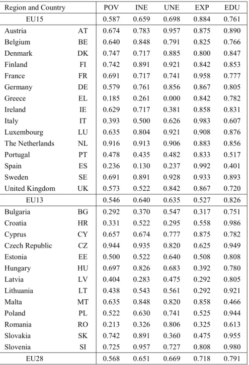
Table 17.7 shows the five normalized indicators for our sample of 28 countries in 2012. We purposely distinguish between the 15 historical members of the EU (hereafter EU15) and the 13 more recent newcomers (EU13). For normalization purposes we take the minimum and the maximum values out of the all sample period 2005-2012 such that these extreme values can be observed at different time. Near all the extreme (maximum and minimum) values of the five indicators correspond to the years before 2012.
INSERT TABLE 17.7
17.3.2 Measuring performance
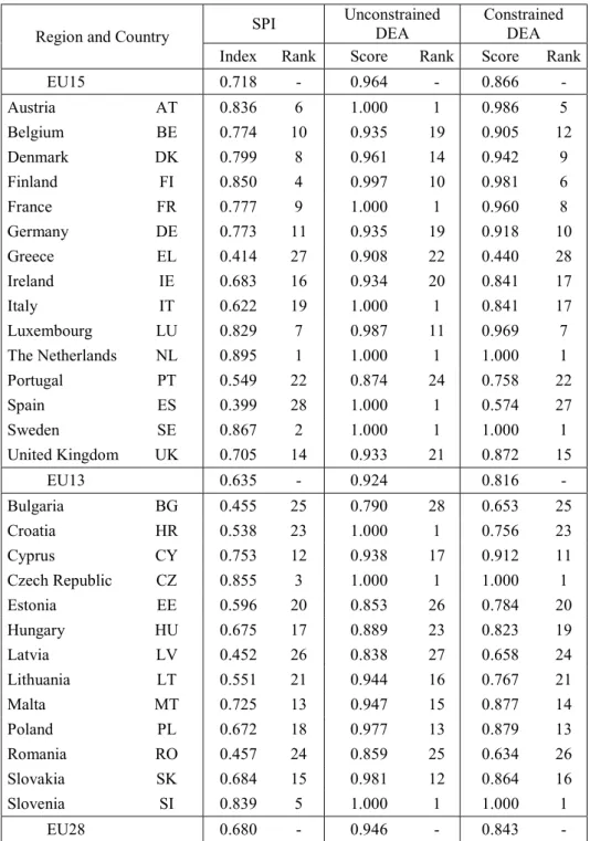
On the basis of the five scaled indicators, we want to obtain an overall assessment of the welfare state performance. One option is to follow the HDI method exposed above and calculate the raw arithmetic average of the five indicators. We call it the social protection
* min{ } max{ } min{ } ni nk k ni nk nk k k x x x x x * max{ } max{ } min{ } nk ni k ni nk k nk k x x x x x
index: . Table 17.8 reports the indicators as well as the rank of each country in
2012. As it appears, we have at the top the Nordic countries, plus Austria, the Netherlands and Luxembourg. But we also have new entrants countries (EU13) doing quite well like Slovenia or Czech Republic which are at the top. At the bottom, we find Bulgaria, Greece, Latvia, Romania and Spain.
However this summation of partial indicators is quite arbitrary and does not completely respond to the estimation problems we raised earlier. In particular, there is no reason to grant each indicator the same weight. In fact weights could change across indicators and across countries to account for the fact that different countries have different priorities. Indeed some countries may give more weight to employment than to income equality and other countries may give more weight to poverty than to education. One possible solution to this problem is to use the DEA approach. As seen in the previous section DEA is traditionally used to measure the technical efficiency scores of firms. In the case of the production of social protection by a welfare state, we could conceptualise a production process where each country is a “firm” which uses government resources to produce social outputs such as reduced unemployment and longer life expectancies. We do not follow this path but we will assume that each country has one “government” and further one unit of input, and that it produces the five outputs discussed above.
As indicated in the introductory section, this approach is known in the literature as the benefit of the doubt weighting approach. It was often applied to compare the performance of production units – countries, public services, farms, … – as an alternative composite indicator of performance, the one which takes in consideration idiosyncratic units’ behaviour. More concretely, the DEA benefit of the doubt scores reported on Table 17.8, called here unconstrained DEA, are computed under the assumption that each unit freely chooses the most favourable share weights bundle.
A number of observations can be made from the unconstrained DEA scores and rankings reported on Table 17.8.12 First, we note that approximately 30% of the sample receives a DEA
efficiency score of one (indicating that they are fully efficient). This is not unusual in a DEA analysis where the number of dimensions (variables) is large relative to the number of observations. Second, the average DEA score is 0.946 versus the mean SPI score of 0.680. The DEA scores tend to be higher because the unlimited freedom to choose outcomes’ weight compared with SPI uniform weights assumption. Third, the DEA rankings are “broadly similar” to the SPI rankings. However a few countries do experience dramatic changes, such as Italy, Spain and Croatia which are ranked 19, 28 and 23 respectively under SPI but are found to be fully efficient in the DEA results.
12 In order to perform DEA computations we rescaled the five output indicators between 0.1 and 1.0, instead of 0.0 to 1.0.
The main reason is to avoid zero outputs and then allow constrained share weights DEA computations. The DEA efficiency scores reported here do not take into account slacks; therefore they are invariant to this simple units measurement change in scaling, as it has been proved by Lovell and Pastor (1995).
5 1 * 5 1 n ni i x SPIINSERT TABLE 17.8
There are two primary reasons why we observe differences between the rankings in DEA versus the SPI. First, the SPI allocates an equal weight of 1/5 to each indicator while in the DEA method the weights used can vary across the five indicators. They are determined by the slope of the production possibility frontier that is constructed using the linear programming methods. Second, the implicit weights (or shadow prices) in DEA can also vary from country to country because the slope of the frontier can differ for different output (indicator) mixes. We use the shadow price information from the dual DEA linear programming to obtain the implicit weights assigned to each country indicator. These weights and their means are given on Table 17.9. The first thing we note is that the poverty (POV) and inequality (INE) indicators are given, in average for the whole sample EU28, a fairly small weight, while life expectancy (EXP) and education (EDU) indicators are given a weight much larger than 0.3. These results suggest that the uniform weights of 0.2 (used in the SPI) understate the effort needed to improve health and education outcomes versus reducing inequality and poverty. Nevertheless, when we observe more in details the results for EU15 and EU13, we remark that huge differences appear. Several EU15 members, mainly Italy, Portugal and Spain, assign the highest weight (higher than 0.9) to life expectancy, while several EU13 countries, among them Croatia, Latvia and Lithuania, do the same with education. In each case, these countries take advantage of their outstanding performances in these respective domains (see Tables 17.6 and 17.7).
INSERT TABLE 17.9
Summing up, SPI and unconstrained DEA correspond to two aggregation techniques. Many attempts have then been made in the DEA literature to improve the implicit weighting procedure. They mainly consist in the inclusion of additional weight restrictions on the DEA linear program or, in other words, in restricting implicit rates of substitution (transformation) between outputs. Allen et al. (1997) and Cherchye et al. (2007a) summarized the approaches proposed in the literature, which in most cases rely on the role of experts’ value judgements.13
An interesting illustration of the use of experts’ judgements in a benefit of the doubt DEA setting is the study on health performances of 191 World Health Organisation countries members by Lauer et al. (2004), mentioned above. In the case analysed here, the performance of EU welfare states, unfortunately we do not have access to experts’ value judgements. Hence we decided to adopt the same weight restriction for our five indicators. We now present the DEA results obtained assuming equal minimum weights thresholds. For illustration purposes, we choose a minimum threshold of 0.10 for each one the five outcomes indicators which by construction implies a maximum weight threshold of 0.60 for each of them.
13 There are however some exceptions. For instance, Anderson et al. (2011) introduce a benefit of the doubt index which by
construction will be bounded in both sides with only relying on two assumptions: non-decreasing and quasi-concave with respect to indicators; also Reig-Martínez et al. (2011) and Reig-Martínez (2013) apply a benefit of the doubt index in combination with a Multi Criteria Decision Method (DEA-MCDM) which allows building a full rank of all observations in the sample, included the most efficient.
The results reported in the last columns of Table 17.8 were obtained imposing absolute weight restrictions.14 That is, instead of imposing restrictions on shadow prices, these are
imposed on indicators’ virtual proportions (Wong and Beasley (1990)). More concretely, each output is assumed to have a weight not lower than 0.10, as indicated before.
Clearly the DEA scores obtained under weight restrictions are either equal or lower than those obtained under unconstrained DEA (Pedraja-Chaparro et al. (1997)). On Table 17.8 we observe that four countries, Czech Republic, The Netherlands, Slovenia and Sweden, keep their position on the frontier in 2012, while several others suffer of sharp performance drop, accompanied in some cases by dramatic loss in rank position, like Croatia, Greece, Italy or Spain. Finally, many other countries, including Belgium, Cyprus, Denmark and Germany, improved dramatically their rank even if their performance diminished in absolute terms. Average constrained DEA scores (0.843) are, as expected, located between unconstrained DEA (0.946) and SPI (0.680) scores, but closer to the former. On the contrary, individual countries’ performances are highly correlated between constrained DEA and SPI (0.982 Spearman correlation) when compared with correlation between constrained and unconstrained DEA (0.606 Spearman correlation).
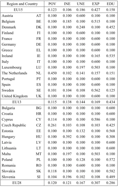
A look at the detailed weights obtained under constrained DEA in Table 17.10 shows that for a majority of countries and indicators the minimum weight constraints (0.10) are binding in 2012. Moreover, for more than half of countries one of the indicators reaches the maximum potential weight, 0.60, while the four others receive the minimum weight threshold. If we compare the average weights for the EU15, EU13 and EU28 in Tables 17.9 and 17.10, it appears that in most cases the weights computed under unconstrained and constrained DEA are very close, with life expectancy (EXP) highly weighted by former European Union members (EU15) and education (EDU) by the new EU13 entrants. The only exceptions are the POV (at-risk-of-poverty-rate) indicator, whose weight doubles from 0.060 to 0.120 for EU28 and the EXP indicator, whose weight increases from 0.089 to 0.169 for EU13.
INSERT TABLE 17.10
17.3.3 Welfare performance dynamics and convergence
The data we used in the previous sections is available for EU27 since 2005, thus it is interesting to see whether we observe specific trends and particularly convergence towards welfare state performance among the EU countries, the aim of the OMC strategy. For this purpose, we compute year by year performance indexes – SPI and constrained DEA – and their rate of change using the 2005-2012 normalized indicators. In the case of SPI its rate of change (SPIC) corresponds to performance growth, while for the DEA score it represents changes in distances to the frontier (relative performance) over time. In order to estimate performance growth in the case of the DEA indicator, we compute Malmquist decomposable indexes of performance change (PC), following Cherchye et al (2007b). These indexes are the sum of two components: the change in relative performance, known as the catching-up (CU)
14 For a survey of weight restriction in DEA, see Pedraja-Chaparro et al. (1997), and for a survey on weight restriction in a
component and the change at the frontier level themselves, labelled as the environmental change (EC) component by Cherchye et al (2007b).15
The results by year and by country are reported in Tables 17.11 and 17.12, respectively. It is interesting to note that for both the SPI and the constrained DEA, the average rate of performance change for the EU28 over the whole period, is positive and similar, 0.5% for SPIC and 0.4% for PC. In other words, welfare state performances increased half percentage point every year in average over the 2005-2012 period. Moreover, looking in details at Table 17.11, we observe that SPIC and PC growth rates are in most cases worst after the crisis than before: null and negative growth rates are only observed from 2008-2009 on. Otherwise, several differences appear in the results across methods and between EU15 and EU13 members’ states. For instance, EU15 performed less well than EU13 members, in average, both under SPIC (-0.1% vs. 1.2%) and constrained DEA (0.2% vs. 0.6%). When we analyse the components of performance change, catching-up (CU) and environmental change (EC), a clear case appears for EU13 with a positive catching-up growth rate (CU=1.9%) with a simultaneous decrease at the frontier level, EC=-1.3% in average for the whole period.
INSERT TABLE 17.11
To be complete, Table 17.12 reports the results by country. For several countries both methodologies give similar results, for some of them positive SPIC and PC, e.g. Belgium, Portugal and Slovenia, for other negative, e.g. Denmark and Bulgaria. Only France presents results of opposite sign, with a negative performance rate of change under SPI, but positive under constrained DEA. Overall the correlation between both indicators is high (0.964 Pearson correlation).
INSERT TABLE 17.12
To test convergence in performance among EU countries we perform two different tests following Lichtenberg (1994). First, we test the mean-reversion hypothesis, that is the hypothesis that countries with the lowest level of performance at period t-1 growth at a highest rate in period t. For this purpose we run a simple OLS model with the logarithm of the performance score change in time t as dependent variable and as explanatory variable the performance score at time t – 1. This test is a necessary but not a sufficient condition for convergence; therefore we run the test of convergence suggested by Lichtenberg (1994). The results of these tests applied to the performance scores changes (SPIC, PC and CU) are reported in Table 17.13.
Looking first at the results corresponding to the change in performance scores SPIC and PC, we observe that the mean-reversion hypothesis is verified for the two indicators. In both cases the coefficient β associated with lagged performance has a negative and statistically significant value. Moreover β takes a similar absolute value, -0.037 and -0.042 for the SPI and
15 This component represents the technological progress in the productivity measurement literature (Färe et al. (1994)). In the
performance measurement framework, Cherchye et al. (2007b) postulate that this component “reflects a more favourable policy environment” (p.770).
constrained DEA, respectively. In other words, countries with the lowest performance score improved their welfare state performance faster.
The test for convergence is straightforward. It is simply based on the ratio 𝑅 (1 + 𝛽)⁄ computed using the OLS estimated parameters.16 As demonstrated by Lichtenberg (1994),
this ratio is equivalent to a test on the ratio of variances between periods, the variance in t-1 over the variance in t. For convergence, the expected result is that this ratio must be higher and significantly different from 1.0. The results reported in Table 17.1 are in both cases slightly higher than 1.0 (SPI=1.005 and constrained DEA=1.036) but none of them significantly different from 1.0.
The second section of Table 17.13 reports the results of mean-reversion hypothesis and convergence test for the catching-up effects (CU) computed under constrained DEA . As for performance growth the mean-reversion hypothesis is verified. The β coefficient is negative and statistically different from zero. The test on ratio 𝑅 (1 + 𝛽)⁄ shows higher values than for PC (1.054), but not sufficiently to validate convergence.
Finally, at the bottom of Table 17.13 are reported the results of a test of unequal variances between performance scores in 2005 and 2012. The ratio, in logarithmic form, indicates a value higher than 1.0 for constrained DEA (1.39). As expected, performance variance declines among the EU28 countries. However, it was not enough to pass the convergence test. In this case, as well as for the ratio of variances corresponding to SPIC (1.01), these values are statistically non-significant.
INSERT TABLE 17.13
Summing up, the results reported here confirm the observations made in Table 17.8. We do not observe convergence in performance among the countries unlike Coelli et al (2010). There are mainly two reasons. The first one comes from the fact that the sample we use is much more limited in terms of time: 2005 to 2012 vs. 1995 to 2006. A second reason to this result is the economic crisis that started in 2007 and had direct consequences on social protection budgets in many countries.
17.3.4 Measuring efficiency with or without inputs
Finally, if we would like to compare these results with those presented in traditional measures of production efficiency of public services or public utilities from Section 17.2, we should gather data on both outputs and inputs to construct a best practice frontier. We showed above that even though it is difficult to meet the ideal data requirement, this approach is very useful and could be used when at least sufficient data are available and there exists an underlying identified technology. For example, measuring the efficiency of railways companies with this
16To perform this test the 𝑅 corresponds to the OLS model with 𝑙𝑜𝑔[𝐷𝐸𝐴(𝑡)] as dependent variable and
approach makes sense. Railways transport people and commodities (hopefully with comfort and punctuality) using a certain number of identifiable inputs.
When dealing with the public sector as a whole and more particularly social protection, we can easily identify its missions: social inclusion in terms of housing, education, health, work and consumption. Yet, it is difficult to relate indicators pertaining to these missions (e.g., our five indicators) to specific inputs. A number of studies use social spending as the only input, but one has to realize that for most indicators of inclusion, social spending explains little. For example, it is well known that, for health and education, factors such as diet and family support are often just as important as public spending. This does not mean that public spending in health and in education is worth nothing; it just means that it is part of a complex process in which other factors play a crucial and complementary role.
Another reason why using social spending as the input of our 5 indicators is not appropriate comes from the fact that social spending as measured by international organisations is not a good measure of real spending. It does not include subsidies and tax breaks awarded to schemes such as mandatory private pensions or health care and it includes taxes paid on social transfers.17
All this does not mean that the financing side of the public sector does not matter. It is always important to make sure that wastes are minimized, but wastes cannot be measured at such an aggregate level. It is difficult to think of a well-defined technology, which “produces” social indicators with given inputs. To evaluate the efficiency slacks of the public sector, it is desirable to analyse micro-components of the welfare states such as schools, hospitals, public agencies, public institution, railways, etc. such as the studies we presented in the previous section. At the macro level, one should stop short of measuring technical inefficiency and restrict oneself to performance ranking.
To use the analogy of a classroom, it makes sense to rank students according to how they perform in a series of exams. Admittedly we can question the quality of tests or the weights used in adding marks from different fields. Yet in general there is little discussion as to the grading of students. At the same time we know that these students may face different “environmental conditions” which can affect their ability to perform. For example, if we have two students ranked number 1 and 2 and if the latter is forced to work at night to help ailing parents or to commute a long way from home, it is possible that he can be considered as more deserving or meritorious than the number 1 whose material and family conditions are ideal. This being said there exists no ranking of students according to merit. The concept of “merit” is indeed too controversial. By the same token, we should not attempt to assess the “merit” of social protection systems or the public sector as a whole.
17.4 Conclusions
The purpose of this chapter was to present some guidelines as to the question of measuring and assessing the performance of the public sector. We believe that such measurement is unavoidable for two reasons. First, people constantly question the role of the public sector as a whole or of its components on the basis of questionable indicators. Second, a good measure can induce governments or public firms that are not performing to get closer to the best practice frontier.
We start with the issue of whether or not we have to limit ourselves to a simple performance comparison or we can conduct an efficiency study. We argue that efficiency evaluations can be conducted for components of the public sector when sufficient data are available and there exists a production technology link between resources used and outcomes achieved. When dealing with the overall welfare state or large aggregates such as the health or the education sector we deliberately restrict ourselves to performance comparisons, that is, comparisons based only on the outcomes of these sectors. The reason is simple: in those instances, the link between public spending and outcomes is not clear and does not reveal a clear-cut production technology. More concretely, key factors that can affect performance are missing. For example, diet can impact health and family can influence education and yet it is difficult to quantify the roles of diet and of family.
We present an overview of recent productive efficiency studies in four areas: railways, waste collection, schools and hospitals. For each of these areas we contrast what we call the ideal set of data with the one that is actually used by researchers. No surprisingly the qualitative data are consistently missing. This weakens the recommendations that can be drawn from these studies and should induce public authorities to further invest in qualitative data collection. We then turn to the assessment of the performance of 28 European Union country members. The fact that even with a synthetic measure of performance the Nordic countries lead the pack is not surprising. It is neither surprising to see that some Mediterranean countries, Greece and Portugal, and most new entrants (EU13) are not doing well. It is interesting to see that with such a comprehensive concept Anglo-Saxon welfare states, Ireland and UK, do as well as the Continental welfare states such as Belgium and Germany, and that Czech Republic and Slovenia are among the best performers.
Finally we turned to the convergence issue. Contrary to Coelli et al. (2010), we did not find a clear-cut process of convergence. This can be explained by the fact that here we deal with EU28 and not just EU15 and that the period is not only much shorter but also includes crisis years. It will be interesting to redo this exercise in several years when a longer time series is available.
References
Adema, W., Fron, P. and M. Ladaique (2011), “Is the European welfare state really more expensive? : Indicators on social spending, 1980-2012; and a Manual to the OECD Social Expenditure Database (SOCX)”, OECD Social, Employment and Migration Working Papers, No. 124, OECD Publishing (doi: 10.1787/5kg2d2d4pbf0-en).
Afonso A. and M. St Aubyn (2006a), “Cross-country efficiency of secondary education provision: A semi-parametric analysis with non-discretionary inputs”, Economic Modeling, 23(3), 476-491.
Afonso A. and M. St Aubyn (2006b), “Non-parametric approaches to education and health efficiency in OECD Countries”, Journal of Applied Economics, 8,2, 227-246.
Allen, R., A.D. Athanassopoulos, R.G. Dyson and E. Thanassoulis (1997), “Weight Restrictions and Value Judgements in DEA: Evolution, Development and Future Directions”, Annals of Operations Research, 73, 13-34.
Anderson, G., Crawford, I. and A. Leicester (2011), “Welfare rankings from multivariate data, a nonparametric approach”, Journal of Public Economics, 95, 247-252.
Asmild, M., Holvad, T., Hougaard, J. L. and D. Kronborg (2009), “Railway reforms: Do they influence operating efficiency?”, Transportation 36, 617-638.
Cantos, P., Pastor, J. M. and L. Serrano (2010), “Vertical and horizontal separation in the European railway sector and its effects on productivity”, Journal of Transport Economics and Policy, 44, 139-160.
Cantos, P., Pastor, J. M. and L. Serrano (2012), “Evaluating European railway deregulation using different approaches”, Transport Policy, 24, 67-72.
Cherchye, L., Moesen, W. and T. Van Puyenbroeck (2004), “Legitimely diverse, yet comparable: on synthesizing social inclusion performance in the EU”, Journal of Common Market Studies, 42(5), 919-955.
Cherchye, L., Moesen, W., Rogge, N. and T. Van Puyenbroeck (2007a), “An introduction to Benefit of the Doubt composite indicators”, Social Indicators Research, 82, 111-145.
Cherchye, L., Lovell, C. A. K., Moesen, W., and T. Van Puyenbroeck (2007b), “One market, one number? A composite indicator assessment of EU internal market dynamics”, European Economic Review, 51, 749-779.
Coelli, T.J., Mathieu Lefebvre and Pierre Pestieau, (2010) "On the convergence of social protection performance in the European Union," CESIfo Economic studies, 56(2), 300-322. Council of the European Union (2001), “Report on indicators in the field of poverty and social exclusion”,
(http://www.consilium.europa.eu/uedocs/cms_data/docs/pressdata/en/misc/DOC.68841.pdf). Crémieux, P.Y., Ouellette P. and C. Pilon (1999), “Health care spending as determinants of health otucomes”, Health Economics, 8, 627-639.
De Jaeger, S., Eyckmans, J., Rogge, N. and T. Van Puyembroeck (2011), “Wasteful waste-reducing policies? The impact of waste reduction policy instruments on collection and processing costs of municipal solid waste”, Waste Management, 31, 1429-1440.
De Jaeger, S. and J., Rogge (2013), “Waste pricing policies and cost-efficiency in municipal waste services: the case of Flanders”, Waste Management & Research, 31(7), 751–758.
Emery, A., Davies A., Griffiths, A. and K. Williams (2007), “Environmental and economic modelling: A case study of municipal solid waste management scenarios in Wales”, Resources Conservation & Recycling, 49, 244-263.
Esping-Andersen, G. (1990), The Three Worlds of Welfare Capitalism, Princeton, N. J., Princeton University Press.
Eurostat (2014), Database on Population and Social Conditions, (http://ec.europa.eu/eurostat/data/database).
Evans D., Tandon A., Murray C. J. L. and A. Lauer (2000), “The comparative efficiency of National Health Systems in producing health: An analysis of 191 countries”, WHO GPE Discussion Paper Series 29, Geneva (http://www.who.int/healthinfo/paper29.pdf).
Färe, R., Grosskopf, S., Norris, M. and Z. Zhang (1994), “Productivity growth, technical progress and efficiency change in industrialized countries”, American Economic Review, 84, 66-83.
Färe, R., Grosskopf, S., Lindgren, B. and J. P. Poullier (1997), “Productivity growth on health-care delivery”, Medical Care, 35, 4, 354-366.
Farsi, M., Filippini, M. and W. Greene (2005), “Efficiency measurement in network industries: Application to the Swiss railways companies”, Journal of Regulatory Economics, 28(1), 69-90.
Friebel, G., Ivaldi, M. and C. Vibes (2008), “Railway (de)regulation: A European efficiency comparison, Economica”, 77, 77-91.
Gakidou, E., Murray, C. J .L. and J. Frenk (2000), “Measuring preferences on health system performance assessment”, WHO EIP/GPE Discussion Paper Series 20, Geneva (http://www.who.int/healthinfo/paper20.pdf).
García-Sánchez, I. M. (2008), “The performance of Spanish solid waste collection”, Waste Management & Research, 26, 327-336.
Greene (2004), “Distinguishing between heterogeneity and inefficiency: stochastic frontier analysis of the World Health Organization’s panel data on national health care systems”, Health Economics, 13, 959–980.
Grosskopf, S., Hayes, K. J., Taylor, L. L. and W. L. Weber (1997), “Budget-constrained frontier measures of fiscal equality and efficiency in schooling”, Review of Economics and Statistics, 79(1), 116-124.
Grotwisch, C. and H. Wetzel (2009), “Testing for economies of scope in European railways. An efficiency analysis”, Journal of Transport Economics and Policy, 43(1), 1-24.
Haelermans, C. and K. De Witte (2012), “The role of innovations in secondary shool performance – Evidence from a conditional efficiency model”, European Journal of Operational Research, 223, 2, 541-549.