HAL Id: hal-01500585
https://hal.archives-ouvertes.fr/hal-01500585
Submitted on 21 Jun 2017
HAL is a multi-disciplinary open access
archive for the deposit and dissemination of
sci-entific research documents, whether they are
pub-lished or not. The documents may come from
teaching and research institutions in France or
abroad, or from public or private research centers.
L’archive ouverte pluridisciplinaire HAL, est
destinée au dépôt et à la diffusion de documents
scientifiques de niveau recherche, publiés ou non,
émanant des établissements d’enseignement et de
recherche français ou étrangers, des laboratoires
publics ou privés.
Tomography
Myriam Servières, Nicolas Normand, Jean-Pierre Guédon
To cite this version:
Myriam Servières, Nicolas Normand, Jean-Pierre Guédon. A Mojette Transform Approach to Discrete
Medical Tomography. First Malaysia-France Regional Workshop on Image Processing in Vision System
and Multimedia Communication, Apr 2003, Kuching, Malaysia. pp.1–11. �hal-01500585�
A MOJETTE TRANSFORM APPROACH
TO DISCRETE MEDICAL TOMOGRAPHY
Myriam SERVIERES , Nicolas NORMAND , Jeanpierre GUEDON
IRCCyN-IVC CNRS UMR 9567,
École polytechnique Université de Nantes, France
Rue Christian Pauc, La chantrerie, BP 60601, Nantes, F44036, France
{myriam.servieres; nicolas.normand ; jean-pierre.guedon }@polytech.univ-nantes.fr
I Introduction
The Radon transform has encountered many trials to change its ill-posed nature into a well-posed
problem. Recovering an initial bulk of data (medical, astronomy, seismology, quality control, etc.) from a set of
projections has been an important vector of progress during the last fifty years. However, for a specific
implementation the tomographist has to study three different kinds of problems. The first one is the geometry of
acquisition (dimension of the initial data, number and angles of projections, spatial position of the bins) and the
way to represent it in an adequate manner on the computer. This leads to the expression of a specific discrete
Radon operator which (generally) has lost its properties of linearity and shift-invariance; at most, it would tends
to the continuous operator if you had an infinite number of projections, pixels, bins. Second, the acquisition
device has to be modeled and all kind of new non-linearities have to be taken into account (blur of the detector,
attenuation process, mismatch of the projection of the center of rotation, etc.). Third, noise appears. Then things
are going from bad to worse. Effectively, if the first step has not been made correctly, the discrepancy between
the continuous and discrete (implemented) inverse Radon transform will be responsible for a significant amount
of errors into the pixel reconstructed value. Even if this error is low (say 5%), since the radiations that you are
giving to a patient (respectively receiving from stars) are low, the contrast sensibility on the image where the
medical doctor (resp. the astronomer) want to perform a given task of tumor (resp. double stars) detection of is
low. Thus, the first step in this overall process is to perform the computer imagery as better than you can since it
The goal of this paper is to put some foundations on the way of obtaining a discrete Radon transform that
keep the linearity and shift-invariance properties of the continuous version, and to derive new algorithms
allowing to adapt the discrete version to the acquisition system. In section 2, the Mojette transform is presented
as the only way to obtain an exact discrete Radon transform. This transform has been derived and used for
different kind of applications ranging from image analysis, watermarking, packet transport, since 1995 by
Guédon and Normand. As explained in section 3, the way of reconstructing 2D weighted shape from discrete
projections will not be directly useful when noise and acquisition degradations will be part of the game. Section
4 allows for merging FBP, the most traditional approach to medical tomographic reconstruction with the Mojette
transform. In section 5, the application of this approach to 3D-PET specific geometry is given and the tools
inherited from the Mojette transform presented.
II From Radon to Mojette transform
2.1 DISCRETE RADON TRANSFORM
A judicious way to obtain a discrete exact Radon operator proceeds as follows. In 2D, the continuous
Radon transform is described by :
proj(t, θ)=R f(x,y)=
⌡
⌠
-∞ +∞⌡
⌠
-∞ +∞f(x,y) δ(t + xsinθ – ycosθ) dxdy. (1) However, an infinite set of projections is needed to represent the continuous function f( x,y). The
functional projection of f(x,y) onto a spline space {ϕ(x-k), k∈Z} leads to an interpolation equation :
fϕ (x,y) = +∞
Σ
k=-∞ +∞Σ
l=-∞ f (k,l).ϕ(x-k).ϕ(y-l). (2)When the discrete pixel grid f(k,l) is considered in the tomographic problem, the function f(x,y) in Eq. (1)
is replaced by fϕ (x,y) of Eq. (2). This leads (after inverting discrete and continuous sum signs) to a definition of the continuous projection from a discrete image and the spline interpolating function.
When ϕ is taken as ϕ(x) = δ(x). Eq. (1) becomes
projδ(t,θ)= +∞
Σ
k=-∞ +∞Σ
l=-∞ f (k,l) δ(t + k.sinθ-l.cosθ). (3)Since functions cosθ and sinθ are giving pure real values, (k.sinθ – l.cosθ) is of elliptical form and the
only possibility to equally sample variable t is to use angles of the form tanθ = q
p . In such a case, cosθ = p h and
sinθ = q
h , and by sampling the t axis with b=t.h, the definition of the Dirac-Mojette transform definition
finally is: Mδf(k,l)=proj(b,p,q)= +∞
Σ
k=-∞ +∞Σ
l=-∞ f(k,l)∆(b + qk – pl), (4) where ∆ (b) = 1 if b=00 if b ? 0 is the discrete Kronecker symbol.
2.2 BASIC 2D MOJETTE PROPERTIES
Eq. (4) resumes the definition of a discrete projection operator but with strange properties compared to
the usual ways of obtaining discrete Radon versions. First, linearity and shift-invariance is kept : this is not true
for most discrete Radon transforms! This major point comes from the fact that angular and projection samplings
are realized in an adequate manner. Generally, for medical devices the discrete version is obtained by taking into
account the discrete pixel size and the same sampling size in the projection but with an infinite number of angles.
Using a finite number of angles removes the linear and shift-invariance properties.
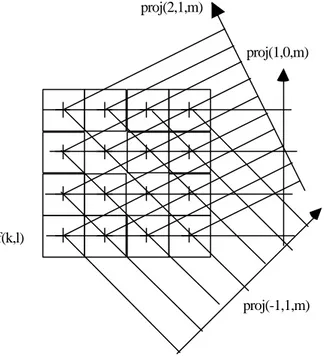
Figure 1 : 2D Mojette Transform from a 4×4 convex rectangular shape : a set of three projections has been computed.
proj(1,0,m)
f(k,l)
proj(-1,1,m) proj(2,1,m)
In the exemple of figure 1, 21 bins were computed for 16 pixels defining the shape. The redundancy of the
linear transform is then tuned according to the projection set choice and given by Red = #bins
#pixels - 1. The second
property is the angle-dependent projection sampling. As shown in Eqs. (3) and (4), the projection sampling
corresponds to the pixel center’s projection, as depicted in Figure 1.
To avoid ambiguities, only integer couples (p,q) with GCD(p,q) = 1 are taken as acceptable angles;
moreover, the q value is restricted to positive values. Another writing for Eq. (4) is
M f(k,l) = proj(p,q,b) = k
Σ
lΣ
f(k,l) ∆(b — P 21(
k l)
),with P21 = (–q p). (5)2.3 EQUIVALENT 3D MOJETTE DEFINITION
The Mojette transform definition in dimension 3 simply follows from Eq.(5). From a 3D convex volume
f(k,l,m), projections planes indexed by vector tB = (b1,b2) is given at angle (p,q,r) with GCD(p,q,r)=1 by :
proj(p,q,r,B) = M f(k,l,m) = k
Σ
lΣ
mΣ
f(k,l,m) ∆(B + P32(
k l m)),
(6)where P32 represents the projection matrix expression from the volume to the discrete plane indexed by vector B which is perpendicular to vector (p,q,r) and M is the mojette transform operator. The definition of
allowed angles followed the 2D case:
- r is always taken as positive,
- when r = 0, then q is taken as positive,
- last when q = r = 0 then p = 1.
The matrix expression is then defined by:
if r?0 and q?0 then P32
=
10 01 –p/r–q/r
, if r=0 and q?0 then P32=
10 –q/p0 01
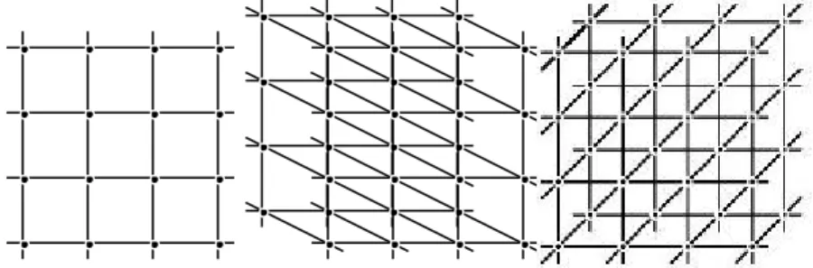
,It should be noticed that the angle-dependent sampling in 2D is translated as a specific grid in 3D as
exemplified by Figure 2. The generalization to nD Mojette transform is straightforward from the3D case.
Figure 2: 3D Mojette transform of a 4×4×4 mesh for angles (1 0 0), (–2 –1 1) and (1 1 2).
III Mojette reconstruction scheme
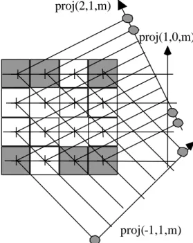
Figure 3 explains the mechanism of Mojette inversion. The gray corner pixels are in 1-1 correspondence
with their bins: these bin values can be backprojected and their value subtracted from all other projections. New
1-1 correspondences will appear. Iterating this process allows for the reconstruction of the whole convex region
(which has reduced to the empty set at the end of the process). In order to check if enough 1-1 correspondences
will appear for a given N×N square shape associated with a set of projections (pi,qi), the following formula due
to M. Katz [Katz 79] can be used:
N = Max ( P=
∑
i = 1 I |pi| ,Q=∑
i = 1. I |qi| ). (7)More general results for reconstructibility of any convex shapes have been found using mathematical
morphology [Normand Guédon 1998] by using two-pixel structuring elements dilations. The order of complexity
for a set of I projections obtained from a shape composed of N2 pixels is O(IN2) both for the direct and reverse
proj(1,0,m)
proj(-1,1,m)
proj(2,1,m)
Figure 3: the beginning of the inverse Mojette transform of figure 2.
IV FBP-Mojette
The filtered back-projection is the standard method applied in medical imaging devices such as CT
scanner, SPECT, or MRI. This section exhibits a new algorithm which can be considered as a mixture between
an angle-dependent version of the FBP for spline pixel intensity distribution model developed in [Guédon Bizais
1994] and the Mojette angular discrete version.
4.1 THE HAAR-MOJETTE TRANSFORM
The previous Mojette operator can not model a physical model of acquisition because of its discrete
version on the line of integration. In other words, the nuclear disintegration (SPECT, PET) or the X-rays
radiations are defined onto the real plane. Then, let restart with the Mojette transform when the interpolator of
Eq. (2) is defined as : ϕ0 (x) =
1 s i x< ½ ½ si x= ½ 0 sinon . (8)proj0 (b,p,q) = M0f(k,l)= Mδf(k,l) * kernel0(b,p,q) = proj−1 (b,p,q) * kernel0(b,p,q), (9) with kernel0(b,p,q)=
if p and q odd: (1 1 1 … 1) p * (1 1 1 …) q if p o r q even: ½ (1 1 1 … 1) p * (1 1 1 …) q * (1 1) (10)The interpolation kernel of Eq.(8) corresponds to a flat pixel. Thus the continuous line of integration of
the Radon transform is exactly transmitted to the sampled projection. Notice that only the previous Mojette
operator is needed and the additional convolution by the FIR filter defined in Eq. (10) can be simply done. The
inverse algorithm can also be used by recursively implementing the inverse filter (which only needs subtractions
because of the filter decomposition in Eq. 10) and then using the inverse Dirac-Mojette operator the initial image
can be recovered. In other words, the Mojette discrete version leads to a fast and exact algorithm compared to the
standard FBP algorithm.
4.2 THE FBP-MOJETTE ALGORITHM
The classical inverse Dirac-Mojette transform can not be used in case of non-exact reconstruction. As
soon as projections are not noise-free, the ill-posed nature of the inverse Radon transform appears. This has led
to use this instability for a watermarking scheme based on noisy Mojette projections [Autrusseau 2003].
The first operator that can be easily implemented is the exact discrete backprojector. It must be stressed
that even in [Guédon Bizais 1994] where the filter implementation for Haar-FBP was exact, its backprojection
counterpart was interpolated because of the sampling onto the projection which was pixel sampling dependent
but not angle-dependent. Remembering that the back-projection operator is the dual Radon operator defined in
the continuous case by :
g(x,y) = 1π
⌡
⌠
0π
proj(t, θ) dθ=R* proj(t, θ), (11)
its discrete Mojette version (the Mojette dual operator) is simply obtained by :
g(k,l) = 1 I
∑
i=1 I
proj(b,pi,qi) =M-1* proj(b,pi,qi). (12)
This version is adequate only because of the sampling onto the set of I projections S = {(pi,qi) i=1…I}.
derivation assumes an infinite number of angles leading to an angle independent definition. Here, we assume a
finite number of I directions and the corresponding sampling on these projections.
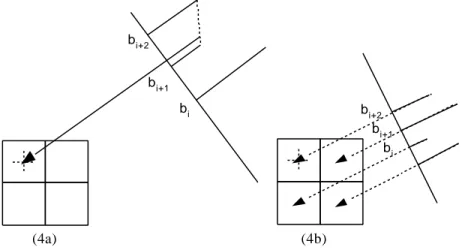
bi+1 bi bi+2 bi+1 bi bi+2 (4a) (4b)
Figure 4: 4.a : the interpolation onto the projection in order to backproject the right value at the corresponding center of the pixel. 4.b : the exact Mojette backprojector.
By reversing the order of the operators (to do a BPF instead of FBP) the 2D discrete filter h(k,l) that we
have to define corresponds to the response of the reconstruction scheme for a point spread function composed of
a single pixel (since we ensured linearity and shiftinvariantness). Thus h is given by the classical (discrete)
inverse filter equation:
g(k,l) ** h(k,l) = ∆(k) ∆ (l). (13)
In other words, the set S of discrete projections generate a specific discrete filter, which in turns, is related
to the geometry via the projection operator. Eq. (13) can not be inverted if the set S is not consistent with the size
of the convex shape we try to reconstruct (Katz’s formula). In the case where the Mojette inverse transform can
be performed, the Z transform will give the filter design. In the next section, the Mojette transform geometry is
used in conjunction with an ART-like (Algebraic Reconstruction Technique) algorithm.
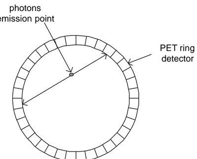
V Application to 3D PET geometry
For medical tomographic reconstruction, a specific area of work is the design of the 3D inverse Radon
transform corresponding to a Positron Emission Tomography (PET). In this case, a single point acquisition is
One desintegration leads to one hit for the two corresponding detectors. From these hits, projection planes
are computed. These projections with reconstruction algorithms (such as FBP algorithms) lead to backprojection
images.
PET ring
detector
photons
emission point
Figure 5: the geometry of a slice of 3D-PET acquisition .
The general geometry of PET acquisition has similarities with mojette geometry. Detector locations give
an initial discretization space. Then we have to find a mojette angle (p,q,r) spatially matching this couple of
detectors geometry. There are different (p,q,r) projection planes corresponding to the two detectors. The initial
location of the voxels will determine the incremented bin in the projection plane. Finally, for each desintegration
there is an incremented bin on a plane.
The way that Mojette geometry is used for 3D PET reconstruction is then to choose a set of possible
angles which has to be determined from a desired voxel resolution. Each detection leads to a (p,q,r) assignation
and a corresponding discrete bin position on the plane. The set of planes allowing a given resolution is fullfilled
with this algorithm. In another words, the approximation between original data and discrete data is minimized.
Nevertheless, there is missing data on PET projection plane and these datas are noisy. This prevent for a
standard inverse Mojette reconstruction. However, as seen in section 4, the Mojette backprojector corresponds to
an exact discrete operator. Since its Mojette projector counterpart is also exact, both discrete operators are used
The corresponding ART-like algorithm is iterative and each iteration is decomposed into a Mojette
backprojection step as in eq. (12), a projection step from the current reconstructed volume, and a difference
computation between previous and new projections data set.
VI Conclusion
In this paper, the discrete angle geometry was presented. Its direct application to define the Mojette
transform and its inverse was recalled. Its adequation to direct method was demonstrated using the FBP-Mojette
operators decomposition. This produces both a discrete exact backprojector associated with a discrete filter
defined from the set of available Mojette projections. Another important way of implementing the Mojette
transform in a noisy context was given with an ART-like algorithm in the context of 3D PET reconstruction. The
goal of the paper was to show that these exact discrete operators can be used both in direct and iterative
VII References
[Autrusseau Guédon 2003] : F. Autrusseau JP Guédon, “A cryptomarking algorithm for medical images using the Mojette transform,” SPIE Medical Imaging 2003, San Diego (CA), Vol., February 2003.
[Guédon Bizais 1994] : JP. Guédon, Y. Bizais, “ Bandlimited and Haar Filtered Back-Projection Reconstruction, ” IEEE Trans on Medical Imaging, Vol. 13 n° 3, pp. 430-440, September 1994.
[Guédon Normand 1997] : JP Guédon, N. Normand, “The Mojette transform ; applications for image analysis and coding,” VCIP 97, San Jose (CA), Vol. 3024, pp. 1220-1230, February 1997.
[Guédon and al 2001] : JP. Guédon, B. Parrein, N. Normand, "Internet distributed image information system” , Integrated Computer-Aided Engineering, vol. 8, p. 205-214, August 2001.
[Guédon Normand 2002] : JP Guédon, N. Normand, “Spline Mojette transform. Applications in tomography and communications,” Proc. EUSIPCO, September 2002.
[Katz 79] : M. Katz, Questions of Uniqueness and Resolution in Reconstruction from projections, Lecture Notes in Biomathematics, Springer-Verlag, Vol. 26, 1979.
[Normand Guédon 1998] : N. Normand, JP Guédon, “ The Mojette Transform : properties and implementation, ” Comptes-Rendus de l'Académie des Sciences de Paris, Computer science series, T. 336, pp.123–126, January 1998. [Philippé Guédon 1997] : O. Philippé, JP Guédon, “Correlation properties of the Mojette representation for non-exact image reconstruction,” Proc. Picture Coding Symposium 97, Berlin , ITG-Fachbericht Verlag Ed., pp.237-241, September 1997.
[Radon 1917]: J. Radon, “ Uber die Bestimmung von Functionen durch ihre Integralwerte langs gewisser Mannigfaltigkeiten, ” Berichte Sachsische Academie der Wissenchaften, Leipzig, Math. - Phys. Kl, vol 69 pp. 262-267, 1917.