HAL Id: hal-01056399
https://hal.archives-ouvertes.fr/hal-01056399
Submitted on 20 Aug 2014
HAL is a multi-disciplinary open access
archive for the deposit and dissemination of sci-entific research documents, whether they are pub-lished or not. The documents may come from
L’archive ouverte pluridisciplinaire HAL, est destinée au dépôt et à la diffusion de documents scientifiques de niveau recherche, publiés ou non, émanant des établissements d’enseignement et de
Accurate 3D Action Recognition using Learning on the
Grassmann Manifold
Rim Slama, Hazem Wannous, Mohamed Daoudi, Anuj Srivastava
To cite this version:
Rim Slama, Hazem Wannous, Mohamed Daoudi, Anuj Srivastava. Accurate 3D Action Recognition using Learning on the Grassmann Manifold. Pattern Recognition, Elsevier, 2015, 48 (2), pp.556-567. �hal-01056399�
Accurate 3D Action Recognition using Learning on the
Grassmann Manifold
Rim Slamaa,b, Hazem Wannousa,b, Mohamed Daoudib,c, Anuj Srivastavad
aUniversity Lille 1, Villeneuve d’Ascq, France
bLIFL Laboratory / UMR CNRS 8022, Villeneuve d’Ascq, France
cInstitut Mines-Telecom / Telecom Lille, Villeneuve d’Ascq, France dFlorida State University, Departement of Statistics, Tallahassee, USA
Abstract
In this paper we address the problem of modelling and analyzing hu-man motion by focusing on 3D body skeletons. Particularly, our intent is to represent skeletal motion in a geometric and efficient way, leading to an accurate action-recognition system. Here an action is represented by a dy-namical system whose observability matrix is characterized as an element of a Grassmann manifold. To formulate our learning algorithm, we pro-pose two distinct ideas: (1) In the first one we perform classification using a Truncated Wrapped Gaussian model, one for each class in its own tangent space. (2) In the second one we propose a novel learning algorithm that uses a vector representation formed by concatenating local coordinates in tangent spaces associated with di↵erent classes and training a linear SVM. We evaluate our approaches on three public 3D action datasets: MSR-action 3D, UT-kinect and UCF-kinect datasets; these datasets represent di↵erent
Email addresses: [email protected] (Rim Slama),
[email protected] (Hazem Wannous),
[email protected](Mohamed Daoudi), [email protected] (Anuj
kinds of challenges and together help provide an exhaustive evaluation. The results show that our approaches either match or exceed state-of-the-art per-formance reaching 91.21% on MSR-action 3D, 97.91% on UCF-kinect, and 88.5% on UT-kinect. Finally, we evaluate the latency, i.e. the ability to recognize an action before its termination, of our approach and demonstrate improvements relative to other published approaches.
Keywords: Human action recognition, Grassmann manifold, observational latency, depth images, skeleton, classification.
1. Introduction 1
Human action and activity recognition is one of the most active research 2
topics in the computer vision community due to its many challenging issues. 3
The motivation behind the great interest granted to action recognition is 4
the large number of possible applications in consumer interactive entertain-5
ment and gaming [1], surveillance systems [2], life-care and home systems 6
[3]. An extensive literature around this domain can be found in a number of 7
fields including pattern recognition, machine learning, and human-machine 8
interaction [4, 5]. 9
The main challenges in action recognition systems are the accuracy of 10
data acquisition and the dynamic modelling of the movements. The major 11
problems, which can alter the way actions are perceived and consequently 12
be recognized, are: occlusions, shadows and background extraction, lighting 13
condition variations and viewpoint changes. The recent release of consumer 14
depth cameras, like Microsoft Kinect, has significantly lighten these diffi-15
culties that reduce the action recognition performance in 2D video. These 16
cameras provide in addition to the RGB image a depth stream allowing to 17
discern changes in depth in certain viewpoints. 18
More recently, Shotton et al. [6] have proposed a real-time approach for 19
estimating 3D positions of body joints using extensive training on synthetic 20
and real depth-streams. The accurate estimation obtained by such a low-21
cost acquisition depth sensor has provided new opportunities for human-22
computer-interaction applications, where popular gaming consoles involve 23
the player directly in interaction with the computer. While these acquisition 24
sensors and their accurate data are within everyone’s reach, the next research 25
challenge is activity-driven. 26
In this paper we address the problem of modelling and analyzing human 27
motion in the 3D human joint space. Particularly, our intent is to represent 28
skeletal joint motion in a compact and efficient way that leads to an accurate 29
action recognition. Our ultimate goal is to develop an approach that avoids 30
an overly complex design of feature extraction and is able to recognize actions 31
performed by di↵erent actors in di↵erent contexts. 32
Additionally, we study the ability of our approach for reducing latency: 33
in other words, to quickly recognize human actions from the smallest number 34
of frames possible to permit a reliable recognition of the action occurring. 35
Furthermore, we analyze the impact of reducing the number of actions per 36
class in the training set on the classifier’s accuracy. 37
In our approach, the spatio-temporal aspect of the action is considered 38
and each movement is characterized by a structure incorporating the intrinsic 39
nature of the data. We believe that 3D human joint motion data captures 40
useful knowledge to understand the intrinsic motion structure, and a manifold 41
representation of such simple features can provide discriminating structure 42
for action recognition. This leads to manifold-based analysis, which has 43
been successfully used in many computer vision applications such as visual 44
tracking [7] and action recognition in 2D video [8, 9, 10, 11]. 45
Our overall approach is sketched in Figure 1, which has the following 46 modules: 47 Split Training videos Time series extrac on Temporal modelling Linear subspace representa on CT computa on LTB representa on S V M Evalua on LTB representa on Dataset Test videos Time series extrac on Temporal modelling Linear subspace representa on
Figure 1: Overview of the approach. The illustrated pipeline is composed of two main modules: (1) temporal modelling of time series data and manifold representation (2) learning approach on the Control Tangent spaces on Grassman manifold, using Local Bundle Tangent representation of data.
First, given training videos recorded from depth camera, motion trajecto-48
ries from the 3D human joint in Euclidean space are extracted as time series. 49
Then, each motion represented by its time series is expressed as an autore-50
gressive and moving average model (ARMA) in order to model its dynamic 51
process. The subspace spanned by columns of the observability matrix of 52
this model represents a point on a Grassmann manifold. 53
Second, using the Riemannian geometry of this manifold, we present a so-54
lution for solving the classification problem. We studied statistical modelling 55
of inter- and intra-class variations in conjunction with appropriate tangent 56
vectors on this manifold. While class samples are presented by a Grass-57
mann point cloud, we propose to learn Control Tangent (CT) spaces which 58
represent the mean of each class. 59
Third, each observation of the learning process is projected on all CTs 60
to form a Local Tangent Bandle (LTB) representation. This step allows 61
obtaining a discriminative parameterization incorporating class separation 62
properties and providing the input to a linear SVM classifier. 63
While given an unknown test video, to recognize its belonging to one of 64
N action classes, we apply the first step on the sequence to represent it as 65
a point on the Grassmann manifold. Then, this point is presented by its 66
LTB as done in learning step. In order to recognize the input action, SVM 67
classifier is performed. 68
The rest of the paper is organized as follows: In section 1, the state-of-69
the-art is summarized and main contributions of this paper are highlighted. 70
In section 2, parametric subspace-based modelling of 3D joint-trajectory is 71
discussed. In Section 3, statistical tools developed on a Grassmann manifold 72
are presented and a new supervised learning algorithm is introduced. In 73
Section 4, the strength of the framework in term of accuracy and latency on 74
several datasets are demonstrated. Finally, concluding remarks are presented 75
in Section 5. 76
2. Related works 77
In this section two categories of related works are reviewed from two 78
points of view: manifold-based approache and depth data representation. 79
We first review some related manifold based approaches for action analysis 80
and recognition in 2D video. Then we focus on the most recent methods of 81
action recognition from depth cameras. 82
2.1. Manifold approaches in 2D videos 83
Human action modelling from 2D video is a well studied problem in the 84
literature. Recent surveys can be found in the work of Aggarwal et al. [12], 85
Weinland et al. [13], and Poppe [4]. Beside classical methods performed 86
in Euclidean space, a variety of techniques based on manifold analysis are 87
proposed in recent years. 88
In the first category of manifold based approaches, each frame of action 89
sequence (pose) is represented as an element of a manifold and the whole 90
action is represented as a trajectory on this manifold. These approaches give 91
solutions in the temporal domain to be invariant to speed and time using 92
techniques like Dynamic Time Warping (DTW) to align action trajectories 93
on the manifold. Also probabilistic grammatical models like Hidden Markov 94
Model (HMM) are used to classify these actions presented as trajectories. 95
Indeed, Veeraraghavan et al. [14] propose the use of human silhouettes ex-96
tracted from video images as a representation of the pose. Silhouettes are 97
then characterized as points on the shape space manifold and modelled by 98
ARMA models in order to compare sequences using a DTW algorithm. In 99
another manifold shape space, Abdelkader et al. [15] represent each pose 100
silhouette as a point on the shape space of closed curves and each gesture is 101
represented as a trajectory on this space. To classify actions, two approaches 102
are used: a template-based approach (DTW) and a graphical model approach 103
(HMM). Other approaches use skeleton as a representation of each frame, as 104
works presented by Gong et al. [16]. They propose a spatio-Temporal Man-105
ifold (STM) model to analyze non-linear multivariate time series with latent 106
spatial structure and apply it to recognize actions in the joint-trajectories 107
space. Based on STM, they propose a Dynamic Manifold Warping (DMW) 108
and a motion similarity metric to compare human action sequences both in 109
2D space using a 2D tracker to extract joints from images and in 3D space 110
using Motion capture data. Recently, Gong et al. [17] propose a Kernelized 111
Temporal Cut (KTC) as an extension of their previous work [16]. They incor-112
porate Hilbert space embedding of distributions to handle the non-parametric 113
and high dimensionality issues. 114
Some manifold approaches represent the entire action sequence as a point 115
on an other special manifold. Indeed, Turaga et al. [18] involve a study of 116
the geometric properties of the Grassmann and Stiefel manifolds, and give 117
appropriate definitions of Riemannian metrics and geodesics for the purpose 118
of video indexing and action recognition. Then, in order to perform the clas-119
sification as a probability density function, a mean and a standard-deviation 120
are learnt for each class on class-specific tangent spaces. Turaga et al. [19] 121
use the same approach to represent complex actions by a collection of sub-122
sequence. These sub-sequences correspond to a trajectory on a Grassmann 123
manifold. Both DTW and HMM are used for action modelling and com-124
parison. Guo et al. [20] use covariance matrices of bags of low-dimensional 125
feature vectors to model the video sequence. These feature vectors are ex-126
tracted from segments of silhouette tunnels of moving objects and coarsely 127
capture their shapes. 128
Without any extraction of human descriptor as silhouette and neither an 129
explicit learning, Lui et al. [21] introduce the notion of tangent bundle to 130
represent each action sequence on the Grassmann manifold. Videos are ex-131
pressed as a third-order data tensor of raw pixel from action images, which 132
are then factorized on the Grassmann manifold. As each point on the mani-133
fold has an associated tangent space, tangent vectors are computed between 134
elements on the manifold and obtained distances are used for action clas-135
sification in a nearest neighbour fashion. In the same way, Lui et al. [22] 136
factorize raw pixel from images by high-order singular value decomposition 137
in order to represent the actions on Stiefel and Grassmann manifolds. How-138
ever, in this work where raw pixels are directly factorized as manifold points, 139
there is no dynamic modelling of the sequence. In addition, only distances 140
obtained between all tangent vectors are used for action classification and 141
there is no training process on data. 142
Kernels [23, 24] are also used in order to transform subspaces of a man-143
ifold onto a space where Euclidean metric can be applied. Shirazi et al. 144
[23] embed Grassmann manifolds upon a Hilbert space to minimize cluster-145
ing distortions and then apply a locally discriminant analysis using a graph. 146
Video action classification is then obtained by a Nearest-Neighbour classi-147
fier applied on Euclidean distances computed on the graph-embedded kernel. 148
Similarly, Harandi et al. [24] propose to represent the spatio-temporal as-149
pect of the action by subspaces elements of a Grassmann manifold. Then, 150
they embed this manifold into reproducing kernel of Hilbert spaces in order 151
to tackle the problem of action classification on such manifolds. Gall et al. 152
[25] use multi-view system coupling action recognition on 2D images with 153
3D pose estimation, were the action-specific manifolds are acting as a link 154
between them. 155
All these approaches cited above are based on features extracted from 156
2D video sequences as silhouettes or raw pixels from images. However, the 157
recent emergence of low-cost depth sensors opens the possibility of revisiting 158
the problem of activity modelling and learning using depth data-driven. 159
2.2. Depth data-driven approaches 160
Maps obtained by depth sensors are able to provide additional body shape 161
information to di↵erentiate actions that have similar 2D projections from a 162
single view. It has therefore motivated recent research works, to investigate 163
action recognition using the 3D information. Recent surveys [26, 27] are re-164
porting works on depth videos. First methods used for activity recognition 165
from depth sequences have tendency to extrapolate techniques already de-166
veloped for 2D video sequences. These approaches use points in depth map 167
sequences as a gray pixels in images to extract meaningful spatiotemporal 168
descriptors. In Wanqing et al. [28], depth maps are projected onto the three 169
orthogonal Cartesian planes (X Y , Z X, and Z Y planes) and the
170
contours of the projections are sampled for each frame. The sampled points 171
are used as bag-of-points to characterize a set of salient postures that corre-172
spond to the nodes of an action graph used to model explicitly the dynamics 173
of the actions. Local feature extraction approaches like spatiotemporal inter-174
est points (STIP) are also employed for action recognition on depth videos. 175
Bingbing et al.[29] use depth maps to extract STIP and encode Motion His-176
tory Image (MHI) in a framework combining color and depth information. 177
Xia et al [30] propose a method to extract STIP a on depth videos (DSTIP). 178
Then around these points of interest they build a depth cuboid similarity 179
feature as descriptor for each action. In the work proposed by Vieira et al. 180
[31], each depth map sequence is represented as a 4D grid by dividing the 181
space and time axes into multiple segments in order to extract SpatioTempo-182
ral Occupancy Pattern features (STOP). Also in Wang et al. [32], the action 183
sequence is considered as a 4D shape but Random Occupancy Pattern (ROP) 184
is used for features extraction. Yang et al.[33] employ Histograms of Oriented 185
Gradients features (HOG) computed from Depth Motion Maps (DMM), as 186
the representation of an action sequence. These histograms are then used as 187
input to SVM classifier. Similarly, Oreifej et al. [34] compute a 4D histogram 188
over depth, time, and spatial coordinates capturing the distribution of the 189
surface normal orientation. This histogram is created using 4D projectors 190
allowing quantification in 4D space. 191
The availability of 3D sensors has recently made possible to estimate 3D 192
positions of body joints. Especially thanks to the work of Shotton et al. 193
[6], where a real-time method is proposed to accurately predict 3D positions 194
of body joints. Thanks to this work, skeleton based methods have become 195
popular and many approaches in the literature propose to model the dynamic 196
of the action using these features. 197
Xia et al. [35] compute histograms of the locations of 12 3D joints as a 198
compact representation of postures and use them to construct posture visual 199
words of actions. The temporal evolutions of those visual words are modeled 200
by a discrete HMM. Yang et al. [36] extract three features, as pair-wise dif-201
ferences of joint positions, for each skeleton joint. Then, principal component 202
analysis (PCA) is used to reduce redundancy and noise from feature, and it 203
is also used to obtain a compact Eigen Joints representation for each frame. 204
Finally, a na¨ıve-Bayes nearest-neighbour classifier is used for multi-class ac-205
tion classification. The popular Dynamic Time Warping (DTW) technique 206
[37], well-known in speech recognition area, is also used for gesture and action 207
recognition using depth data. The classical DTW algorithm was defined to 208
match temporal distortions between two data trajectories, by finding an op-209
timal warping path between the two time series. The feature vector of time 210
series is directly constructed from human body joint orientation extracted 211
from depth camera or 3D Motion Capture sensors. Reyes et al. [38] per-212
form DTW on a feature vector defined by 15 joints on a 3D human skeleton 213
obtained using PrimeSense NiTE. Similarly, Sempena et al. [39], by the 3D 214
human skeleton model, use quaternions to form a 60-element feature vec-215
tor. The obtained warping path, by classical DTW algorithm, between two 216
time series is mainly subjected to some constraints: (1) boundary constraint 217
which enforces the first elements of the sequences as well as the last one 218
to be aligned to each other (2) monotonicity constraint which requires that 219
the points in the warping path are monotonically spaced in time in the two 220
sequences. This technique is relatively sensitive to noise as it requires all 221
elements of the sequences to be matched to a corresponding elements of the 222
other sequence. It also has a drawback related to its computational complex-223
ity incurring in quadratic cost. However, many works have been proposed to 224
bypass its drawbacks by means of probabilistic models [40] or incorporating 225
manifold learning approach [17, 16]. 226
Recent research has carried on more complex challenge of in-line recogni-227
tion systems for di↵erent applications, in which a trade-o↵ between accuracy 228
and latency can be highlighted. Ellis et al. [41] study this trade-o↵ and 229
employed a Latency Aware Learning (LAL) method, reducing latency when 230
recognizing actions. They train a logistic regression-based classifier, on 3D 231
joint position sequences captured by kinect camera, to search a single canon-232
ical posture for recognition. Another work is presented by Barnachon et 233
al. [42], where a histogram-based formulation is introduced for recognizing 234
streams of poses. In this representation, classical histogram is extended to 235
integral one to overcome the lack of temporal information in histograms. 236
They also prove the possibility of recognizing actions even before they are 237
completed using the integral histogram approach. Tests are made on both 3D 238
MoCap from TUM kitchen dataset [43] and RGB-D data from MSR-Action 239
dataset [28]. 240
Some hybrid approaches combining both skeleton data features and depth 241
information were recently introduced, trying to combine positive aspects of 242
both approaches. Azary et al. [44] propose spatiotemporal descriptors as 243
time-invariant action surfaces, combining image features extracted using ra-244
dial distance measures and 3D joint tracking. Wang et al. [45] compute 245
local features on patches around joints for human body representation. The 246
temporal structure of each joint in the sequence is represented through a tem-247
poral pattern representation called Fourier Temporal Pyramid. In Oreifej et 248
al. [34], a spatiotemporal histogram (HON4D) computed over depth, time, 249
and spatial coordinates is used to encode the distribution of the surface nor-250
mal orientation. Similarly to Wang et al. [45], HON4D histograms [34] are 251
computed around joints to provide the input of an SVM classifier. Althloothi 252
et al. [46] represent 3D shape features based on spherical harmonics repre-253
sentation and 3D motion features using kinematic structure from skeleton. 254
Both feature are then merged using multi kernel learning method. 255
It is important to note that, to date, few works have very recently pro-256
posed to use manifold analysis for 3D action recognition. Devanne et al. [47], 257
propose a spatiotemporal motion representation to characterize the action as 258
a trajectory which corresponds to a point on Riemannian manifold of open 259
curves shape space. These motion trajectories are extracted from 3D joints, 260
and the action recognition is performed by K-Nearest-Neighbor method ap-261
plied on geodesic distances obtained on open curve shape space. Azary et al. 262
[48] use a Grassmannian representation as an interpretation of depth motion 263
image (DMI) computed from depth pixel values. All DMI in the sequence 264
are combined to create a motion depth surface representing the action as a 265
spatiotemporal descriptor. 266
2.3. Contributions and proposed approach 267
On the one hand, approaches modelling actions as elements of manifolds 268
[49, 50, 9] prove that it is an appropriate way to represent and compare 269
videos. On the other hand, very few works deal with this task using depth 270
images and it is still possible to improve learning step using these models. 271
Besides, linear dynamic systems [51] show more and more promising results 272
on the motion modelling since they exhibit the stationary properties in time, 273
so they fit for action representation. 274
In this paper, we propose the use of geometric structure inherent in the 275
Grassmann manifold for action analysis. We perform action recognition by 276
introducing a manifold learning algorithm in conjunction with dynamic mod-277
elling process. In particular, after modelling motions as a linear dynamic sys-278
tems using ARMA models, we are interested in a representation of each point 279
on the manifold incorporating class separation properties. Our representa-280
tion takes benefit of statistics in the Grassmann manifold and action classes 281
representations on tangent spaces. From spatiotemporal point of view, each 282
action sequence is represented in our approach as linear dynamical system 283
acquiring the time series of 3D joint-trajectory. From geometrical point of 284
view, each action sequence is viewed as a point on the Grassmann manifold. 285
In terms of machine learning, a discriminative representation is provided for 286
each action thanks to a set of appropriate tangent vectors taking benefit 287
of manifold proprieties. Finally, the efficiency of the proposed approach is 288
demonstrated on three challenging action recognition datasets captured by 289
depth cameras. 290
3. Spatiotemporal modelling of action 291
The human body can be represented as an articulated system composed 292
of hierarchical joints that are connected with bones, forming a skeleton. The 293
two best-known skeletons provided by the Microsoft Kinect sensor, are those 294
obtained by official Microsoft SDK, which contains 20 joints, and PrimeSense 295
NiTE which contains only 15 joints (see Figure 2). The various joint con-296
figurations throughout the motion sequence produce a time series of skeletal 297
poses giving the skeleton movement. In our approach, an action is simply 298
described as a collection of time series of 3D positions of the joints in the 299
hierarchical configuration. 300
3.1. Linear dynamic model 301
Let pjt denote the 3D position of a joint j at a given frame t i.e., pj =
302
[xj, yj, zj]
j=1:J, with J is the number of joints. The joint position time-series
1 2 3 5 6 7 8 9 10 12 4 11 13 14 16 18 20 15 19 17 (a) 1 2 3 5 6 7 8 12 11 13 15 19 14 16 20 (b)
Figure 2: Skeleton joint locations captured by Microsof Kinect sensor (a) using Microsoft SDK (b) using PrimeSense NiTE. Joint signification are: (1) head (2) shoulder center (3) spine (4) hip center (5/6) left/right hip (7/8) left/ ight knee (9/10) left/right ankle (11/12) left/right foot (13/14) left/right shoulder (15/16) left/right elbow (17/19) left/right wrist (19/20) left/right hand.
of joint j is pjt = {xjt, yjt, ztj}t=1:Tj=1:J, with T the number of frames. A motion
304
sequence can then be seen as a matrix collecting all time-series from J joints, 305
i.e., M = [p1p2· · · pT], p 2 R3⇤J.
306
At this level, we could consider using DTW algorithm [37] to find optimal 307
non-linear warping function to match these given time-series as proposed by 308
[38, 39, 16]. However, we opted for a system combining a linear dynamic 309
modelling with statistical analysis on a manifold, avoiding the boundary and 310
the monotonicity constraints presented by classical DTW algorithm. Such a 311
system is also less sensitive to noise due to the poor estimation of the joint 312
locations, in addition to its reduced computational complexity. 313
The dynamic and the continuity of movement imply that the action can 314
not be resumed as a simply set of skeletal poses because of the temporal 315
information contained in the sequence. Instead of directly using original 316
joint position time-series data, we believe that a linear dynamic system, like 317
that often used for dynamic texture modelling, is essential before manifold 318
analysis. Therefore, to capture both the spatial and the temporal dynamics 319
of a motion, linear dynamical system characterized by ARMA models are 320
applied to the 3D joint position time-series matrix M . 321
The dynamic captured by the ARMA [52, 53] model during an action 322
sequence M can be represented as: 323
p(t) = Cz(t) + w(t), w(t)⇠ N(0, R),
z(t + 1) = Az(t) + v(t), v(t) ⇠ N(0, Q) (1)
where z 2 Rd is a hidden state vector, A2 Rd⇥d is the transition matrix
324
and C 2 R3⇤J⇥d is the measurement matrix. w and v are noise components
325
modeled as normal with mean equal to zero and covariance matrix R 2
326
R3⇤J⇥3⇤J and Q 2 Rd⇥d respectively. The goal is to learn parameters of the
327
model (A, C) given by these equations. Let UPVT be the singular value
328
decomposition of the matrix M . Then, the estimated model parameters A 329
and C are given by: ˆC = U and ˆA = PVTD
1V (VTD2V ) 1P 1, where
330
D1 = [0 0, I⌧ 1 0], D2 = [I⌧ 1 0, 0 0] and I⌧ 1 is the identity matrix of
331
size ⌧ 1.
332
Comparing two ARMA models can be done by simply comparing their 333
observability matrices. The expected observation sequence generated by an 334
ARMA model (A,C) lies in the column space of the extended observability 335
matrix given by ✓T
1 = [CT, (CA)T, (CA2)T, ...]T. This can be approximated
336
by the finite observability matrix ✓T
m = [CT, (CA)T, (CA2)T, ..., (CA2)m]T
[18]. The subspace spanned by columns of this finite observability matrix 338
corresponds to a point on a Grassmann manifold. 339
3.2. Grassmann manifold interpretation 340
Grassmannian analysis provides a natural way to deal with the problem of 341
sequence matching. Especially, this manifold allows to represent a sequence 342
by a point on its space and o↵ers tools to compare and to do statistics on 343
this manifold. The classification problem of sets of motions represented by a 344
collection of features can be transformed to point classification problem on 345
the Grassmann manifold. 346
In this work we are interested in Grassmann manifolds which definition 347
is as below. 348
Definition: The Grassmann manifold Gn⇥d is a quotient space of orthogonal
349
group O(n) and is defined as the set of d-dimensional linear subspaces of Rn.
350
Points on the Grassmann manifold are equivalent classes of n⇥ d orthogonal
351
matrices, with d < n, where two matrices are equivalent if their columns span 352
the same d-dimensional subspace. 353
Let µ denotes an element on Gn⇥d, the tangent space to this element Tµ on
354
Gn,d is the tangent plane to the surface of the manifold at µ. It is possible
355
to map a point U , of the Grassmann manifold, to a vector in the tangent 356
space Tµ using the logarithm map as defined by Turaga et al. [18]. An other
357
important tool in statistics is the exponential map Expµ : Tµ(Gn,d) ! Gn,d,
358
which allows to move on the manifold. 359
Two points U1 and U2 on Gn,d are equivalent if one can be mapped into
360
the other one by d⇥ d orthogonal matrix [54]. In other words, U1 and U2 are
361
equivalent if the d columns of U1 are rotations of U2. The minimum length
curve connecting these two points is the geodesic between them computed 363
as: 364
dgeod(U1, U2) =k [✓1, ✓2,· · · , ✓i,· · · , ✓d]k2 (2)
where ✓i is the principal angle vector which can be computed through the
365
SVD of UT
1 U2.
366
4. Learning process on the manifold 367
Let {U1,· · · UN} be N actions represented by points on the Grassmann
368
manifold. A common learning approach on manifolds is based on the use 369
of only one-tangent space, which usually can be obtained as the tangent 370
space to the mean (µ) of the entire data points {Ui}i=1:N without regard
371
to class labels. All data points on the manifold are then projected on this 372
tangent space to provide the input of a classifier. This assumption provide an 373
accommodated solution to use a classical supervised learning on the manifold. 374
However, this flattening of the manifold through tangent space is not efficient 375
since the tangent space on the global mean can be far from other points. 376
A more appropriate way is to consider separate tangent spaces for each 377
class at the class-mean. The classification is then performed in these indi-378
vidual tangent spaces as in [18]. 379
Some other approaches explore the idea of tangent bundle as in Lui et 380
al. [21, 22], in which all tangent planes of all data points on the manifold 381
are considered. Tangent vectors are then computed between all points on 382
a Grassmann manifold and action classification is performed thanks to ob-383
tained distances. 384
We believe that using several tangent spaces, obtained for each class of 385
the training data points, is more intuitive. However, the question here is how 386
to learn a classifier in this case? 387
In the rest of the section, we present a statistical computation of the mean 388
in the Grassmann manifold [55]. Then, we propose two learning methods on 389
this manifold taking benefit from tangent space class specific and tangent 390
bundle [21]: Truncated Wrapped Gaussian (TWG) [56] and Local Tangent 391
Bundle SVM (LBTSVM). 392
4.1. Mean computation on the Grassmann manifold 393
The Karcher mean [55] enables computation of a mean representative for 394
a cluster of points on the manifold. This mean should belong to the same 395
space as the given points. In our case, we need Karcher mean to compute 396
averages on the Grassman manifold and more precisely means of each action 397
class which represents the action at best. The algorithm exploits log and exp 398
maps in a predictor/corrector loop until convergence to an expected point. 399
The computation of a mean can be used to perform an action classification 400
solution. This can be done by a s simple comparison of an unknown action, 401
represented as a point on the manifold, to all class-means and assigning it to 402
the nearest one using the distance presented in Equation 2. 403
4.2. Truncated Wrapped Gaussian 404
In addition to the mean µ computed by Karcher mean on {Ui}i=1:N, we
405
look for the standard deviation value between all actions in each class of
406
training data. The must be computed on {Vi}i=1:N where V = expµ1(Ui)
407
are the projections of actions from the Grassmann manifold into the tangent 408
space defined on the mean µ. The key idea here is to use the fact that the 409
tangent space Tµ(Gn,d) is a vector space.
410
Thus, we can estimate the parameters of a probability density function 411
such as a Gaussian and then use the exponential map to wrap these param-412
eters back onto the manifold using exponential map operator [18]. However, 413
the exponential map is not a bijection for the Grassmann manifold. In fact, a 414
line on tangent space, with infinite length, can be warpped around the man-415
ifold many times. Thus, some points of this line are going to have more than 416
one image on Gn,d. It becomes a bijection only if the domain is restricted.
417
Therefore, we can restrict the tangent space by a truncation beyond a radius 418
of ⇡ in Tµ(Gn,d). By truncation, the normalization constant changes for
mul-419
tivariate density in Tµ(Gn,d). In fact, it gets scaled down depending on how
420
much of the probability mass is left out of the truncation region. 421
Let f (x) denotes the probability density function (pdf) defined on Tµ(Gn,d)
422 by : 423 f (x) = p 1 2⇡ 2e x2 2 2 (3)
After truncation, an approximation of f gives: 424
ˆ
f (x) = f (x)⇥
1
|x|<⇡z (4)
where z is the normalization factor : 425
z =
Z ⇡
⇡
f (x)⇥
1
|x|<⇡dx (5)Using Monte Carlo estimation, it can proved that the estimation of z is given 426
by: 427 ˆ z = 1 N N X i=1
1
|xi|<⇡ (6)In practice, we employ wrapped Gaussians in each class-specific tangent 428
space. Separate tangent space is considered for each class at its mean com-429
puted by Karcher mean algorithm. Predicted class of an observation point 430
is estimated in these individual tangent spaces. In the training step, the 431
mean, standard deviation and normalization factor in each class of actions 432
are computed. The predicted label of unknown class action is estimated as 433
a function of probability density in class-specific tangent spaces. 434
4.3. Local Tangent Bundle 435
We intent here to generalize a learning algorithm to work with data points 436
which are geometrically lying to a Grassmann manifold. Using multiple class-437
specific tangent spaces is decidedly more relevant than single one. However, 438
restrict the learning to only the mean and the standard-deviation in each tan-439
gent space, as in TGW method, is probably insufficient to classify complex 440
actions with small inter-class variation. Our idea is to build a supervised clas-441
sifier on the manifold but without limiting the learning process to distances 442
computed on the tangent spaces as in [22]. 443
We consider such data points to be embedded in higher dimensional rep-444
resentation providing a natural and implicit separation of directions. We 445
use the notion of tangent bundle on the manifold to formulate our learning 446
algorithm. 447
The tangent bundle of a manifold is defined in the literature as the mani-448
fold along with the set of tangent planes taken at all points on it. Each such 449
a tangent plane can be equipped with a local Euclidean coordinate system. 450
In our approach, we consider several ”local” bundles, each one represents the 451
tangent planes taken at all points belonging to a class from training dataset 452
and expressed as class-specific local bundle. 453
We generate Control Tangents (CT) on the manifold, which represent 454
all class-specific local bundles of data points. Each CT can be seen as the 455
tangent space of the Karcher mean of all points belonging to the same class 456
of points from only training data. Karcher mean algorithm can be employed 457
here for mean computation. 458
We introduce an upswing of the manifold learning so-called Local Tangent 459
Bundle (LTB), in which proximities are required between each point on the 460
manifold and all CTs. The LTB can be viewed as a parameterization of 461
a point on the manifold which incorporates implicitly release properties in 462
relation to all class clusters, by mapping this point to all CTs using logarithm 463
map. 464
The LTBs can provide the input of a classifier, like the linear SVM clas-465
sifier as in our case. In doing so, the learning model of the classifier is con-466
structed using LTBs instead of classifying as function of the local distances 467
(mean and standard-deviation) of the point from LTBs as in TWG method. 468
We finally notice that training a linear SVM classifier on our represen-469
tation of points provided by LTB is more appropriate than the use of SVM 470
with classical Kernel, like rbf, on original points on the manifold. 471
In experiments, we compare our learning approach LTBSVM to the clas-472
sical one denoted as One-tangent SVM (TSVM), in which the mean is com-473
puted on the entire training dataset regardless to class labels. Then, all 474
points on the manifold are projected on this later to provide the inputs of a 475
linear SVM. 476
A graphical illustration of the manifold learning by TWG and LTB can 477
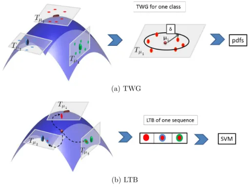
be shown in Figure 3. 478
(a) TWG
(b) LTB
Figure 3: Conceptual TWG and LTB learning methods on the Grassmann manifold.
(a) Actions belonging to the same class, illustrated with same color, are projected to the tangent space presented with their mean and then Gaussian function is computed on each tangent space, (b) An action is projected on all CTs, and thus construct a new observation is represented by its LTB.
5. Experimental results 479
This section summarizes our empirical results and provides an analysis of 480
the performances of our proposed approach on several datasets compared to 481
the state-of-the-art approaches. 482
5.1. Data and features 483
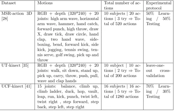
We extensively experimented our proposed approach on three public 3D 484
action datasets containing various challenges, including MSR-action 3D [28], 485
UT-kinect [35] and UCF-kinect [41]. All details about these datasets: di↵er-486
ent types and number of motions, number of subjects executing these motions 487
and the experimental protocol used for evaluation are summarized in Table 488
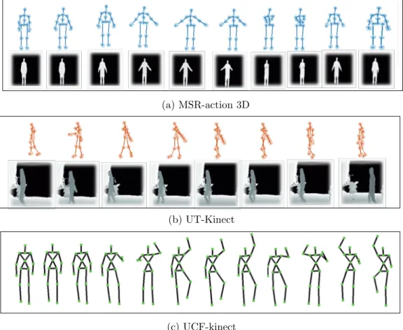
1. Examples of actions from these datasets are shown in Figure 4. 489
Dataset Motions Total number of
ac-tions Experimental protocol MSR-action 3D [28] RGB + depth (320*240) + 20 joints: high arm wave, horizontal arm wave, hammer, hand catch, forward punch, high throw, draw X, draw tick, draw circle, hand
clap, two hand wave,
side-boxing, bend, forward kick, side kick, jogging, tennis swing, ten-nis serve, golf swing, pick up and throw
10 subjects| 20 ac-tions| 3 try ) To-tal of 520 actions
50%
Learn-ing / 50%
Testing
UT-kinect [35] RGB + depth (320*240) + 20
joints: walk, sit down, stand up, pick up, carry, throw, push, pull, wave and clap hands
10 subject | 10 ac-tions| 2 try ) To-tal of 200 actions
leave-one-out
cross-validation
UCF-kinect [41] 15 joints: balance, climb up,
climb ladder, duck, hop, vault, leap, run, kick, punch, twist left, twist right , step forward, step back, step left, step right
16 subjects| 16 ac-tions| 5 try ) To-tal of 1280 actions
70%
Learn-ing / 30%
Testing
Table 1: Overview of the datasets used in the experiments.
In all these datasets, a normalization step is performed in order to make 490
the skeletons scale-invariant. For each frame, the hip center joint is first 491
placed at the origin of the coordinate system. Then, a skeleton template is 492
taken as reference and all the other skeletons are normalized such that their 493
(a) MSR-action 3D
(b) UT-Kinect
(c) UCF-kinect
Figure 4: Examples of human actions from datsets used in our experiments: (a) ’hand clap’ from MSR-action 3D , (b) ’walk’ from UT kinect and (c) ’climb ladder’ from UCF-kinect.
body part lengths are equal to the corresponding lengths of the reference 494
skeleton. Each 3D joint sequence is represented as time series matrix of size 495
F ⇥ T with T the number of frames in the sequence and F the number
496
of features per frame. The number of features depends on the number of 497
estimated joints (60 values for Microsoft SDK skeleton and 45 for PrimeSense 498
NiTE skeleton). The dynamic of the activity is then captured using an 499
ARMA model. In this process, a dimensionality reduction is needed and best 500
subspace dimension ”d” have been chosen using a 5-fold cross-validation on 501
the training dataset. The parameter giving the best accuracy on the training 502
set is kept for all experiments. 503
Each action is an element of the Grassmann manifold Gn⇥dwith n = m⇥J
504
where J represents the number of joints and d is the subspace dimension 505
learnt on the training data. We set m = d, while m represents the truncation 506
parameter of observation. 507
In our LTBSVM approach, we train a linear SVM on our LTB represen-508
tations of points on the Grassmann manifold. We use a multi-class SVM 509
classifier from LibSVM library [57], where the penalty parameter C is tuned 510
using a 5-fold cross-validation on the training dataset. 511
We evaluate the performance of our approach for action recognition and 512
explore the latency on recognition by evaluating the trade-o↵ between accu-513
racy and latency over varying number of actions. To allow a better evalua-514
tion of our approach, we conducted experiments respecting those made in the 515
state-of-the-art approaches. We note here that other interesting datasets are 516
available, like TUM kitchen dataset [43] which presents challenging short and 517
complex actions. In our experiments we concentrated on three other datasets 518
from depth sensors (such as kinect), chosen according to the challenges they 519
contain, as occlusion, change of view and possibility to compare the latency. 520
Details of the experiments are presented in the following sections. 521
5.2. MSR-Action 3D dataset 522
MSR-Action 3D [28] is a public dataset of 3D action captured by a depth 523
camera. It consists of a set of temporally segmented actions where subjects 524
are facing the camera and they are advised to use their right arm or leg if 525
an action is performed by a single limb. The background is pre-processed 526
clearing discontinuities and there is no interaction with objects in performed 527
actions. Despite of all of these facilities, it is also a challenging dataset 528
since many activities appear very similar due to small inter-class variation. 529
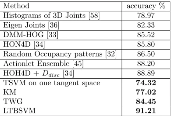
Several works have already been conducted on this dataset. Table 2 shows 530
the accuracy of our approach compared to the state-of-the-art methods. We 531
followed the same experimental setup as in Oreifej et al. [34] and Jiang et 532
al. [45], where first five actors are used for training and the rest for testing. 533
Our results obtained in this table correspond to four learning methods: 534
simple Karcher Mean (KM), one Tangent SVM (TSVM), Truncated Wrapped 535
Gaussian (TWG) and Local Tangent Bundle SVM (LTBSVM). Our approach 536
using LTBSVM achieves an accuracy of 91.21%, exceeding the best method 537
from the state-of-the-art proposed by Oreifej et al. [34]. We note that our 538
approach is based on only skeletal joint coordinates as motion features, com-539
pared to other approaches, such as Oreifej et al. [34] and Wang et al. [32] 540
which use the depth map or depth information around joint locations. 541
To evaluate the e↵ect of the changing of the subspace dimensions, we 542
conduct several tests on MSR-Action 3D dataset with di↵erent dimensions 543
Method accuracy %
Histograms of 3D Joints [58] 78.97
Eigen Joints [36] 82.33
DMM-HOG [33] 85.52
HON4D [34] 85.80
Random Occupancy patterns [32] 86.50
Actionlet Ensemble [45] 88.20
HOH4D + Ddisc [34] 88.89
TSVM on one tangent space 74.32
KM 77.02
TWG 84.45
LTBSVM 91.21
Table 2: Recognition accuracy (in %) for the MSR-Action 3D dataset using our approach compared to the previous approaches.
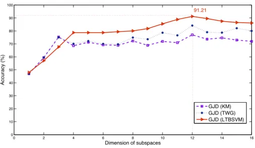
of subspaces. Figure 5 shows the variation of recognition performances with 544
the change of the subspace dimension. We remark that until dimension 12, 545
the recognition rate generally increase with the increase of the size of the 546
subspaces dimensions. This is expected, since a small dimension causes a 547
lack of information but also a big dimension of the subspace keeps noise and 548
brings confusion between inter-classes. We also compare in this figure, our 549
new introduced learning algorithm LBTSVM to TWG and KM. 550
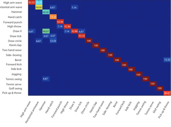
To better understand the behavior of our approach according to the action 551
type, the confusion matrix is illustrated in Figure 6. For most actions, about 552
11 classes of actions, video sequences are 100% correctly classified. 553
The classification error occurs if two actions are very similar, such as 554
’horizontal arm wave’ and ’high arm wave’. Besides, one of most problematic 555
action to classify is ’hammer’ action which is frequently confused with ’draw 556
X’. The particularity of these two actions is that they start in the same 557
way but one finishes before the other. If we show only the first part of 558
’draw X’ action and the whole sequence of ’hammer’ action we can see that 559
0 2 4 6 8 10 12 14 16 0 10 20 30 40 50 60 70 80 90 100 Dimension of subspaces Accuracy (%) GJD (KM) GJD (TWG) GJD (LTBSVM) 91.21
Figure 5: Recognition rate variation with learning approach and subspace dimension.
they are very similar. The same for ’hand catch’ action which is confused 560
with ’draw circle’. It is important to note that ’hammer’ action is completely 561
misclassified with the approach presented by Oreifej et al. [34] which presents 562
the second better recognition rate after our approach. 563
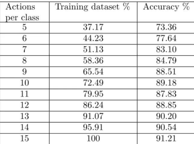
While the focus of this paper is mainly on action recognition and latency 564
reduction, some applications need to perform training step with a reduced 565
amount of data. To study the e↵ect of the amount of training dataset, we 566
measured how the accuracy changed as we iteratively reduced the number of 567
actions per class in the training dataset. Table 3 shows obtained accuracy 568
results with di↵erent size of training dataset. 569
These results show that, in contrast to approaches that use HMM which 570
require a large number of training data, our approach reveals robustness and 571
efficiency. This robustness is due to the fact that the Control Tangents, which 572
93.33 33.33 60.00 40.006.67 7.14 73.33 92.86 7.14 92.86 6.67 46.67 6.67 7.14 92.866.67 6.67 93.33 6.67 13.33 100 100 100 100 100 100 13.33 100 100 6.67 100 100 100 86.67
High arm wave
High arm wave
Horizontal arm wave
Horizontal armwave Hammer Hammer Hand catch Hand catch Forward punch Forward punch High throw High throw Draw X Draw X Draw tick Draw tick Draw circle Draw circle Hand clap Hand clap
Two hand wave
Tow hand wave
Side−boxing Side −boxing Bend Bend Forward kick Forward kick Side kick Side kick Jogging Jogging Tennis swing Tennis swing Tennis serve Tennis serve Golf swing Glof swing
Pick up & throw
Pick up & throw
Figure 6: The confusion matrix for the proposed approach on MSR-Action 3D dataset.
It is recommended to view the Figure on the screen.
play an important role in learning process, can be computed efficiently using 573
small number of action points per class on the manifold. 574
5.3. UT-Kinect dataset 575
Sequences of this dataset are taken using one depth camera (kinect) in 576
indoor settings and their length vary from 5 to 120 frames. We use this 577
dataset because it contains several challenges: 578
• View change, where actions are taken from di↵erent views: right view, 579
frontal view or back view. 580
Actions per class
Training dataset % Accuracy %
5 37.17 73.36 6 44.23 77.64 7 51.13 83.10 8 58.36 84.79 9 65.54 88.51 10 72.49 89.18 11 79.95 87.83 12 86.24 88.85 13 91.07 90.20 14 95.91 90.54 15 100 91.21
Table 3: Recognition accuracy, obtained by our approach using LTBSVM on MSR-Action 3D dataset, with di↵erent size of training dataset.
• Significant variation in the realization of the same action: same action 581
is done with one hand or two hands can be used to describe the ’pick 582
up’ action. 583
• Variation in duration of actions: the mean and standard-deviation are 584
respectively for the whole actions 31.1 and 11.61 frames at 30 fps. 585
To compare our results with state-of-the-art approaches, we follow experi-586
ment protocol proposed by Xia et al. [35]. The protocol is leave-one-out 587
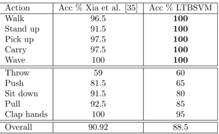
cross-validation. In Table 4, we show comparison between the recognition 588
accuracy produced by our approach and the approach presented by Xia et 589
al. [35]. 590
This table shows the accuracy of the five least-recognized actions in UT-591
kinect dataset and the five best-recognized actions. Our system performs 592
the worst when the action represents an interaction with an object: ’throw’, 593
’push’, ’sit down’ and ’pick up’. However, for the best five recognized actions, 594
our approach improves the recognition rate reaching 100%. These actions 595
Action Acc % Xia et al. [35] Acc % LTBSVM Walk 96.5 100 Stand up 91.5 100 Pick up 97.5 100 Carry 97.5 100 Wave 100 100 Throw 59 60 Push 81.5 65 Sit down 91.5 80 Pull 92.5 85 Clap hands 100 95 Overall 90.92 88.5
Table 4: Recognition accuracy (per action) for the UT-kinect dataset obtained by our approach using LTBSVM compared to Xia et al. [35].
contain variations in view point and realization of the same action. This 596
means that our approach is view-invariant and it is robust to change in action 597
types thanks to the used learning approach. The overall accuracy of Xia et al. 598
[35] is better than our recognition rate. However on MSR Action3D database, 599
the recognition rate obtained by this approach gives only 78.97%. This can 600
be explained by the fact that this approach requires a large training dataset. 601
Especially for complex actions which a↵ect adversely the HMM classification 602
in case of small samples of training. 603
5.4. UCF-kinect dataset 604
In this experiment, our approach is evaluated in terms of latency, i.e. 605
the ability for a rapid (low-latency) action recognition. The goal here is to 606
automatically determine when a sufficient number of frames are observed to 607
permit a reliable recognition of the occurring action. For many applications, 608
a real challenge is to define a good compromise between ”making forced de-609
cision” on partial available frames (but potentially unreliable) and ”waiting” 610
for the entire video sequence. 611
To evaluate the performance of our approach in reducing latency, we con-612
ducted our experiments on UCF-kinect dataset [41]. The skeletal joint loca-613
tions (15 joints) over sequences of this dataset are estimated using Microsoft 614
Kinect sensor and the PrimeSense NiTE. The same experimental setup as 615
in Ellis et al. [41] is followed. For a total of 1280 action samples contained 616
in this dataset, a 70% and 30% split is used for respectively training and 617
testing datasets. From the original dataset, new subsequences were created 618
by varying a parameter corresponding to the K first frames. Each new sub-619
sequence was created by selecting only the first K frames from the video. For 620
videos shorter than K frames, the entire video is used. We compare the re-621
sult obtained by our approach to those obtained by Latency Aware Learning 622
(LAL) method proposed by Ellis et al. [41] and other baseline algorithms: 623
Bag-of-Words (BoW) and Linear Chain Conditional Random Field (CRF), 624
also reported by Ellis et al. [41]. 625
As shown in Figure 7, our approach using LTBSVM clearly achieves im-626
proved latency performance compared to all other baseline approaches. Anal-627
ysis of these curves shows that, accuracy rates for all other approaches are 628
close when using small number of frames (less than 10) or a large number of 629
frames (more than 40). However, the di↵erence increases significantly in the 630
middle range. The table joint to Figure 7 shows numerical results at several 631
points along the curves in the figure. Thus, given only 20 frames of input, 632
our system achieves 74.37%, while BOW, CRF recognition rate below 50% 633
and LAL achieves 61.45%. 634
It is also interesting to notice the improvement of accuracy of 92.08% 635
0 10 20 30 40 50 60 0 10 20 30 40 50 60 70 80 90 100 Maximum frames Accuracy (% ) LTBSVM LAL TWG CRF BoW Approach/frames 10 15 20 25 30 40 60 LTBSVM 21.87 49.37 74.37 86.87 92.08 97.29 97.91 TWG 18.95 40.62 61.45 74.79 82.7 92.29 95.62 LAL [41] 13.91 36.95 64.77 81.56 90.55 95.16 95.94 CRF [41] 14.53 25.46 46.88 67.27 80.70 91.41 94.06 BOW [41] 10.7 21.17 43.52 67.58 83.20 91.88 94.06
Figure 7: Accuracy vs. state-of-the-art approaches over videos truncated at varying maxi-mum lengths. Each point of this curve shows the accuracy achieved by the classifier given only the number of frames shown in the x-axis.
obtained by LTBSVM compared to 82.7% obtained by TWG, with maximum 636
frame number equal to 30. For a large number of frames, all of the methods 637
perform globally a good accuracy with an improvement of the ours (97.91% 638
comparing to 95.94% obtained by LAL proposed in Ellis et al. [41]). These 639
results show that our approach can recognize actions at the desired accuracy 640
with reducing latency. 641
Finally, the detail of recognition rates, when using the totality of frames 642
in the sequence, are shown through the confusion matrix in Figure 8. Unlike 643
what gives LAL, we can observe that the ’twist left’, ’twist right’ actions are 644
not confused with each others. All classes of actions are classified with a rate 645
more than 93.33% which gives a lot of confidence to our proposed learning 646 approach. 647 100 100 93.33 3.33 100 3.33 93.33 100 6.67 3.33 96.67 100 3.33 100 93.33 3.33 100 100 3.33 100 100 3.33 93.33 3.33 96.67 balance balance climbladder climbladder climbup climbup duck duck hop hop kick kick leap leap punch punch run run stepback stepback stepfront stepfront stepleft stepleft stepright stepright twistleft twistleft twistright twistright vault vault
Figure 8: The confusion matrix for the proposed method on UCF-kinect dataset. Overall
accuracy achieved 97.91%. It is recommended to view the figure on the screen.
5.5. Discussion 648
Manifold representation and learning. Data representation is one of the most 649
important factors in the recognition approach, on which we must take a lot 650
of consideration. Our data representation, like many state-of-the-art man-651
ifold techniques [19, 14, 21], consider the geometric space and incorporates 652
the intrinsic nature of the data. In our framework, which is 3D joint-based, 653
both geometric appearance and dynamic of human body are captured simul-654
taneously. Furthermore, unlike the manifold approaches using silhouettes 655
[14, 15, 18], or directly raw pixels [22, 19], our approach use informative 656
geometric features, which capture useful knowledge to understand the in-657
trinsic motion structure. Thanks to recent release of depth sensor, these 658
features are extracted and tracked along the action sequence, while classical 659
pixel-based manifold approaches relying on a good action localization, or on 660
tedious feature extraction from 2D videos like silhouettes. 661
In terms of learning method, we generalized a learning algorithm to work 662
with data points which are geometrically lying to a Grassmann manifold. 663
Other approaches are tested in the learning process on the manifold: one 664
tangent space (TSVM) and class-specific tangent spaces (TWG). In the first 665
one, recognition rate is low. In fact, the computation of the mean of all 666
actions from all classes can be inaccurate. Besides, projections on this plane 667
can lead to big deformations. A better solution is to operate on each class by 668
computing its proper tangent space, as in TWG [56] which improve TSVM 669
results (see Table 2). In our approach (LTBSVM), both Control Tangent 670
and statistics on the manifold are used. The purpose was to formulate our 671
learning algorithm using a discriminative parametrization which incorporate 672
class separation properties. The particularity of our learning model is the 673
incorporation of proximities relative to all Control Tangent spaces represent-674
ing class clusters, instead of classifying using a function of local distances. 675
The results in Table 2 demonstrate that the proposed algorithm is more effi-676
cient in action recognition scenario when inter-variation classes is present as 677
a challenge. 678
Furthermore, the analysis of the impact of reducing the number of actions 679
in the training set on the accuracy of the classifier show robustness. Even 680
with a small number of actions in the training data recognition rates remain 681
good as demonstrated in Table 3. However it is a limitation especially for 682
approaches using an HMM learning because they require a large number of 683
training dataset. Such as Xia et al. approach [35], which gives only 78.97% 684
of recognition rate while performing cross subject test on MSR dataset. 685
Latency and Time computation. The evaluations in terms of latency have 686
clearly revealed the efficiency of our approach for a rapid recognition. It 687
is possible to recognize actions up to 95% using only 40 frames which is 688
a good performance comparing to state-of-the-art approaches presented in 689
[41]. Thus, our approach can be used for interactive systems. Particularly, 690
in entertainment applications to resolve the problem of lag and improve some 691
motion-based games. 692
Since the proposed approach is based on only skeletal joint coordinates, 693
it is simple to calculate and it needs only a small computation time. In fact, 694
with our current implementation written in C++, the whole recognition time 695
takes 0.26 sec to recognize a sequence of 60 frames. The joint extraction and 696
normalisation take 0.0001 sec, the Grassmann and the LTB representation 697
take 0.0108 sec and the prediction on SVM takes 0.251 sec. These computa-698
tion time are reported on UCF dataset, with Grassmann manifold dimension 699
n = 540 and d = 12. We also reported the computation time needed to 700
recognize actions while incorporating latency on UCF dataset. Figure 9 il-701
lustrates inline time recognition with time progression, after only 40 frames 702
the recognition is given at the 0.94 sec within 97.29% of correctness rate. 703
After 60 frames, in 1.3 sec the algorithm recognize correctly the action with 704
97.91%. All the computation time experiments are lunched on a PC having 705
Intel Core i5-3350P (3.1 GHz) CPU, 4GB RAM and a PrimeSense camera 706
for skeleton extraction giving about 60 skeleton/sec. 707
0
20
40
60
Frame number…
…
…
0
0.66
0.94
1.31
Inline me recogni on(secondes) Recogni on me: 0.26 sec
Figure 9: The computation time to perform 20 frames actions sequences is 0.26 sec by
using our approach. The computation time is given for each actions frames sequences (e.g. 0.94 sec for 40 frames).
Limitations. Our proposed approach is a 3D joint-based framework derives 708
a human action recognition from skeletal joint sequences. In the case of 709
presence of object interaction in human actions, our approach do not provides 710
any relevant information about objects and thus, action with and without 711
objects are confused. This limitation can be leveraged in future by the use 712
of additional features, which can be extracted from depth or color images 713
associated to 3D joint locations. 714
6. Conclusion 715
In this paper, an e↵ective framework for modelling and recognizing hu-716
man motion in the 3D skeletal joint space is proposed. In this framework, 717
sequence features are modeled temporally as subspaces lying to a Grassman-718
nian manifold. A new learning algorithm on this manifold is then introduced. 719
It embeds each action, presented as a point on the manifold, in higher dimen-720
sional representation providing natural separation directions. We formulated 721
our learning algorithm using the notion of local tangent bundles on class clus-722
ters on the Grassmann manifold. The empirical results and the analysis of 723
the performance of our proposed approach show promising results with high 724
accuracies superior to 88% on three di↵erent datasets. The evaluation of 725
our approach in terms of accuracy/latency reveals an important ability for 726
a low-latency action recognition system. Obtained results show that with 727
minimum number of frames, it provides the highest recognition rate. 728
We would encourage future works to extend our approach to investigate 729
more challenging problems like human behaviour recognition. Finally, we 730
plan to use additional features from depth or color images associated to 3D 731
joint locations to solve the problem of human-object interaction. 732
References 733
[1] S. Fothergill, H. Mentis, P. Kohli, S. Nowozin, Instructing people for 734
training gestural interactive systems, in: CHI Conference on Human 735
Factors in Computing Systems, New York, NY, USA, 2012, pp. 1737– 736
1746. 737
[2] W. Lao, J. Han, P. de With, Automatic video-based human motion 738
analyzer for consumer surveillance system, in: IEEE Transactions on 739
Consumer Electronics, Vol. 55, 2009, pp. 591–598. 740
[3] A. Jalal, M. Uddin, T. S. Kim, Depth video-based human activity recog-741
nition system using translation and scaling invariant features for life log-742
ging at smart home, in: IEEE Transactions on Consumer Electronics, 743
Vol. 58, 2012, pp. 863–871. 744
[4] R. Poppe, A survey on vision-based human action recognition, in: Image 745
and Vision Computing, Vol. 28, 2010, pp. 976–990. 746
[5] P. Turaga, R. Chellappa, V. S. Subrahmanian, O. Udrea, Machine recog-747
nition of human activities: A survey, in: IEEE Transactions on Circuits 748
and Systems for Video Technology, Vol. 18, Piscataway, NJ, USA, 2008, 749
pp. 1473–1488. 750
[6] J. Shotton, A. Fitzgibbon, M. Cook, T. Sharp, M. Finocchio, R. Moore, 751
A. Kipman, A. Blake, Real-time human pose recognition in parts from 752
single depth images, in: Machine Learning for Computer Vision, Vol. 753
411, 2013, pp. 119–135. 754
[7] C.-S. Lee, A. M. Elgammal, Modeling view and posture manifolds for 755
tracking, in: IEEE International Conference on Computer Vision, 2007, 756
pp. 1–8. 757
[8] Y. M. Lui, Advances in matrix manifolds for computer vision, in: Image 758
and Vision Computing, Vol. 30, 2012, pp. 380 – 388. 759
[9] M. T. Harandi, C. Sanderson, S. Shirazi, B. C. Lovell, Kernel analysis 760
on grassmann manifolds for action recognition, in: Pattern Recognition 761
Letters, Vol. 34, 2013, pp. 1906 – 1915. 762
[10] M. Bregonzio, T. Xiang, S. Gong, Fusing appearance and distribution 763
information of interest points for action recognition, in: Pattern Recog-764
nition, Vol. 45, 2012, pp. 1220 – 1234. 765
[11] S. O’Hara, Y. M. Lui, B. A. Draper, Using a product manifold distance 766
for unsupervised action recognition, in: Image and Vision Computing, 767
Vol. 30, 2012, pp. 206 – 216. 768
[12] J. Aggarwal, M. Ryoo, Human activity analysis: A review, in: ACM 769
Computing Surveys, Vol. 43, 2011, pp. 1–43. 770
[13] D. Weinland, R. Ronfard, E. Boyer, A survey of vision-based methods 771
for action representation, segmentation and recognition, in: Computer 772
Vision and Image Understanding, Vol. 115, 2011, pp. 224–241. 773
[14] A. Veeraraghavan, A. Roy-Chowdhury, R. Chellappa, Matching shape 774
sequences in video with applications in human movement analysis, 775
in: IEEE Transactions on Pattern Analysis and Machine Intelligence, 776
Vol. 27, 2005, pp. 1896–1909. 777
[15] M. F. Abdelkader, W. Abd-Almageed, A. Srivastava, R. Chellappa, 778
Silhouette-based gesture and action recognition via modeling trajecto-779
ries on riemannian shape manifolds, in: Computer Vision and Image 780
Understanding, Vol. 115, 2011, pp. 439 – 455. 781