Bayesian updating for optimization of inspection schedules of chloride ingress into concrete

HAL Id: hal-01100565

https://hal.archives-ouvertes.fr/hal-01100565

Submitted on 9 Jan 2015

HAL is a multi-disciplinary open access

archive for the deposit and dissemination of

sci-entific research documents, whether they are

pub-lished or not. The documents may come from

teaching and research institutions in France or

abroad, or from public or private research centers.

L’archive ouverte pluridisciplinaire HAL, est

destinée au dépôt et à la diffusion de documents

scientifiques de niveau recherche, publiés ou non,

émanant des établissements d’enseignement et de

recherche français ou étrangers, des laboratoires

publics ou privés.

schedules of chloride ingress into concrete

Tran Thanh-Binh, Emilio Bastidas-Arteaga, Franck Schoefs, Stéphanie Bonnet

To cite this version:

Tran Thanh-Binh, Emilio Bastidas-Arteaga, Franck Schoefs, Stéphanie Bonnet. Bayesian updating

for optimization of inspection schedules of chloride ingress into concrete. Proceedings of the 2nd

International Symposium on Uncertainty Quantification and Stochastic Modeling, Jun 2014, Rouen,

France. �hal-01100565�

BAYESIAN UPDATING FOR OPTIMIZATION OF INSPECTION

SCHEDULES OF CHLORIDE INGRESS INTO CONCRETE

T.B. Tran1, E. Bastidas-Arteaga1, F. Schoefs1, S. Bonnet1

1_{LUNAM Université, Université de Nantes, Institute for Research in Civil and Mechanical Engineering, CNRS UMR 6183, Nantes}

France, thanh-binh.tran@etu.univ-nantes.fr, emilio.bastidas@univ-nantes.fr

Abstract. Chloride ingress into concrete is one of the major causes leading to the degradation of reinforced concrete

structures. Its modelling is an important task to plan and quantify maintenance operations of structures. Relevant material and environmental parameters for modelling could be determined from inspection data that is very limited due to time-consuming and expensive tests. The main objective of this paper is to develop a method based on Bayesian updating for selecting appropriate inspection configuration that can provide an optimal balance between accuracy and cost. The results indicate that Bayesian approach could be a useful tool to identify model parameters even from insufficient inspection data.

Keywords. Chloride ingress, corrosion, Bayesian network, parameter identification.

1. INTRODUCTION

Chloride penetration into concrete (RC) is one of the main factors responsible for generating corrosion in reinforcing bars, which may shorten the lifetime of RC structures (Bonnet et al. 2009; Rosquoët et al. 2006). Hence, inspection of chloride ingress in RC structures is an important task to determine the level of chloride inside concrete which will help to optimize maintenance costs of structures by ensuring optimal levels of serviceability and safety (Bastidas-Arteaga, Schoefs, and Bonnet 2012). Under nature exposure, chloride ingress is related to an important number of uncertainties (Bastidas-Arteaga et al. 2011; Saassouh and Lounis 2012) such as: chloride surface concentration, chloride diffusion coefficient, etc. These uncertainties accompany with the variability in space of chloride concentration in concrete require a large number of inspection points. However, in real practice, the inspection just can carried out with a limited number of points due to time-consuming, the expensive of the tests and the difficulties to implement in practice. Therefore, it is necessary to use the available information in the best way for uncertainty quantification by using statistic and/or probabilistic methods. The Bayesian method is a reasonable choice to deal with this problem.

The Bayesian network (BN) is an effective tool for the identification of parameters. Some studies (Bastidas-Arteaga, Schoefs, and Bonnet 2012; Richard, Adelaide, and Cremona 2012) proposed an approach based on the use of BN allowing the parameter identification from real data and showing an agreement between numerical prediction and experimental measurements. In this study, BN will be also used as a tool for identification of parameters in chloride penetration model. Different configurations and schedules of inspection will be taken into consideration to determine an improved inspection scheme.

2. BAYESIAN IDENTIFICATION AND ITS APPLICATION TO CHLORIDE INGRESS

2.1. Introduction to Bayesian network

Generally, a BN is a specific type of graphical model that is represented as a Directed Acyclic Graph (DAG). Nodes in DAG are graphical representation of objects and events that exists in real world, and they are used to represent variables or states. Causal relations between nodes are represented by drawing an arc (edge) between them. If there is a causal relationship between the variables (nodes), there will be a directional edge, leading from the cause variable to the effect variable. Each variable in the DAG has a Probability Density Function (PDF), which dimension and definition depends on the edges leading into the variables. For a set of random variables X, a BN represents the joint Probability Mass Function (PMF). The BN allows an efficient probabilistic modelling of the problem by factoring the joint probability distribution into conditional probability distribution for each variable. Figure 1 describes a simple BN that

consists of three nodes corresponding to three random variables X1, X2 and X3 in which X2 and X3 are children of the

parent node X1. The children nodes have conditional probability distributions that depend on their parent node. The

parent node has a marginal probability distribution. The Bayes’ rule allows for computing the posterior probability p(X1|

p X

(

₁| X₂

)

= p X

(

2| X1

)

p X

( )

1

p X

( )

₂ (1)

Figure 1: A Simple Bayesian Network

2.2. Application to chloride ingress

2.2.1. Chloride ingress and modelling

In saturated concrete, the Fick’s diffusion equation (Tuutti 1982) is usually used to predict the unidirectional diffusion (in x-direction):

2 2 c c f f c C C D t x ∂ ∂ = ∂ ∂ (2)

where C (kg/m_fc 3) is the concentration of chloride dissolved in pore solution, t (year) is the time and D (m/s_c 2) is the

effective chloride diffusion coefficient. Assuming that concrete is a homogeneous and isotropic material with the following initial conditions: (1) the concentration is zero at time t = 0 and (2) the chloride surface concentration is

constant during the exposure time; the free chloride ion concentration C x t at depth x after time t for a semi-infinite

( )

,

medium is:

( )

, 1 2 s c x C x t C erf D t ⎡ ⎛ ⎞⎤ ⎢ ⎥ = − ⎜_⎜ ⎟_⎟ ⎢ _{⎝ ⎠}⎥ ⎣ ⎦ (3)

where C (kg/m_s 3) is the chloride surface concentration and erf(.) is the error function.

Equation (3) is just valid when RC structures are saturated and subjected to constant concentration of chlorides on the exposure surfaces. In real structures, these conditions are rarely present because concrete is a heterogeneous material and the chloride concentration in the exposed surfaces could be time-variant. Besides, this solution does not consider chloride binding capacity, concrete aging and other environmental factor such as temperature and humidity (Bastidas-Arteaga et al. 2011). Although this solution neglects some important physical phenomena, this model will be used herein to illustrate the proposed methodology for the identification of random variables using BN. The methodology can be after extended to more realistic chloride ingress models.

2.2.2. Probability of corrosion initiation

The time to corrosion initiation, tini, is defined as the time at which the chloride concentration at the steel

reinforcement surface reaches a threshold value, Cth. This threshold concentration represents the chloride concentration

for which the rust passive layer of steel is destroyed and the corrosion reaction begins. Cth depends on many parameters

(Bastidas-Arteaga and Schoefs 2012): type and content of cement, exposure conditions, time and type of exposure, distance to the sea, oxygen availability at the bar depth, type of steel, electrical potential of the bar surface, presence of

air voids, definition of corrosion initiation, methods and techniques for measuring Cth, etc. Then, the determination of

an appropriate Cth becomes a major challenge for the owner/operator and it will be therefore assumed herein that Cth is a

random variable. The time to corrosion initiation is calculated by evaluating the time-dependent variation of the chloride concentration at the reinforcing steel that is computed from Eq.(3). The cumulative distribution function of the

time to corrosion initiation,

( )

ini

t

( )

(

)

( )

ini ini t ini t t F t p t t f x dx ≤ = ≤ =

∫

₍₄₎

where f(x) is the joint probability density function of the vector of random variables X. The limit state function that

defines corrosion initiation can be written as:

( )

,

th

( )

tc

( )

,

g

X

t

=

C

X

−

C

X

t

(5)

where Ctc(X, t) is the total concentration of chlorides at the concrete cover depth ct at time t. The probability of

corrosion initiation, pini is obtained by integrating the joint probability function over the failure domain – i.e., Eq. (5)

2.2.3. Bayesian model of chloride ingress

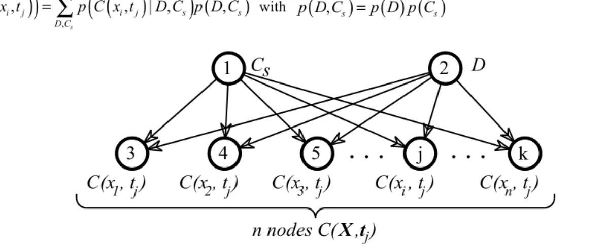
The chloride ingress could be modelled by the BN described in Figure 2 where Cs and D are the two parent nodes

(random variables to identify) labelled number 1 and 2. There are n child nodes C(xi, tj) representing the chloride

concentration at depth xi and at inspection time tj labelled number from 3 to k. The number of child nodes is computed

as:

x t

n n n

=

(6)

where nx is the total number of points in depth and nt is the total number of inspection times. Assuming that Cs and

D are two independent random variables, the values of C(xi, tj) could be easily estimated from Eq. (3). In this BN, the

probability of chloride concentration p(C(xi, tj)) can be calculated as follows (Bastidas-Arteaga, Schoefs, and Bonnet

2012; Nguyen 2007):

( )

(

)

(

( )

)

(

)

,

,

,

| ,

,

s i j i j s s D C

p C x t

=

∑

p C x t

D C p D C

with

p D C

(

,

s

) ( ) ( )

=

p D p C

s (7)

Figure 2: The BN modeling chloride ingress

To estimate p(C(xi,tj)), the conditional probability p(C(xi,tj)|D,Cs) must be already known in Eq.(7). This conditional

probability accounts for the dependence between the chloride content C(xi,tj) with the two model parameters (D and Cs)

and it is computed based on the Conditional Probability Table (CPT) of the BN. The BN allows entering evidences into the network and then updating the probabilities in the network. In this study, the evidences correspond to measures of

chloride concentration at given points and times. Then, the term p(C(xi,tj)|o) represents the probability distribution of

C(xi,tj) given evidence o and a posterior distribution can be computed by applying the Bayes’ theorem:

(

|

)

(

|

(

i, j

)

)

(

(

i, j

)

|

)

p D o =p D C x t p C x t o with

(

( )

)

(

( )

)

( )

( )

(

, |

)

| , , i j i j i j p C x t D p D p D C x t p C x t = (8) and:

(

_s|

)

(

_s|

( )

_i, _j

)

(

( )

_i, _j |

)

p C o =p C C x t p C x t o with

(

( )

)

(

( )

)

( )

( )

(

)

, | | , , i j s s s i j i j p C x t C p C p C C x t p C x t = (9)

1

Cs

2

D

3

C(x , t )

₁

4

C(x , t )

₂

5

C(x , t )

₃

j

C(x , t )

_i

k

C(x , t )

_n

. . .

. . .

n nodes C(X ,t )

j j j j j j

The determination of these conditional probabilities are carried out by the BN Tool Box which is built on the Matlab® Software.

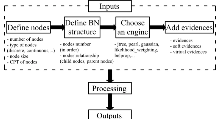
2.2.4. Parameter identification using BN built on Bayesian Network Toolbox

The Bayesian Network Toolbox (BNT) is an open-source Matlab package for directed graphical models. This can

be seen as a robust characteristic of BNT as compared with other tools because users can add, modify or make complements of functions in order to fit with the different using purposes. BNT supports many types of conditional probability distributions (nodes), many inference algorithms (exact and approximate) for both static BNs and dynamic BNs parameters and structure learning (Murphy 2001). However, BNT is a non-graphical interface environment, thus, in order to have a clear view of building a BN, we can follow the stages described in Figure 3.

We aim at identifying Cs and D from chloride profiles. To avoid hypothesis about priori information (type of

distribution, mean, standard deviation, etc.), we suppose that Cs and D follow uniform distributions in given intervals.

The interval for each parameter should contain all possible values and can be defined on the basis of existing databases, similar study cases, or expert knowledge. The assumption of uniform distribution for unknown parameter could avoid making any assumption about distribution shape (Bastidas-Arteaga, Schoefs, and Bonnet 2012; Cao and Wang 2014). Most of parameters in chloride ingress are defined in continuous space. However in order to avoid using approximate inference algorithms which will be a disadvantage when working with continuous variables, continuous variables must be replaced by discrete random variables (Straub 2009). The discretization of each parameter is described in Table 1. A

sufficient random number of Cs and D is generated and afterwards they are used to compute the chloride concentration

at depth x and time t by using Eq. (3). These priori data are used to compute the CPT for each child node in the BN. Data from inspections will be introduced to the BN as evidences. This data could be obtained both from experimental measurements or expert knowledge. In this study, for the purpose of generalization the optimization, the numerical evidences obtained from known input random variables will be generated with a sufficient number of

simulations. The probability that C(xi,tj) belongs to a given interval for different depth is then computed for the

identification of the term p(C(xi,tj)|o). These probabilities are then added to the BN as soft evidences for inference. In

this process, the BN will calculate the posterior distributions: p(Cs|o) and p(D|o) by using equations (8) and (9).

Figure 3: Flowchart of building BN on BNT Table 1: Discretization of parameters

Parameters Number of intervals Priori distribution Range

Cs (kg/m3) 16 Uniform (0.5; 8)

D (m/s²) 20 Uniform (6e-13; 3e-12)

C(xi,tj) (kg/m3) - - (0 ; 8)

In this study, numerical evidences were generated using Monte Carlo methods with parameters given in Table 2. The mean values for each parameter were taken from (Bastidas-Arteaga et al. 2009). However, the COV for each

parameter were reduced to 20% and 15% for Cs and D, respectively. This is due to the fact that within one type of

concrete, the variation was narrowed (Duracrete 2000; Vu and Stewart 2000). The assumption that Cs and D follow

lognormal distributions is also in agreement with some other researches (Duracrete 2000; Vu and Stewart 2000). These

assumptions were used to generate 10000 random values for Cs and D corresponding to 10000 independent inspections

points. This data will be served for all configurations to ensure that we used the same information to update the BN.

Inputs

Define nodes

Define BN

_structure

_{an engine}

Choose

Add evidences

- number of nodes - type of nodes (discrete, continuous,...) - node size - CPT of nodes - nodes number (in order) - nodes relationship (child nodes, parent nodes)

- jtree, pearl, gaussian, likelihood_weighting, belprop,... - evidences - soft evidences - virtual evidences

Processing

Outputs

Afterwards, each set values of C and _s D was used to compute the chloride profiles from Eq. (3). The evidences using in BN are then computed from these chloride profiles. In the final part of the paper we focus in a case in which the information is limited.

Table 2: Theoretical values of parameters to identify

Parameters Distribution Mean COV Standard deviation

Cs Lognormal 2.95 (kg/m²) 20% 0.59

D Lognormal 1.33e-12 (m/s) 15% 0.2e-12

3. SELECTION OF CONFIGURATION IN BAYESIAN NETWORK

In this section, different configurations of the BN corresponding to different inspection schemes will be analysed for selecting inspection schemes that provide the best estimation for parameters. Each configuration will be evaluated

by the error of the identified parameter Zidentified with respect to the theoretical value Ztheory as:

( )

identified theory.100% theory Z Z Error Z Z − = (10)

where Z represents the mean or the standard deviation of the parameter to identify.

3.1. Identification using one point in depth of inspection

In this part, the estimation of the chloride surface concentration (Cs) and chloride diffusion coefficient (D) will be

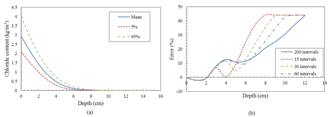
analysed from evidences obtained at one depth point. Figure 4a shows the chloride profile computed from Eq. (3) where

Cs and D have the values as shown in Table 2 at an inspection time tins = 10 years. The total inspection depth is assumed

at 12cm. At deeper point, the chloride content is almost zero. The BN now consists of three nodes: two parent nodes are

Cs and D, one child node C(xi,tj) representing for chloride concentration at depth xi and time tins = tj=10 years.

Consequently, we have 13 different BNs corresponding to 13 points in depth varying from 0cm to 12cm.

3.1.1. The convergence of the BN with the number of intervals

As previously mentioned in 2.2.4, continuous variables need to be discretised into equivalent intervals. The number of intervals could be adjusted to obtain the balance between accuracy of results and speed of computations. When a more accurate result is expected, a high value of number of intervals is often chosen. Figure 4b describes the

estimations of the error of the mean value of Cs with different discretisation and inspection depths. It is clear that, no

fluctuation is recorded in the case in which each node C(xi,tj) in the BN is divided into 200 intervals. This means that a

high number of intervals could lead to a convergence in BN. Consequently, we will keep 200 intervals for node C(xi,tj)

for all BNs in this part. This numerical implementation can be seen as a suboptimal for the estimation.

3.1.2. Analysis of the results

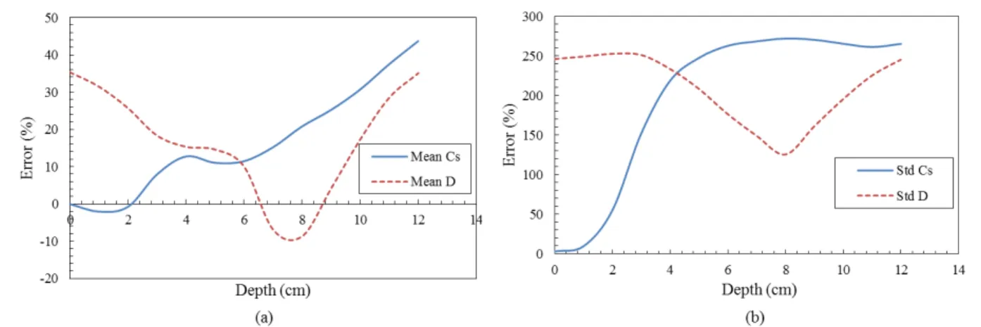
Figure 5 show the error in the identification of the mean and standard deviation of Cs and D. For Cs, the evolution of

the error of both mean and standard increases with the depth. These estimations are corresponding to the evolution of the chloride profile in Figure 4a where the chloride content reduce as depth increasing. This means that, data from chloride profiles near the surface will provide more information for the updating, whereas less information in the deeper parts increase the error in the identification. When the chloride content is closed to zero, these errors will reach the highest value that are close to 40% for the mean. On the contrary, with the evidences near the surface (x ≈ 0), we can

obtain the best estimation for the mean and standard deviation of Cs, with errors are 1% and 3% respectively. This

might due to the fact that in Eq. (3), when we set x ≈ 0, C(xi,tj) ≈ Cs. Consequently, the chloride concentration at the

surface is most valuable in the identification of C and the BN will put more weight on the evidence obtained at x = 0 _s

cm.

It is also observed in Figure 5 that the error in the identification of D decreases when the depth x < 8cm and after increases. This behaviour corresponds to the fact that chloride content at deeper parts is more useful in predicting the

diffusion coefficient. However, at deep points where the chloride contents are close to zero for tins =10yr, the error will

increase. The errors in the identification of the standard deviation of D followed a similar trend, however their values are very far from the theoretical values with important errors (more than 200%). Therefore, it can be concluded that it is impossible to perform a good identification of D using evidences obtained from only one point in depth.

3.2. Identification using full inspection depth

3.2.1. Using the same boundary for all the child nodes

In this section, the identification in BN will use data from total inspection depth. The total inspection depth (12cm) is divided into intervals to select several points for updating the BNs. The intervals length should not be smaller than 0.3cm due to the accuracy of the equipment for determining chloride profiles. The BNs will now have the number of child nodes equal to the number of measurements in depth. Table 3 presents the different cases considered in this part.

Table 3: Different discretization cases and number of points in depth

Case _(cm) Δx Discretization Number of points _{in depth} 1 0.3 0:0.3:12 41 2 0.5 0:0.5:12 25 3 1 0:1:12 13 4 2 0:2:12 7 5 3 0:3:12 5

Figure 6 presents the error in the identification using full inspection depth and the same boundaries for the child

nodes. It is noted that there is no remarkable change in the identification of the mean of Cs (Figure 6a) because the

errors in 5 surveyed cases are under estimated at approximate -5%. Meanwhile it seems that increasing the number of

measurements in the inspection depth might produce more errors for the standard deviation of Cs (Figure 6b).

Interestingly, the gap between identified values and theoretical values for D are reduced significantly when the size of the discretization intervals is smaller. The errors in the estimation of the mean of D are less than 5% when the intervals are smaller than 0.5 cm. The standard deviation of D also reveals a better evolution when the error decreases from more

than 200% with Δ =x 3cm _{to about 20% with} Δ =x 0.3cm. This behaviour is expected because when the inspection depth is divided into small intervals, we could obtain more information describing the level of chloride ingress that is useful for characterizing the diffusion coefficient. Hence, data from full inspection depth could be more useful in the identification of D.

3.2.2. Using different boundaries for child nodes

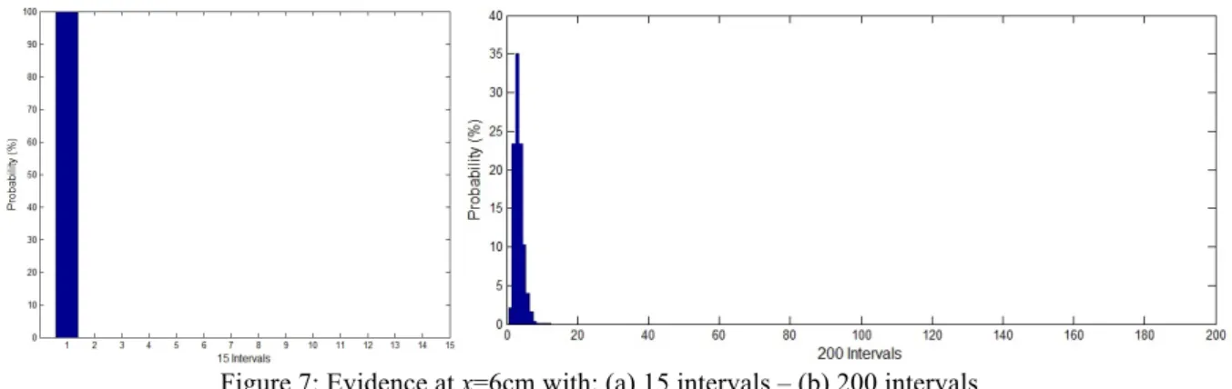
As discussed in section 3.2.1., when the inspection depth is divided into large intervals, the errors in the estimation of chloride diffusion coefficient increase significantly. This is because, when the number of measured points decreases, the information used to update the BN becomes poor, making that the chloride content in deeper points become more important for predicting the level of chloride ingress. However, the chloride levels in deeper parts are low and if the number of intervals is not large enough, the discretization will not be able to give a good assessment of the probability to build the evidences. For example, in Figure 7a, the evidence at depth x = 6cm with 15 intervals does not provide a good information for updating the probability of the BN. Consequently, a high value for the number of intervals will be required to obtain a better estimation (Figure 7b). Nevertheless, increasing the number of intervals will increase the size of the CPTs, which might also increase the computational time for the BN.

Figure 7: Evidence at x=6cm with: (a) 15 intervals – (b) 200 intervals

In this section, a proposed algorithm to optimize the information used in BN is investigated. The number of intervals in the discretization is remained at a low value to reduce the computational time. However, we did not used the same

range of discretisation for all child nodes C(xi,tj). Each node C(xi,tj) was corresponding to a specific range which is

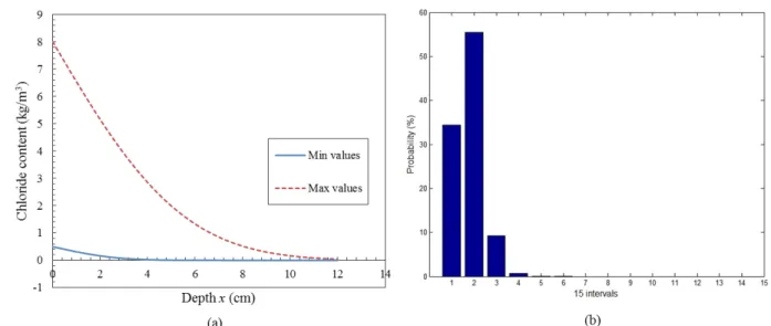
defined by the min and the max value of the chloride concentration at depth x from the priori data (Figure 8a).By this means, we can optimize the information in deep points for building the evidences. Figure 8b shows the evidence at depth x= 6cm with 15 intervals and the range is defined for each node in BN. It is clear that the evidence at depth x=

6cm now could provide more information for updating the probability of the BN in this case.

Figure 8: (a) The range for each node at depth x – (b) Evidence at x= 6cm with 15 intervals and different range Figure 9 shows the comparison in the estimation of the mean and standard deviation of D. It is clear that, in both cases: using a large number of intervals and using different ranges, the errors are reduced remarkably despite of the inspection length was divided into large intervals. This proposed approach could be very useful in practice when the number of measured points is limited or when the chloride content penetrated into concrete is low.

3.2.3. Using evidences from different inspection times

In this section, evidences obtained from various inspection times will be introduced in the BN for the identification process. According to section 3.2.2, various boundaries were used for each child node in the BN with a sufficient number of intervals to minimize the fluctuation effects/errors in the results.

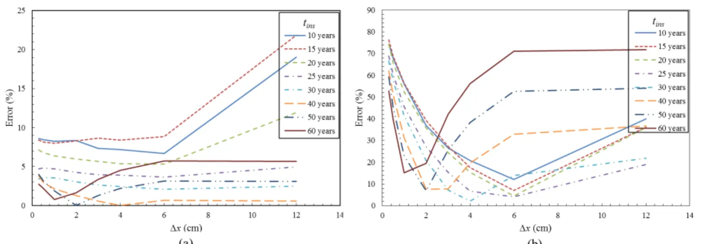
From Figure 10, it can be seen that the inspection time tins influences the estimation of both the mean and standard

deviation of D. The identification is improved when tins increases until arriving at an optimal inspection value tins,opt that

varies between 30 and 40 years for the identification of the mean and standard deviation. This phenomenon can be

explained by the fact that when tins ≈ 35 years the chloride concentration in the total inspection length is sufficient for

describing the chloride ingress process – i.e. there is sufficient chloride content at each point in the space to improve the

identification. When tins > 40 years, the chloride content at x = 12 cm is larger that zero and therefore the identification

errors increase because the inspection length is not enough larger to describe the problem.

It is also worth noticing that there is an optimal value Δxopt for each inspection time. The optimum value decreases

when tins increases. This is related to the fact that for larger tins the chloride content inside the total inspection length is

larger. Consequently, it is necessary to add more information to improve the representation of the chloride profile. It is

also noted that the error is larger for smaller values of Δx in comparison with the Δxopt. There is no remarkable change

in the estimation the mean value of D when ∆x vary from 0.3 cm to the optimal value. However, the variation is more important for the identification of the standard deviation of D. This is mainly related to size of Δx as described in Figure 11. When ∆x is small, the chloride content is almost the same between the two adjacent inspection points. Therefore, the probability densities of the evidences used for updating in BN are very similar for two adjacent inspection points:

x=0cm and x=0.3cm (Figure 11a). This will increases the errors in estimating the mean and standard deviation when

using close points. In contrast, when ∆x increase (x=0cm and x=2cm), the probability densities of the evidences will be more different by reducing the identification errors (Figure 11b). When ∆x is larger than the optimal value, the errors for both mean and standard deviation increase because the information becomes poor for describing the chloride ingress process.

Figure 10: Error estimation for D with evidences from different inspection times: (a) The Mean - (b) The standard deviation

Figure 11: Effect of the discretization on the error of standard deviation: (a) with ∆x=0.3 cm – (b) with ∆x=2 cm

For Cs, the results presented in Figure 12 reveal that to obtain a good estimation of Cs, it is better to use the

evidences at early inspection times. This is because the chloride surface concentration does not depend on the time of inspection and at early inspections times the chloride concentration in the neighbouring of the concrete surface will be

close to Cs. The results also show that using more points in depth improve significantly the assessment of the standard

deviation because there is more information available.

Figure 12: Error estimation for Cs with evidences from different inspection times: (a) The Mean - (b) The standard

4. Assessment the probability of corrosion initiation

This section examines the influence of the identified data identified from BN on the evaluation of the probability of

corrosion initiation for tins = 10years. For estimating this probability, we considered that the threshold of chloride

concentration for the initiation of corrosion follows an uniform distribution -

Cth= U µ = 0.9kg / m

3_{;σ = 0.2kg / m}3

(

)

(Vu and Stewart 2000) and the cover depth of reinforced bar is 6 cm. The histograms obtained after updating the BN for each parameter will be used directly in Monte Carlo simulations to estimate the probability of corrosion initiation to avoid any assumption about analytical distribution laws.

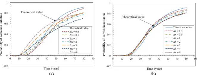
Figure 13a shows that, data identified from one depth point (section 3.1) does not provide an acceptable prediction of the probability of corrosion initiation in comparison with the theoretical data. However, from Figure 13b, it is noted that the prediction of the probability of corrosion initiation from data identified from several inspection points (section 3.2) is more close to the theoretical values. The error is reduced when Δx is smaller.

The results presented above considered a large number of simulations for the generation of numerical evidences. However, in real practice, the number of profiles collected after an inspection campaign is very limited. Figure 14 presents the probability of corrosion initiation estimate with limited data. In this case, the numerical evidences were generated from 15 profiles of chloride content obtained from Monte Carlo simulation. Figure 14a describes the results obtained by considering the full inspection length that minimised the errors according to Figure 13b. However, it is noted that the assessment of the probability of corrosion initiation is far of the theoretical values even for small values of Δx. In this situation, it is necessary to optimize the information used for updating the BN. To improve the identification, we combine results of one point inspection and several point inspections. We use therefore the results of

the identification of Cs obtained with one depth point (x ≈ 0) as a priori data for the estimation of D by considering the

full depth. The results of probability of corrosion initiation comparing these two cases: before optimization and after optimization are shown in Figure 14. It is clear that this strategy improves the identification when data is limited. It could be concluded that this approach would be very useful for limited data. The assessment could be improved if we consider data of other inspection times (section 3.2.3).

Figure 13: Probability of corrosion initiation with data obtained: (a) from single point inspection depth - (b) from full inspection depth

5. CONCLUSIONS

The penetration of chloride is one of the main causes inducing corrosion of RC structures. The identification of parameters in chloride ingress modelling is crucial in predicting chloride ingress into concrete that will help to optimise the maintenance of structures exposed to chloride-contaminated environments. Inspection data used for the identification is very limited due to time-consuming and expensive tests. Therefore, it is necessary to use these data in an optimal scheme. Within this framework, the BN could provide a possibility to identify model parameters with different information. In this study, results based on numerical evidences revealed that there are optimal configurations

of BN for the identification of each parameter (Cs or D). For Cs, an early inspection with one point close to the surface

could provide a good identification. For D, to obtain identified values close to the theoretical values, the identification should use the evidences from full inspection depth. At a specific inspection time, there is an optimal discretization for the inspection length that could provide the best estimation for D. These optimal configurations could be combined to improve the identification of the model parameters. An application to the assessment of the probability of corrosion initiation showed that the approach is useful even if information is limited.

Further work in this area will focus on

• the consideration of information obtained at different points in time, • the use of real data, and

• the consideration of more complete deterioration models. 6. REFERENCES

Bastidas-Arteaga, E., Ph. Bressolette, A. Chateauneuf, and M. Sánchez-Silva. 2009. “Probabilistic Lifetime Assessment of RC Structures under Coupled Corrosion–fatigue Deterioration Processes.” Structural Safety 31(1): 84–96. Bastidas-Arteaga, E., A. Chateauneuf, M. Sánchez-Silva, Ph. Bressolette, and F. Schoefs. 2011. “A Comprehensive

Probabilistic Model of Chloride Ingress in Unsaturated Concrete.” Engineering Structures 33: 720–30.

Bastidas-Arteaga, E., and F. Schoefs. 2012. “Stochastic Improvement of Inspection and Maintenance of Corroding Reinforced Concrete Structures Placed in Unsaturated Environments.” Engineering Structures 41: 50–62.

Bastidas-Arteaga, E., F. Schoefs, and S. Bonnet. 2012. “Bayesian Identification of Uncertainties in Chloride Ingress Modeling into Reinforced Concrete Structures.” In Third International Symposium on Life-Cycle Civil Engineering, Vienna, Austria.

Bonnet, S., F. Schoefs, J. Ricardo, and M. Salta. 2009. “Effect of Error Measurements of Chloride Profiles on Reliability Assessment.” In 10th International Conference on Structural Safety and Reliability, eds. H Furuta, D M Frangopol, and M Shinozuka. Osaka, Japan.

Cao, Z., and Y. Wang. 2014. “Bayesian Model Comparison and Selection of Spatial Correlation Functions for Soil Parameters.” Structural Safety.

Duracrete. 2000. Probabilistic Calculations. DuraCrete—probabilistic Performance Based Durability Design of Concrete Structures. EU—brite EuRam III. Contract BRPR-CT95-0132. Project BE95-1347/R12-13.

Murphy, K.P. 2001. “The Bayes Net Toolbox for Matlab.”

Nguyen, X.S. 2007. “Algorithmes Probabilistes Appliqués À La Mécanique Des Ouvrages de Génie Civil.” PhD Thesis, INSA de Toulouse.

Richard, B., L. Adelaide, and C. Cremona. 2012. “A Bayesian Approach to Estimate Material Properties from Global Statistical Data.” European Journal of Environmental and Civil Engineering (March 2013): 37–41.

Rosquoët, F., S. Bonnet, F. Schoefs, and A. Khelidj. 2006. “Chloride Propagation in Concrete Harbor.” In 2nd International RILEM Symposium on Advances in Concrete through Science and Engineering, eds. J Marchand, B Bissonnette, R Gagne, M Jolin, and F Paradis. Quebec, Canada: RILEM Publications.

Saassouh, B., and Z. Lounis. 2012. “Probabilistic Modeling of Chloride-Induced Corrosion in Concrete Structures Using First- and Second-Order Reliability Methods.” Cement and Concrete Composites 34(9): 1082–93.

Straub, D. 2009. “Stochastic Modeling of Deterioration Processes through Dynamic Bayesian Networks.” (October): 1089–99.

Tuutti, K. 1982. “Corrosion of Steel in Concrete.” Swedish Cement and Concrete Institute.

Vu, K.A.T., and M.G. Stewart. 2000. “Structural Reliability of Concrete Bridges Including Improved Chloride-Induced Corrosion.” Structural Safety 22: 313–33.

RESPONSIBILITY NOTICE