Risk-Based-Optimization of Geo-positioning of Sensors in Case of Spatial Fields of Deterioration/Properties

HAL Id: hal-01008854

https://hal.archives-ouvertes.fr/hal-01008854

Submitted on 19 May 2018

HAL is a multi-disciplinary open access archive for the deposit and dissemination of sci-entific research documents, whether they are pub-lished or not. The documents may come from teaching and research institutions in France or abroad, or from public or private research centers.

L’archive ouverte pluridisciplinaire HAL, est destinée au dépôt et à la diffusion de documents scientifiques de niveau recherche, publiés ou non, émanant des établissements d’enseignement et de recherche français ou étrangers, des laboratoires publics ou privés.

Risk-Based-Optimization of Geo-positioning of Sensors

in Case of Spatial Fields of Deterioration/Properties

Trung-Viet Tran, Franck Schoefs, Emilio Bastidas-Arteaga

To cite this version:

Trung-Viet Tran, Franck Schoefs, Emilio Bastidas-Arteaga. Risk-Based-Optimization of Geo-positioning of Sensors in Case of Spatial Fields of Deterioration/Properties. ICOSSAR’11, 2013, New York, United States. �10.1016/j.engstruct.2017.08.070�. �hal-01008854�

1 INTRODUCTION

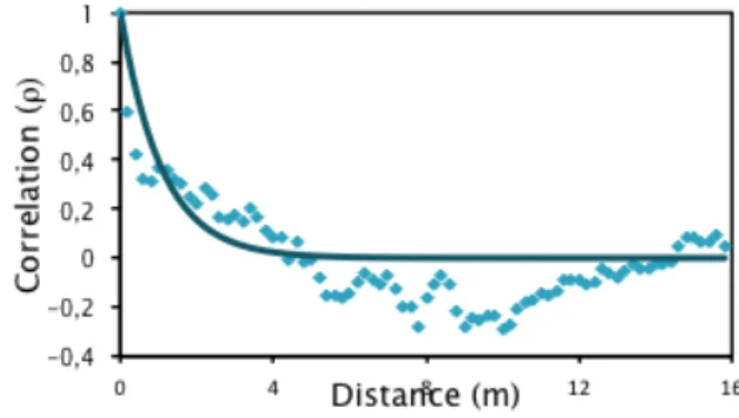
The localization of weak properties or bad behavior of a structure is still a challenge for Structural Health Monitoring (SHM) design (Okasha and Frangopol, 2012). In case of random loading or material proper-ties, this challenge is arduous because of the limited number of sensors and the quasi-infinite potential positions of local failures. Deterministic algorithms and specific multi-sensors systems are developed to this aim. In that case, generally, the precision of the positioning of a defect goes with a lack of sizing. However, the stochastic field is rarely a pure white noise and has a stochastic structure and probabilistic properties. These properties should be used to pro-vide rational aid tools for optimizing the number of sensor. The paper shows that the stationary property is sufficient to find the optimal quantity of sensors and their position in view to assess accurately the shape of the auto-correlation function (see Fig. 1) that guides the position of control through Non De-structive Techniques (NDT) during the service life. If we focus on embedded sensors, these stochastic properties are less sensitive to environmental condi-tions (sun, humidity, …) at the surface of the struc-tures where usual NDT tools are affected by. That will help the help the planning of NDT campaigns. The evolution of measurement with time is out of the scope of the present paper.

The paper starts with key concepts and illustra-tion of spatial random field modeling.

In the next section, a method for optimal sensor positioning is suggested by focusing on the assess-ment of the correlation function. The quality is

ex-pressed in terms of confidence interval on the pa-rameters of the auto-correlation function.

Figure 1. Auto-correlation function fitted with a parametric function.

2 SPATIAL RANDOM FIELD MODELLING 2.1 Usual approaches for spatial field modeling

The stochastic field could take several forms more or less complicated. The most simple when the deg-radation can be considered as homogeneous is the stationary stochastic field that can be used, for in-stance, to model chloride distribution (O’Connor & Kenshel 2013), concrete properties (Bazant, 1991; 2000a; 2000b) or soil properties. In some cases, when a stochastic process is influenced by several phenomena that vary with time (sea wave for in-stance) or with space (concreting of a structure in several steps with heterogeneity of these steps), it can be modeled as piecewise stationary. This more sophisticated stochastic field can represent, for

ex-Risk-Based-optimization of geo-positioning of sensors in case of spatial

fields of deterioration/properties

T.V. Tran, F. Schoefs, E. Bastidas-Arteaga

LUNAM Université, Université de Nantes, Institute for Research in Civil and Mechanical Engineering, CNRS

ABSTRACT: The localization of weak properties or bad behavior of a structure is still a very challenging task that concentrates the improvement of Non Destructive Testing (NDT) tools on more efficiency and higher structural coverage. In case of random loading or material properties, this challenge is arduous because of the limited number of measures and the quasi-infinite potential positions of local failures. The paper shows that the stationary property is useful to find the minimum quantity of NDT measurements and their position for a given quality assessment. A two stages procedure allows us (i) to quantify the properties of the ergodic, sta-tionary field (ii) to assess the distribution of the characteristics. The paper focuses on optimization of sensor geo-positioning to reach (i): the criterion relies on the width of the confidence interval. The concept of critical upper bound spatial correlation is introduced.

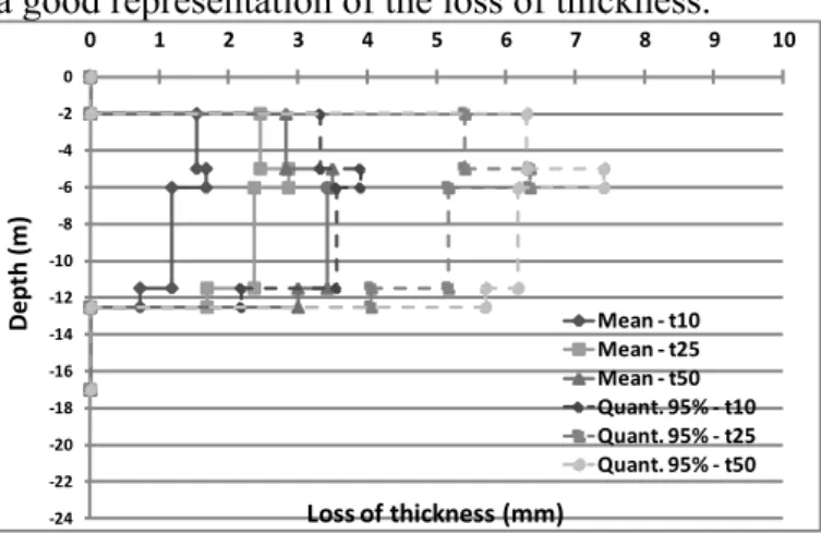
ample, the variability of concreting materials by pieces or the corrosion of structures located in con-tiguous environments with different characteristics (Boéro et al 2009, 2012). That is the case for the cor-rosion of sheet-piles in marine environment where the corrosion process is governed by several phe-nomena that depend on the exposure zone E. For il-lustrating this case, Figure 2 presents the spatial var-iability of the mean and the 95% quantiles of steel thickness loss in different zones at 10, 25 and 50 years (t10, t25 and t50. It can be observed that both the mean and the 95% quantile are well defined for the considered zones –i.e., E∈[EA, ET, EL, EI, EM, ES] limited by dashed lines: from the top to the bottom, Aerial (A), Tide (T), Low level of tide (L), Immer-sion (I), Mud (M) and Soil (S). In this case, a piece-wise stationary stochastic field could be used to have a good representation of the loss of thickness.

-­‐24 -­‐22 -­‐20 -­‐18 -­‐16 -­‐14 -­‐12 -­‐10 -­‐8 -­‐6 -­‐4 -­‐2 0 0 1 2 3 4 5 6 7 8 9 10 D ep th  (m )

Loss  of  thickness  (mm)

Mean  -­‐ t10 Mean  -­‐ t25 Mean  -­‐ t50 Quant.  95%  -­‐ t10 Quant.  95%  -­‐ t25 Quant.  95%  -­‐ t50

Figure 2. Mean value and 95% quantiles of steel thickness loss in each zone at time 10, 25 and 50 years.

2.2 Usual approaches for inspection modeling During measurement, there are many factors that in-fluence the quality of measurements –e.g, environ-mental conditions, error in the placement of the sen-sor, error due to sensor and error induced by the op-erator (Bonnet et al. unpubl., Breysse et al. 2009). These factors could lead, for a given measurement, to under or overestimations of the measured parame-ter. If the parameter is underestimated and the owner could decide, “do nothing” when repair is required. On the contrary, an overestimation generates a “wrong decision” where the early repair generates overcharges (Rouhan & Schoefs 2003, Sheils et al. 2012). In this paper we will consider inspection as perfect: that (i) there is no bias, (ii) error is ble or redundancy allows us to assume it as negligi-ble.

2.3 Main assumptions for the stochastic modeling Starting from the previous sections and to limit the study, we consider five main assumptions about the sensor and the random field modeling.

- The stochastic field is statically homogeneous, and only few information on the marginal dis-tribution is known: the type of the unique

probability density distribution. In the follow-ing applications we consider a Gaussian field; - A limited number (from 30 to 50) of discrete

sensors can be placed;

- Second order stationary stochastic field can piecewise or totally describe the spatial fields; - Sensors are considered as perfect as defined by

Schoefs et al. (2009).

Given a probability space (Ω, F , P), a stochastic

field or process with state space Z is a collection of

Z-valued random variables indexed respectively by a

set s “space” or t “time”. Let us denote Z(x, θ) the one-dimensional stochastic field where θ represents the randomness and x the spatial coordinate.

Z(x,θi) is called the ith trajectory of this field and

corresponds to a given realization θi of the field for whatever location. Z(x1, θ) is a random variable that is generated by θ at a given location x = x1. We con-sider here homogeneous fields only. This means that the marginal distribution of Z(x1, θ) does not depend on the location.

A stochastic field is second order stationary if it fol-lows three main properties:

• expectation E[Z(x, θ)] does not depend on the

lo-cation x –i.e., E[Z(x, θ)] = E[Z];

• variance V[Z(x, θ)] does not depend on the

loca-tion x –i.e., V[Z(x, θ)] = V[Z]; and

• spatial covariance COV[Z(x, θ), Z(x, θ)] depends

only on the distance (x-x’).

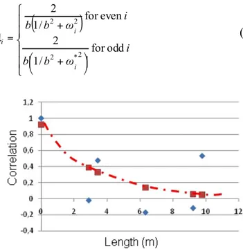
Thus, the second order stationary is a property re-stricted to the two first probabilistic moments. It can be shown that geometries of welds for ships or the spatial distribution of chloride concentration in rein-forced concrete structures can be represented by sta-tionary stochastic fields (Schoefs et al. 2011a). For instance, Figure 3 presents the correlation function of the chloride diffusion coefficient as function of the distance between two points (duratiNet project: http://www.duratinet.org, following O’Connor & Kenshel 2013). Note that if E[Z(x, θ)] is not constant with space, the signal can be centered and the prop-erties been proved for the field (Z(x, θ) – E[Z(x, θ)]). Several approaches can be used to represent a stochastic field Z(x, θ): Karhunen-Loève expansion, approximation by Fourier series, and approximation EOLE (Li & Der Kiureghian 1993). In this paper, we select a Karhunen-Loève expansion to represent the stochastic field of resistance of a structure

Z(x, θ). This expansion represents a random field as

a combination of orthogonal functions on a bounded interval [–a, a]:

Z(x,θ ) = µZ+σZ. λi.ξi(θ ).

i=1 n

∑

where, µZ is the mean of the field Z, σZ is the stand-ard deviation of the statistically homogeneous field

Z, n is number of terms in the expansion,

ξ

of centered Gaussian random variables and

λ

are, respectively, the eigenvalues and eigen func-tions of the correlation function ρ(Δx). It is possible

to analytically determine the eigenvalues λi and eig-en functions fi for some correlation functions (Ghanem & Spanos 2003). For example, it can be determined if we assume that the field is second or-der stationary and we use an exponential correlation function (Vanmarcke, 1983):

ρ(Δx = x1- x2)=exp( − Δx

b ); 0 < b

(2) where b is the correlation length and Δx ∈ [–a, a]. Accounting for the stationarity of the process, the following transcendental equations can be obtained:

1 b−ω tan(ωa) = 0 ω −1 btan(ωa) = 0 " # $ $ % $ $ (3)

where ω is obtained by solving equation (3). If the solution of the second equation is noted ω*, the ei-genfunctions are: ⎪ ⎪ ⎩ ⎪ ⎪ ⎨ ⎧ − + = i ω a ω a x ω i ω a ω a x ω x f i i i i i i i odd for 2 / ) 2 sin( ) sin( even for 2 / ) 2 sin( ) cos( ) ( * * * (4)

and the corresponding eigenvalues are:

(

)

Figure 3. Spatial correlation of the chloride diffusion coeffi-cient in concrete – data Trinity College of Dublin.

3 SENSOR POSITIONNING STRATEGY AND GOALS

3.1 Key ideas for sensor geo-positioning

The paper focuses on the assessment of the auto-correlation function of a stationary field. An optimal geo-positioning of sensors along a trajectory (Fig. 4) should give an accurate value of the parameters (i.e.

b) with a limited number of sensors.

x(m)

?Lb ?Lb

Z

Ns (measurements)

Figure 4. Non-regularly spaced sensors along a trajectory.

When looking to the usual shape of a correlation function (Fig.1) a regular spacing ‘Lb = a’ of Ns sen-sors appears not optimal: it provides a dense infor-mation for distances ‘a, 2a, … (Ns-1)a’ but none be-tween. We get a non-homogeneous quantity of data:

Ns for distance 0, (Ns-i) for distance ia (1<i< Ns). The objective will be to get a spacing of sensor that leads to a more homogeneous quantity of data in the zone f high correlation as defined on Figure 5. Moreover, there is a limited feed-back on the auto-correlation length on site and the uncertainty on the value of ‘b’ (Eq. 2) when installing the sensors is significant. A ut o-c orre la ti on ( ρ ) 1

Fitted auto -corrélation function ( parameter b)

x (m) Mesurement

High correlation zone

L_m ? Nc ?

Figure 5. High correlation zone and homogeneous measure-ments long the trajectory.

These reasons lead us to suggest a non-regular spacing of the sensors.

3.2 Definition of the Spatial Correlation Threshold The When the uncertainty of the should of an stages inspection we suggest should provide both the parameters of the spatial correlation function and in-dependent events that characterize the marginal dis-tribution of Z. We considerer in this paper a one-dimensional spatial field and we will apply the methodology on a set of trajectories: these

trajecto-ries could be a set of 1D components (beams), or a very long 1D-component subdivided artificially or physically (expansion joint or construction joints) in a set of short components, or belong to a wall struc-ture (steel sheet pile or concrete wall).

In view to limit the costs of the monitoring (num-ber of sensor) we inspect a trajectory with a “suffi-ciently low distance Lb” to assess the shape of the correlation function (2): for instance the shape pa-rameter b. This “sufficiently low” can be seen as an Inspection Distance Threshold (ICD). Thus the non regular distances of sensor spacing Lbi should satis-fy: Lbi ∈ ]0, IDT[ where L is the length of the trajec-tory.

For illustrating the methodology, we consider in the following a set of 1D-components (beams) with infinite length L ~ ∞: we don’t discuss the case of components with a limited size, especially those where L< Lb for which it is quite impossible to char-acterize the spatial variability. The IDT is defined by assuming that after a given distance, the events measured from an inspection can be assumed as sta-tistically independent. A Spatial Correlation Thresh-old SCT of the spatial correlation gives this weak correlation. For instance in Figure 3 (red line) for SCT=0.4, IDT=3 meters. It is linked with IDT by the relationship:

IDT = b. ln(SCT ) (6)

3.3 Parameterization of the non-regular spacing In view to reduce the set of potential solutions and simplify the design of the network of sensors, we suggest a parameterization. It is based on a division of the trajectory into np pieces of same size Lm (see Fig. 6) and then a subdivision of each piece into a decreasing number of pieces of same size following a series (7). NS i ≈ NS 1i j " # " $ % $; j ∈ 1i...n

{

}

∑

Where !" #$. denotes the floor function,N_Sjis the

num-ber of sensors in the jth piece and NS

1i_{is the initial} number of sensors in the 1st piece, the final number of inspection NS

1 f _{in the first section is} computing following: NS 1 f = NS− NS j j>1

∑

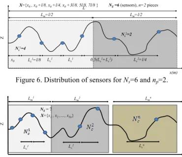
For instance, for two pieces and 6 sensors, 4 are placed in the first piece and 2 in the second (Fig. 6). Figure 7 presents the case 7 sensors and 3 pieces.

x(m) 0,5(Lc1+Lc2) Lc2=l/4 Z Lc1=l/8 x0 NS =6 (sensors), n=2 pieces Lc1 Lc1 X={x0 , x0 +l/8, x0 +l/4, x0 +3l/8, 5l/8, 7l/8 } Ns1=4 Ns2=2 L Lm=l/2 Lm=l/2

Figure 6. Distribution of sensors for Ns=6 and np=2.

x(m) Lcn Z Lc1 X={x1 , x2 ,…, xNs} NS = 7 Lc2 Lm1 Lm2 Lmn

Figure 7. Distribution of sensors for Ns=7 and np=3.

Our objective is now to optimize the number of inspections in view to reach a given quality of the result.

4 APPLICATION

4.1 Assumptions and inputs

We consider in this section a beam of length

L=25 m with a limited number of sensors Ns=30.

The objective is to optimize their position in view to reach a good assessment of b (see Eq. 2). Only one trajectory is instrumented and the uncertainty due to the stochastic field is simulated by (1) with: µZ=100

(MpA) ; σZ=20 (MPa) ; b=1m.

We analyze the error between the theoretical val-ue and the assessed one.

4.2 Results and inputs

We vary the number of pieces from 1 (30 sensors) to 6 (12, 6, 4, 3, 3, 2 sensors on each piece). Figure 8 presents plots the difference ( ˆb -b) between the es-timated value and the theoretical one (here b=1) for 1000 simulated trajectories. The regular spacing ob-tained for np=1 shows the biggest uncertainty in the assessment of b with potential errors of 0.8 (near 100%). The cutting with 6 pieces shows a systematic underestimation of b.

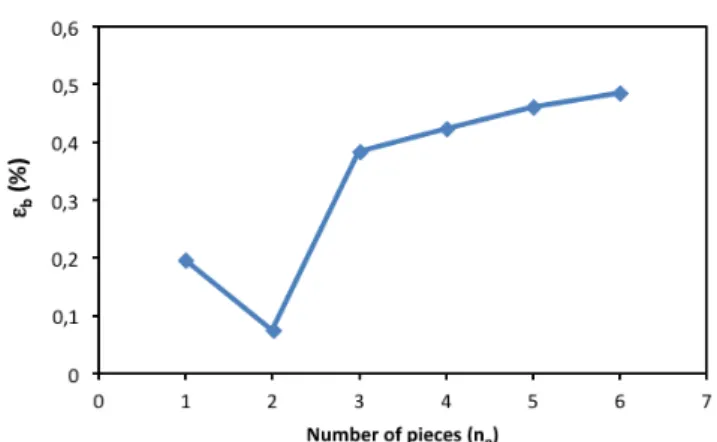
Let us focus on εb*, the normalized mean error on

b presented in Equation (9). Figure 9 gives the plot

of this error as a function of np. εb * = 1 1000 ˆ bk− b b " # $ % & ' k

∑

Figure 8. Distribution of sensors for Ns=7 and np=3.

Figure 9. Normalized error on b as a function of np.

Following this criterion, it is shown that the spac-ing with np=2 is optimal.

5 CONCLUSION

We propose in this paper an original method for the non-regular spacing of sensors devoted to the as-sessment of stationary fields from embedded sen-sors. The method is based on the uncertainty as-sessment of the parameter of the auto-correlation function. Numerical simulations of Gaussian sta-tionary stochastic illustrate the potential of the method by showing that it provides a decision aid tool when a limited number of sensors are placed in a structure.

6 AKNOWLEDGEMENTS

The authors would like to acknowledge the Pays de la Loire Region and the project ECND-PdL for their support and the duratiNet EC Interreg project (http://www.duratinet.org).

7 REFERENCES

Bazant, Z. & Novák, D. 2000a. Probabilistic Nonlocal Theory for Quasibrittle Fracture Initiation and Size Effect. I: Theo-ry. Journal of Engineering Mechanics 126(2): 166-174. Bazant, Z. & Novák, D. 2000b. Probabilistic Nonlocal Theory

for Quasibrittle Fracture Initiation and Size Effect. II: Ap-plication. Journal of Engineering Mechanics. 126(2): 175-185.

Bazant, Z. & Xi, Y. 1991. Statistical Size Effect in Quasi-brittle Structures: II. Nonlocal Theory. ASCE J. of Engrg.

Mech. 117(11): 2623-2640.

Boéro, J., Schoefs, F., Melchers, R., & Capra, B. 2009. Statisti-cal analysis of corrosion process along French coast. In proceedings of ICOSSAR’09. Paper no. 528. Mini-symposia MS15. System identification

Boéro J., Schoefs F., Yáñez-Godoy H., Capra B. 2012. Time-function reliability of harbour infrastructures from stochas-tic modelling of corrosion. European Journal of

Environ-mental and Civil Engineering, 16(10)/Nov.2012:

1187-1201.

Bonnet, S., Schoefs, F. & Salta, M. unpubl. Statistical study and probabilistic modelling of error when building chloride profiles for reliability assessment. submitted February 22th 2013.

Breysse, D., Yotte, S., Salta, M., Schoefs, F., Ricardo, J. & Chaplain M. 2009. Accounting for variability and uncer-tainties in NDT condition assessment of corroded RC-structures. European Journal of Environmental and Civil

Engineering, “Durability and maintenance in marine

envi-ronment” 13(5): 573–592.

Ghanem, R. & Spanos R.D. 2003. Stochastic Finite Elements -

A Spectral Approach. Springer, New York, USA.

Li, C. & Der Kiureghian, A. 1993. Optimal discretization of random field. Journal of Engineering Mechanics, 199: 1136-1154.

O'Connor, A., & Kenshel, O. 2013. Experimental Evaluation of the Scale of Fluctuation for Spatial Variability Modeling of Chloride-Induced Reinforced Concrete Corrosion. Journal Of Bridge Engineering 18(1)/Jan 2013: 3-14.

Okasha, N. & Frangopol, D. 2012. Integration of structural health monitoring in a system performance based life-cycle bridge management framework, Structure And

Infrastruc-ture Engineering, 8(11): 999-1016.

Rouhan A. & Schoefs F. 2003. Probabilistic modeling of in-spection results for offshore structures. Structural Safety, 25:379-399.

Schoefs, F., Clément A. & Nouy A. 2009. Assessment of spa-tially dependent ROC curves for inspection of random fields of defects. Structural Safety 31(5)/Sept. 2009: 409-419.

Schoefs, F., Yáñez-Godoy, H., Lanata, F. 2011a. Polynomial Chaos Representation for Identification of Mechanical Characteristics of Instrumented Structures: Application to a Pile Supported Wharf, Computer Aided Civil and

Infra-structure Engineering, spec. Issue “Structural Health Mon-itoring” 26(3): 173–189.

Sheils, E., O’Connor, A., Schoefs, F. & Breysse, D. 2012. In-vestigation of the Effect of the Quality of Inspection Tech-niques on the Optimal Inspection Interval for Structures,

Structure and Infrastructure Engineering: Maintenance, Management, Life-Cycle Design and performance (NSIE),

Spec. Iss. “Monitoring, Modeling and Assessment of Struc-tural Deterioration in Marine Environments” 8(6)/June 2012: 557-568.

Vanmarcke, E. 1983. Random fields: analysis and synthesis.