The Hidden Robot: an Efficient Concept Contributing to the Analysis of the Controllability of Parallel Robots in Advanced Visual Servoing Techniques

HAL Id: hal-01203183

https://hal.archives-ouvertes.fr/hal-01203183

Submitted on 24 Jun 2019

HAL is a multi-disciplinary open access

archive for the deposit and dissemination of

sci-entific research documents, whether they are

pub-lished or not. The documents may come from

teaching and research institutions in France or

abroad, or from public or private research centers.

L’archive ouverte pluridisciplinaire HAL, est

destinée au dépôt et à la diffusion de documents

scientifiques de niveau recherche, publiés ou non,

émanant des établissements d’enseignement et de

recherche français ou étrangers, des laboratoires

publics ou privés.

to the Analysis of the Controllability of Parallel Robots

in Advanced Visual Servoing Techniques

Sébastien Briot, Philippe Martinet, Victor Rosenzveig

To cite this version:

Sébastien Briot, Philippe Martinet, Victor Rosenzveig. The Hidden Robot: an Efficient Concept

Contributing to the Analysis of the Controllability of Parallel Robots in Advanced Visual Servoing

Techniques. IEEE Transactions on Robotics, Institute of Electrical and Electronics Engineers (IEEE),

2015, 31 (6), pp.1337-1352. �hal-01203183�

The Hidden Robot: an Efficient Concept

Contributing to the Analysis of the Controllability

of Parallel Robots in Advanced Visual Servoing

Techniques

S´ebastien Briot, Philippe Martinet, and Victor Rosenzveig

Abstract—Previous works on parallel robots have shown that their visual servoing using the observation of their leg directions was possible. There were however found two main results for which no answer was given. These results were that (i) the observed robot which is composed of n legs could be controlled in most cases using the observation of only m leg directions (m < n), and that (ii) in some cases, the robot did not converge to the desired end-effector pose, even if the observed leg directions did (i.e. there was not a global diffeomorphism between the observation space and the robot space).

Recently, it was shown that the visual servoing of the leg direc-tions of the Gough-Stewart platform and the Adept Quattro was equivalent to controlling other virtual robots that have assembly modes and singular configurations different from those of the real ones. These hidden robot models are tangible visualizations of the mapping between the observation space and the real robots Cartesian space. Thanks to this concept, all the aforementioned points pertaining to the studied robots were answered.

In this paper, the concept of the hidden robot model is generalized for any type of parallel robots controlled using visual servos based on the observation of elements other than the end-effector, such as the robot legs into motion. It is shown that the concept of the hidden robot model is a powerful tool that gives useful insights about the visual servoing of robots and that it helps define the necessary features to observe in order to ensure the controllability of the robot in its whole workspace. All theoretical concepts are validated through simulations with an Adams mockup linked to Simulink.

Index Terms—Parallel robots, visual servoing, controllability, kinematics, singularity.

I. INTRODUCTION

Many research papers focus on the control of parallel mech-anisms (see [1] for a long list of references). Cartesian control is naturally achieved through the use of the inverse differential kinematic model which transforms Cartesian velocities into joint velocities. It is noticeable that, in a general manner, the inverse differential kinematic model of parallel mechanisms does not only depend on the joint configuration (as for serial mechanisms) but also on the end-effector pose. Consequently, one needs to be able to estimate or measure the latter.

S. Briot, P. Martinet and V. Rosenzveig are with the Institut de Recherche en Communications et Cybern´etique de Nantes (IRCCyN), UMR CNRS 6597, Nantes, France, Emails:

{Sebastien.Briot,Philippe.Martinet,Victor.Rosenzveig}@irccyn.ec-nantes.fr

P. Martinet is also with the ´Ecole Centrale de Nantes, France Manuscript received ...

Past research works proved that the robot end-effector pose can be effectively estimated by vision through the direct [2]– [4], or the indirect observation of the end-effector pose [5]– [7]. Visual servoing of parallel robots first focused on the observation of the end-effector [8]–[11]. However, some ap-plications prevent the observation of the end-effector of a parallel mechanism by vision. For instance, it is not wise to imagine observing the end-effector of a machine-tool while it is generally not a problem to observe its legs that are most often designed with slim and rectilinear rods [1].

A first step in this direction was made in [12] where vision was used to derive a visual servoing scheme based on the observation of a Gough-Stewart (GS) parallel robot [13]. In that method, the leg directions were chosen as visual primitives and control was derived based on their reconstruction from the image. By observing several legs, a control scheme was derived and it was then shown that such an approach allowed the control of the observed robot. After these preliminary works, the approach was extended to the control of the robot directly in the image space through the observation of the leg edges (from which the leg direction could be extracted), which proved to exhibit better performances in terms of accuracy than the previous approach [14]. The approach was applied to several types of robots, such as the Adept Quattro and other robots of the same family [15], [16]. As shown in these papers, in order to rebuild the robot configuration from the leg directions (or edges) observation, simplified kinematic models were used.

The proposed control scheme was not usual in visual servoing techniques [17], in the sense that in the controller, both robot kinematics and observation models linking the Cartesian space to the leg direction space were involved. As a result, some surprising results were obtained:

1) the observed robot which is composed ofn legs could be

controlled in most cases using the observation of only

m leg directions (m < n), knowing the fact that the

minimal number of observed legs should be, for 3D unit vectors, an integer greater than n/2,

2) in some cases, the robot did not converge to the desired end-effector pose (even if the observed leg directions did)

without finding some concrete explanations to these points. In parallel, some important questions were never answered, such as:

3) Are we sure that there is no singularity in the mapping between the leg direction space and the Cartesian space? 4) How can we be sure that the stacking of the observation matrices cannot lead to local minima in the Cartesian space (for which the error in the observation space is non zero while the robot platform cannot move [18])? All these points were never answered because of the lack of existing tools able to analyze the intrinsic properties of the controller.

Recently, two of the authors of the present paper demon-strated in [19] that these points could be explained by consid-ering that the visual servoing of the leg direction of the GS platform was equivalent to controlling another robot “hidden” within the controller, the 3–UPS1 _{that has assembly modes} and singular configurations different from those of the GS platform. A similar property was shown for the control of the Adept Quattro for which another hidden robot model, completely different from the one of the GS platform, was found [21]. All theoretical results were validated through experimental works in [22].

In both cases, considering this hidden robot model allowed a minimal representation to be found for the leg-observation-based control of the studied robots that is linked to a virtual hidden robot which is a tangible visualization of the mapping between the observation space and the real robot Cartesian space.

Thus, the concept of the hidden robot model, associated with mathematical tools developed by the mechanical design community, is a powerful tool able to analyze the intrinsic properties of some controllers developed by the visual servoing community. Moreover, this concept shows that in some visual servoing approaches, stacking several interaction matrices to derive a control scheme without doing a deep analysis of the intrinsic properties of the controller is clearly not enough. Further investigations are required.

Therefore, in this paper, the generalization of the concept of hidden robot model is presented and a general way to find the hidden robots corresponding to any kind of robot architecture is explained. It will be shown that the concept of the hidden robot model is a powerful tool that gives useful insights about the visual servoing of robots using leg direction observation. With the concept of the hidden robot model, the singularity problem of the mapping between the space of the observed robot links and the Cartesian space can be addressed, and above all, it is possible to give and certify information about the controllability of the observed robots using the proposed controller.

Some parts of the present works were published in [22]. However, the present paper presents for the first time:

• a classification into families of robots which are not

controllable, partially or fully controllable in their whole workspace using the aforementioned servoing technique,

• insights about the features that should be additionally

ob-served to ensure that the robots could be fully controllable in their whole workspace.

1_{In the following of the paper, R, P, U, S, Π will stand for passive}

revolute, prismatic, universal, spherical and planar parallelogram joint [20], respectively. If the letter is underlined, the joint is considered active.

Finally, we would like to mention that, in the present paper, we will define the concept of the hidden robot model based on the 3D primitives (leg directions) used in the controller defined in [12], even if the results provided in [14] by using the observation of the leg edges proved to exhibit better performances in terms of accuracy than the previous approach. However, deriving the hidden robot model using the leg edges would lead to more complex and much longer explanations. Nevertheless, the results shown in the present paper are generic enough to be then applied to other types of controllers, such as the one given in [14].

II. VISUAL SERVOING OF PARALLEL ROBOTS USING LEG OBSERVATIONS

A. Line modeling

A lineL in space, expressed in the camera frame, is defined

by its Binormalized Pl¨ucker coordinates [23]:

L ≡ (c_u,c_n,c_{n) (1)}

wherecu is the unit vector giving the spatial orientation of the

line2_,c_{n is the unit vector defining the so-called interpretation}

plane of lineL andc_{n is a non-negative scalar. The latter are}

defined by c_nc_n=c_p×c_{u where} c_{p is the position of any}

point P on the line, expressed in the camera frame. Notice

that, using this notation, the well-known (normalized) Pl¨ucker coordinates [24], [25] are the couple(c_u,c_nc_n).

The projection of such a line in the image plane, expressed in the camera frame, has the characteristic equation [23]:

c_nT c_{p= 0 (2)}

where c_{p are the coordinates in the camera frame of a point}

P in the image plane, lying on the line.

B. Cylindrical leg observation

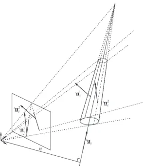
The legs of parallel robots usually have cylindrical cross-sections [25]. The edges of thei-th cylindrical leg are given,

in the camera frame, by [14] (Fig 1):

c_n1 i = − cos θichi− sin θicui×chi (3) c_n2 i = + cos θichi− sin θicui×chi (4) where cos θi = p_c h2 i − R2i . c_h i, sin θi = Ri/chi and (c_u

i,chi,chi) are the Binormalized Pl¨ucker coordinates of the

cylinder axis andRi is the cylinder radius.

It was also shown in [14] that the leg orientation, expressed in the camera frame, is given by

c_u i= c_n1 i ×cn2i kc_n1 i ×cn2ik (5) Let us remark that each cylinder edge is a line in space, with Binormalized Pl¨ucker expressed in the camera frame

(c_u i,cn j i,cn j i) (Fig 1).

2_{In the following of the paper, the superscript before the vector denotes}

the frame in which the vector is expressed (“b” for the base frame, “c” for the camera frame and “p” for the pixel frame). If there is no superscript, the vector can be written in any frame.

c_n i c_u i 1 c_n i 2 c_n i 1 c_n i 2 n

Fig. 1. Projection of a cylinder in the image

C. Leg direction based visual servoing

The proposed control approach was to servo the leg direc-tions cu_i [12]. Some brief recalls on this type of controller are done below.

1) Interaction matrix: Visual servoing is based on the so-called interaction matrix LT [26] which relates the instanta-neous relative motion Tc = cτ_c −cτ_s between the camera

and the scene, to the time derivative of the vectors of all the

visual primitives that are used through:

˙s = LT(s)Tc (6)

wherecτ_candcτ_sare respectively the kinematic screw of the

camera and the scene, both expressed in Rc, i.e. the camera

frame.

In the case where we want to directly control the leg directions c_u

i, and if the camera is fixed, (6) becomes: c_˙u

i= MTi cτc (7)

where MT

i is the interaction matrix for the leg i.

2) Control: For the visual servoing of a robot, one achieves exponential decay of an error e(s, sd) between the current

primitive vectors and the desired one sd using a proportional

linearizing and decoupling control scheme of the form (if the scene is fixed):

c_τ

c= λˆLT+(s)e(s, sd) (8)

where cτ_c is used as a pseudo-control variable and the

superscript “+” corresponds to the matrix pseudo-inverse. The visual primitives being unit vectors, it is theoretically more elegant to use the geodesic error rather than the stan-dard vector difference. Consequently, the error grounding the proposed control law will be:

ei =cui×cudi (9)

where cu_di is the desired value ofcu_i.

It can be proven that, for spatial parallel robots, matrices

Mi are in general of rank 2 [12] (for planar parallel robots,

they are of rank 1). As a result, for spatial robots with more than 2 degrees of freedom (dof ), the observation of several independent legs is necessary to control the end-effector pose. An interaction matrix MT can then obtained by stacking k

matrices MT_i ofk legs.

Finally, a control is chosen such that e, the vector stacking the errors ei ofk legs, decreases exponentially, i.e. such that

˙e = −λe (10)

It should be mentioned that, in reality, it is not possible to ensure a perfect exponential decrease of e if the dimension of

e is larger than the number of degrees of freedom [27], [28].

Then, introducing LT_i = − [c_u di]×M

T

i, where [cudi]× is

the cross product matrix associated with the vector cu_di, the combination of (9), (7) and (10) gives

c_τ

c= −λLT+e (11)

where LT can be obtained by stacking the matrices LT_i of k

legs. The conditions for the rank deficiency of matrix LT, as well as the conditions that lead to local minima [18] of the Eq. (11) are discussed in Section III.

This expression can be transformed into the control joint velocities:

˙q = −λc_Jinv_LT+_{e (12)}

wherec_Jinv_{is the inverse Jacobian matrix of the robot relating}

the end-effector twist to the actuator velocities, i.e.c_Jinv c_τ c=

˙q.

D. Statement of the problem

It is obvious that the objective of any controller is to ensure two main properties: the observability of some given robot elements (in our case, the end-effector) and the controllability of the robot. For that, any controller is based on the obser-vation of some features (the encoder positions, velocity and acceleration in usual controllers, or some robot parts in sensor-based controllers) which must ensure that:

1) it is possible to properly estimate the pose (and also eventually the velocity and acceleration) of the end-effector (which is an external property of the robot), 2) it is also possible to estimate the internal state of the

robot (position, velocity and acceleration of any body) as this information is necessary for achieving the control (for instance, in the controller defined at Eq. (12), the computation of the inverse kinematic Jacobian matrix

c_Jinv _{is necessary, and its expression is usually a}

function of the active (and sometimes also passive) joint variables).

Ideally, from the observation of a minimal set of given features (denoted as a minimal basis), the mapping involved for the estimation of the end-effector pose must be a global diffeomorphism (Fig. 2(a)). However, in the case of parallel robots in classical encoder-based controllers, a given set of encoder positions usually leads to the computation of several possible end-effector poses [25] which are called the robot

Minimal basis

of observed

features (s)

End-effector

pose

Robot internal

state (all joint configurations)

observability

controllability

(a) when a global diffeomorphism exists

Minimal basis

of observed

features (s)

Assembly

mode 1

observability

controllability

Assembly

mode n

End-effector pose

Possible leg

configuration 1

Possible leg

configuration n

Robot internal state

(b) when there is no global diffeomorphism

Fig. 2. Ensuring the observability and controllability of the robot through a proper feature observation.

assembly modes. These assembly modes correspond to some given aspects of the workspace (i.e. workspace zones which are seperated by singularities), which means that the robot cannot freely move in all the workspace areas. Thus, there is no global diffeomorphism between the encoder positions and the end-effector pose (Fig. 2(b)). To overcome this diffi-culty, usually, the parallel robot is moved in only one given workspace aspect for which the assembly mode can be strictly known.

By extension, if we cannot strictly know the end-effector pose, we cannot also correctly estimate the internal robot state (position, velocity and acceleration of any body)3_{. The} question is thus: what should be the minimal basis of the observed features that is able to ensure that we are able to stricly estimate both the end-effector pose and the robot

3_{It is necessary to mention that, for a given end-effector pose, several}

leg configurations (called working modes) may exist. However, for the large majority of parallel robots for which each leg is made of at most two moving elements, if we strictly know the end-effector pose plus the pose of an element of a considered leg, the leg configuration can be uniquely defined.

internal state, i.e. to strictly ensure the robot controllability? In the next Sections, it is shown that the use of a tool named the “hidden robot model” can help analyze the controllability of parallel robots when the canonical basis of the observed features is partially made of the robot leg directions. We first introduce the concept of the hidden robot model and then show how it can be used for the analysis of the controllability.

III. THE CONCEPT OF HIDDEN ROBOT MODEL The concept of the hidden robot model was first introduced in [19] for the visual servoing of the GS platform. In this paper, it has been demonstrated that the leg-direction-based visual servoing (Section II) of such robots intrinsically involves the appearance of a hidden robot model, which has assembly modes and singularities different from the real robot. It was shown that the concept of the hidden robot model fully explains the possible non-convergence of the observed robot to the desired final pose and that it considerably simplifies the singularity analysis of the mapping involved in the controller. The concept of the hidden robot model comes from the following observation: in the classical control approach, the encoders measure the motion of the actuator; in the previously described control approach (Section II), the leg directions or leg edges are observed. So, in a reciprocal manner, one could wonder to what kind of virtual actuators such observations correspond. The main objective of this Section is to give a general answer to this question.

A. How to define the legs of the hidden robots

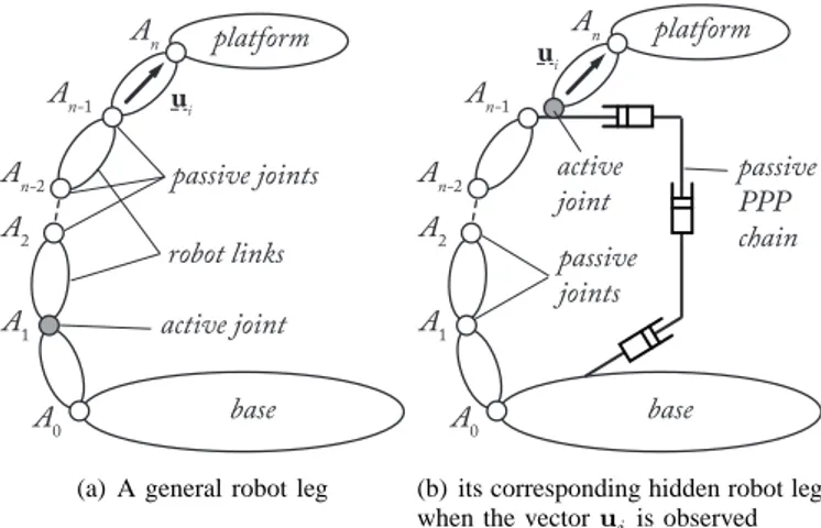
Let us consider a general leg for a parallel robot in which the direction u_iof a segment is observed (Fig. 3(a) – in this figure, the last segment is considered observed, but the following explanations can be generalized to any segment located in the leg chain). In what follows, we only consider that we observe the leg direction u_i, and not the leg edges in the image space, as the leg edges are only used as a measure of u_i. So the problem is the same, except in the fact that we must consider the singularity of the mapping between the edges and u_i, but this problem is well handled: these singularities appear when

n1_i and n2_i are collinear, i.e. the cylinders are at infinity [14]. In the general case, the unit vector u_i can obviously be parameterized by two independent coordinates, that can be two angles, for example the anglesα and β of Fig. 4 defined

such that cos α = x · v = y · w (where v and w are defined

such that z· v = z · w = 0) and cos β = u · x. Thus α is

the angle of the first rotation of the link direction u_i around

z and β is the angle of the second rotation around v.

It is well known that a U joint is able to orient a link around two orthogonal axes of rotation, such as z and v. Thus U joints can be the virtual actuators we are looking for, with generalized coordinates α and β. Of course, other solutions

can exist, but U joints are the simplest ones.

If a U joint is the virtual actuator that makes the vector u_i move, it is obvious that:

• if the value of u

i is fixed, the U joint coordinatesα and

ui platform base A0 A₁ A2 A_n A_n-1 An-2 passive joints active joint robot links

(a) A general robot leg

u_i platform base A0 A₁ A2 An A_n-1 An-2 passive joints active joint passive PPP chain

(b) its corresponding hidden robot leg when the vector uiis observed

Fig. 3. A general robot leg and its corresponding hidden robot leg when the vector u_iis observed

x

y

z

_u

: observed

direction

w

α

β

v

virtual

cardan

joint

v

.

z

=0

w

.

z

=0

Fig. 4. Parameterization of a unit vector uiwith respect to a given frame x,

yand z

• if the value of u

i is changing, the U joint coordinatesα

andβ must also vary.

As a result, to ensure the aforementioned properties for α

and β if ui is expressed in the base or camera frame (but

the problem is identical as the camera is considered fixed on the ground), vectors x, y and z of Fig. 4 must be the vectors defining the base or camera frame. Thus, in terms of properties for the virtual actuator, this implies that the first U joint axis must be constant w.r.t. the base frame, i.e. the U joint must be attached to a link performing a translation w.r.t. the base frame4_.

However, in most cases, the real leg architecture is not composed of U joints attached to links performing a translation w.r.t. the base frame. Thus, the architecture of the hidden robot leg must be modified w.r.t. the real leg such as depicted in Fig. 3(b). The U joint must be mounted on a passive kinematic chain composed of at most 3 orthogonal passive P joints that ensures that the link to which it is attached performs a translation w.r.t. the base frame. This passive chain is also linked to the segments before the observed links so that they do not change their kinematic properties in terms of motion. Note that:

4_{In the case where the camera is not mounted on the frame but on a moving}

link, the virtual U joint must be attached on a link performing a translation w.r.t. the considered moving link.

• it is necessary to fix the PPP chain on the preceding leg

links because the information given by the vectors u_i is not enough to rebuild the full platform position and ori-entation: it is also necessary to get information (obtained via simplified kinematic models [14]) on the location of the anchor point An−1 of the observed segment. This

information is kept through the use of the PPP chain fixed on the first segments;

• 3 P joints are only necessary if and only if the pointA_n−1

describes a motion in the 3D space; if not, the number of P joints can be decreased: for example, in the case of the GS platform presented in [19], the U joint of the leg to control was located on the base, i.e. there was no need to add passive P joints to keep the orientation of its first axis constant;

• when the vector u

iis constrained to move in a plane such

as for planar legs, the virtual actuator becomes an R joint which must be mounted on the passive PPP chain (for the same reasons as mentioned previously).

For example, let us have a look at the RU leg with one actuated R joint followed by a U joint of Fig. 5(a). Using the previous approach, its virtual equivalent leg should be an{R–

PP}–U leg (Fig. 5(b)), i.e. the U joint able to orient the vector u_iis mounted on the top of a R–PP chain that can guarantee that:

1) the link on which the U joint is attached performs a translation w.r.t. the base frame,

2) the pointC (i.e. the centre of the U joint) evolves on a

circle of radiuslAB, like the real leg.

It should be noted that, in several cases for robots with a lower mobility (i.e. spatial robots with a number of dof less than 6, or planar robots with a number of dof less than 3), the last joint that links the leg to the platform should be changed so that, if the number of observed legs is inferior to the number of real legs, the hidden robot keeps the same number of controlled dof (see [21], [22]).

It should also be mentioned that we presented above the most general methodology that is possible to propose, but it is not the most elegant way to proceed. In many cases, a hidden robot leg architecture can be obtained such that less modifications w.r.t the real leg are achieved. For example, the R–PP chain of the hidden robot leg {R–PP}–U (Fig. 5(b))

could be equivalently replaced by a planar parallelogram (Π)

joint without changing the aforementioned properties of the U virtual actuator (Fig. 5(c)), i.e. only one additional joint is added to obtain the hidden robot leg (note that we consider that aΠ joint, even if composed of several pairs, can be seen

as one single joint, as in [20]).

In what follows in this paper, this strategy for finding the simplest hidden robot legs (in terms of architectural simplicity) is adopted for the studied robots.

B. How to use the hidden robot models for understanding the surprising and unanswered results arising from the use of leg-direction-based controllers

The aim of this Section is to show how to use the hidden robots to answer points 1 to 4 enumerated in the introduction

u A B C U joint R joint (a) A RU leg u PP chain A B C U joint mounted on the PP chain R joint

(b) Virtual{R–PP}–U leg

Planar parallelogram (Π) joint u A B C U joint mounted on the link BD R joint _E D

(c) Virtual ΠU leg

Fig. 5. A RU leg and two equivalent solutions for its hidden leg

of the paper.

Point 1: the hidden robot model can be used to explain why the observed robot which is composed ofn legs can be controlled

using the observation of only m leg directions (m < n).

To answer this point, let us consider a general parallel robot composed of 6 legs (one actuator per leg) and having six dof. Using the approach proposed in Section III-A, each

u

u

assembly modes

u

u

Fig. 6. Two configurations of a five bar mechanism for which the directions

uiare identical (for i = 1, 2)

observed leg will lead to a modified virtual leg with at least one actuated U joint that has two degrees of actuation. For controlling 6 dof, only 6 degrees of actuation are necessary, i.e. three actuated U are enough (as long as the motions of the U joints are not correlated, i.e. the robot is fully actuated). Thus, in a general case, only three legs have to be observed to fully control the platform dof.

Point 2: the hidden robot model can be used to prove that there does not always exist a global diffeomorphism between the Cartesian space and the leg direction space.

Here, the answer comes directly from the fact that the real controlled robot may have a hidden robot model with different geometric and kinematics properties. This means that the hidden robot may have assembly modes and singular configurations different from those of the real robot. If the initial and final robot configurations are not included in the same aspect (i.e. a workspace area that is singularity-free and bounded by singularities [25]), the robot will not be able to converge to the desired pose, but to a pose that corresponds to another assembly mode that has the same leg directions as the desired final pose (see Fig. 6).

Point 3: the hidden robot model simplifies the singularity analysis of the mapping between the leg direction space and the Cartesian space by reducing the problem to the singularity analysis of a new robot.

The interaction matrix MT involved in the controller gives the value of c˙u as a function of c_τ

c. Thus, MT is the

inverse kinematic Jacobian matrix of the hidden robot (and, consequently, MT+ is the hidden robot kinematic Jacobian matrix). Except in the case of decoupled robots [29]–[31], the kinematic Jacobian matrices of parallel robots are not free of singularities.

different kinds of singularity can be observed [32]5_:

• the Type 1 singularities that appear when the robot

kinematic Jacobian matrix is rank-deficient; in such con-figurations, any motion of the actuator that belongs to the kernel of the kinematic Jacobian matrix is not able to produce a motion of the platform,

• the Type 2 singularities that occur when the robot inverse

kinematic Jacobian matrix is rank-deficient; in such con-figurations, any motion of the platform that belongs to the kernel of the inverse kinematic Jacobian matrix is not able to produce a motion of the actuator. And, reciprocally, near these configurations, small motions of the actuators lead to large platform displacements, i.e. the accuracy of the robot becomes very poor,

• the Type 3 singularities that appear when both the robot

kinematic Jacobian and inverse kinematic Jacobian ma-trices are rank-deficient.

Thus,

• finding the condition for the rank-deficiency of MT is

equivalent to finding the Type 2 singularities of the hidden robot,

• finding the condition for the rank-deficiency of MT+ is

equivalent to finding the Type 1 singularities of the hidden robot.

Since a couple of decades ago, many tools have been developed by the mechanical design community for finding the singular configurations of robots. The interested reader could refer to [25], [34]–[36] and many other works on the Grassmann Geometry and Grassmann-Cayley Algebra for studying the singular configurations problem. In what follows in the paper, these tools are used but only the final results concerning the singular configuration conditions are given. Point 4: the hidden robot model can be used to certify that the robot will not converge to local minima.

The robot could converge to local minima if the matrix

MT+ is rank deficient, i.e. the hidden robot model encounters a Type 1 singularity. As mentioned above, many tools have been developed by the mechanical design community for finding the singular configurations of robots and solutions can be provided to ensure that the hidden robot model does not meet any Type 1 singularity.

The next Section explains how to use the hidden robot concept to check the controllability of robots and, eventually for robots which are not controllable, how to modify the controller to ensure their controllability.

IV. CONTROLLABILITY ANALYSIS

Thanks to the hidden robot concept, it is possible to ana-lyze the controllability of parallel robots and to define three categories of robots:

5_{There exist other types of singularities, such as the constraint}

singular-ities [33], but they are due to passive constraint degeneracy only, and are not involved in the mapping between the leg directions space and the robot controlled Cartesian coordinate space.

1) robots which are not controllable using the leg direction observation: this case will appear if, for a given set of observed features s, the mapping involved in the

controller for estimating the end-effector pose is singular for an infinity of robot configurations (in other words, the end-effector configuration is not observable), 2) robots which are partially controllable in their whole

workspace using the leg direction observation: this case will appear if, for a given set of observed features s,

the mapping involved in the controller is not a global diffeomorphism (i.e. a given set of observed features s

may lead to several possible end-effector configurations – Fig. 2(b)),

3) robots which are fully controllable in their whole workspace using the leg direction observation: this case will appear if, for a given set of observed features

s, the mapping involved in the controller is a global

diffeomorphism (i.e. a given set of observed features s

leads to a unique end-effector configuration – Fig. 2(a)). Families of robots belonging to these categories are defined thereafter. Moreover, after this classification, insights are pro-vided to ensure that all robots could be controllable by adding supplementary observations.

A. Robots which are not controllable using the leg direction observation

With the hidden robot concept, it is possible to find classes of robots which are not controllable using leg observations, and this without any mathematical derivations. These robots are those with a hidden robot model which is architecturally singular (whatever the number of observed legs). In other words, the hidden robots have unconstrained dof.

Three main classes of parallel robots belong to this category (the list is not exhaustive, but groups the most usual and known robots in the community):

• robots with legs whose directions are constant for all

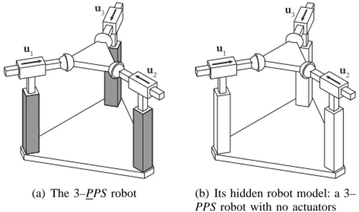
robot configurations: for these robots, the anchor point location of the observed links cannot be found through the use of the simplified kinematic models. This are the cases of planar 3–PPR (Fig. 7) and 3–PPR robots [25], [37] and of certain spatial robots such as the 3–[PP]PS robots6 _{(with 3–PPS robots (with 3 dof [38] (Fig. 8)} or with 6 dof – e.g. the MePaM [36])). It is obvious that for robots with legs whose directions are constant in the whole workspace, it is not possible to estimate the platform pose from the leg directions only.

• robots with legs whose directions are constant for an

infinity of (but not all) robot configurations: this is the case of PRRRP robots with all P parallel (Fig. 9(a)) and of Delta-like robots actuated via P joints for which all P are parallel (such as the UraneSX (Fig. 10) or the I4L [39], [40]). It was shown in [16] through the analysis of the rank deficiency of the interaction matrix that it was not possible to control such types of robots using leg direction observation. Considering this problem with

6_{[PP] means an active planar chain able to achieve two dof of translation,}

u₁

u₂ u₃

(a) The 3–P P R robot

u₁

u₂ u₃

(b) Its hidden robot model: a 3–

P P R robot with no actuators

Fig. 7. The 3–P P R robot and its hidden robot model (the grey joints denote the actuated joints)

u₁

u₂ u₃

(a) The 3–PPS robot

u₁

u₂ u₃

(b) Its hidden robot model: a 3– PPS robot with no actuators Fig. 8. The 3–PPS robot and its hidden robot model (the grey joints denote the actuated joints)

u₁ u₂

(a) The PRRRP robot

unconstrained translation

u₁ u₂

(b) Its hidden robot model: a PRRRP robot

Fig. 9. The PRRRP robot and its hidden robot model (the grey circles denote the actuated joints)

the hidden robot concept is very easy. For example, in the case of the PRRRP robot with parallel P joints, the hidden robot has a PRRRP architecture (Fig. 9(b)), where the parallel P joints are passive. This robot is well-known to be architecturally singular as there is no way to control the translation along the axis of the parallel P joints. This result can be easily extended to the cases of the hidden robots of the UraneSX and the I4L (Fig. 10).

• robots with legs whose directions vary with the robot

configurations but for which all hidden robot legs contain active R joints but only passive P joints: the most known robot of this category will be the planar 3–PRP robot for which the hidden robot model is a 3–PRP which is known to be uncontrollable [25], [37] (Fig. 11).

u₁ u3

u₂

(a) Schematics of the architecture: a 3– PUU robot with the three actuated P joints in parallel platform P active U joint passive U joint passive P joint passive motion of the platform u_i

(b) Its hidden robot leg: a PUU leg; thus, the hidden robot is a 3–PUU robot with the three pas-sive P joints in parallel leading to an uncontrollable translation along the P joints direction

Fig. 10. The UraneSX robot and its hidden robot leg

u₁

u2

u₃

(a) The 3–P RP robot

u₁

u₂

u₃

(b) Its hidden robot model: a 3–

P RP robot known to be

uncon-trollable

Fig. 11. The 3–P RP robot and its hidden robot model (the grey joints denote the actuated joints)

B. Robots which are partially controllable in their whole workspace using the leg direction observation

The hidden robot model can be used to analyze and under-stand the singularities of the mapping and to study if a global diffeomorphism exists between the space of the observed element and the Cartesian space. However, not finding a global diffeomorphism does not necessarily mean that the robot is not controllable. This only means that the robot will not be able to access certain zones of its workspace (the zones corresponding to the assembly modes of the hidden robot model which are not contained in the same aspect as the one of the robot initial configuration). This is of course a problem if the operational workspace of the real robot is fully or partially included in these zones.

Robots belonging to this category are probably the most numerous. They are those for which the hidden robot models have several possible assembly modes, whatever is the number of observed leg directions. Presenting an exhaustive list of robots of this category is totally impossible because it requires the analysis of the assembly modes of all hidden robot models for each robot architecture. However, some examples can be provided.

(a) The Gough-Stewart platform from DeltaLab: a 6–U P S robot

A 1 B1 C u 1 A2 B2 u2 A 3 B3 u3 P1 P2 P3 P4

(b) Its hidden robot model: a 3–

U P S robot (when three legs are

observed)

Fig. 12. The Gough-Stewart platform and its hidden robot model

u1

u3 u2

u4

(a) The Adept Quattro: a 4–R− 2− U S robot Fixed base Articulated moving platform Pi Pj ui uj

(b) Its hidden robot model: a 2–

Π− 2 − U U robot (when two

legs are observed)

Fig. 13. The Adept Quattro and its hidden robot model

Examples of such types of robots (the Gough-Stewart platform (Fig. 12) and the Adept Quattro (Fig. 13)) have been presented in [19], [21], [22]. More specifically, in [21], [22], it was shown (numerically but also experimentally) that the Adept Quattro [41] controlled through leg direction observation has always at least two assembly modes of the hidden robot model, whatever the number of observed legs. As a result, some areas of the robot workspace were never reachable from the initial configuration. Figure 14 shows a desired robot configuration that was impossible to reach even if all robot legs were observed.

It should be mentioned that, even if it is out of the scope of the present paper, it can be verified if the operational workspace of the real robot is fully or partially included in the aspects of the hidden robot models. This problem may be complex, but can be solved using some advanced tools such as interval analysis [25] or Cylindrical Algebraic Decomposition (CAD) [42]. It should also be mentioned that a Maple library for the CAD has been developed by IRCCyN and is available under request on [43].

C. Robots which are fully controllable in their whole workspace using the leg direction observation

Robots of this category are those for which there exists a global diffeomorphism between the leg direction space and Cartesian space for all workspace configurations. Their hidden robot models have only one possible assembly mode. Once again, presenting an exhaustive list of robots of this category is totally impossible because it requires the analysis of the assembly modes of all hidden robot models for each robot architecture. −0.8 −0.6 −0.4 −0.2 0 0.2 0.4 0.6 −1 0 1 −0.8 −0.6 −0.4 −0.2 0 0. 2 x (m) y (m) z (m) final pose desired pose starting pose trajectory

Fig. 14. Desired and final position of the Quattro when all legs are observed.

Fixed base

Moving platform

u₁

u₂ u₃

(a) Kinematic chain

platform P active U joint passive U joint passive P joint passive motion of the platform ui

(b) The hidden robot leg

Fig. 15. The Orthoglide and its hidden robot leg.

However, we show here for the first time robots belonging to this category. Let us consider the Orthoglide [44] designed at IRCCyN (Fig. 15(a)). This robot is a mechanism with 3 translational dof of the platform. It is composed of three identical legs made of PRΠR architecture, or also with PUU

architecture, the P joint of each leg being orthogonal. Let us consider the second type of leg which is simpler to analyze (even if the following results are also true for the first type of leg). If the link between the two passive U joints is observed, from Section III, the hidden robot leg has a PUU architecture with, of course, two degrees of actuation. As a result, for controlling the three dof of the platform, only two legs need to be observed.

For a fixed configuration of the actuated U joint, each leg tip has the possibility to freely move on a line directed along the corresponding P joint direction: this line corresponds to the free motion of the platform due to the virtual passive P joint of each leg, when other legs are disconnected (Fig. 15(b)). Then, estimating the robot pose is equivalent to finding the intersection of two lines in space (three lines if the three legs are observed). As a result, in a general manner, the forward kinematic problem (fkp) may have:

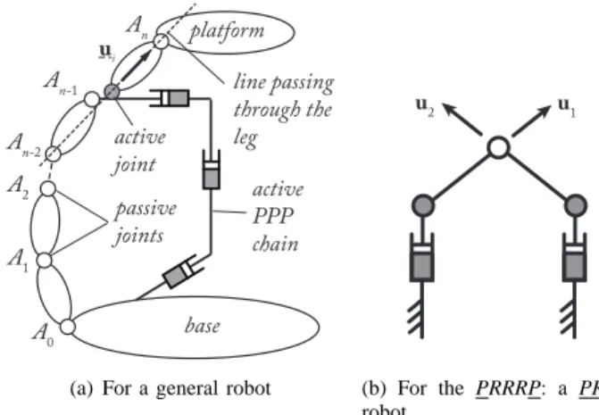
u_i platform base A₀ A₁ A₂ A_n A_n-1 A_n-2 passive joints active joint active PPP chain line passing through the leg

(a) For a general robot

u₁ u₂

(b) For the PRRRP: a PRRRP robot

Fig. 16. The hidden robot leg when the Pl¨ucker coordinates of the line passing through the axis of the leg are observed.

• zero solutions (impossible in reality due to the robot

geometric constraints),

• an infinity of solutions if and only if the P joints are

parallel (not possible for the Orthoglide as all P joints are orthogonal),

• one solution (the only possibility).

Moreover, a simple singularity analysis of all the possible hidden robot models of the Orthoglide could show that they have no Type 2 singularities (which is coherent with the fact that the fkp has only one solution).

By extension of these results, it could be straightforwardly proven that all robots with 3 translational dof of the platform, or with Sch¨onflies motions (3 translational dof of the platform plus one rotational dof about one fixed axis), which are composed of identical legs made of PRΠR architecture, or

also with PUU architecture and for at least two P joints are not parallel (e.g. the Y-STAR [45]) are fully controllable in their whole workspace using the leg direction observation.

D. Robots which become fully controllable in their whole workspace if additional information is used

After this classification, one additional question is to know if, by adding additional information in the controller, the robots which were uncontrollable or partially controllable in their whole workspace can become fully controllable.

For example, it was very recently proven in [46] that, from the projection of the cylindrical leg in the image plane (Fig. 1), it is not only possible to estimate the leg direction, but also the Pl¨ucker coordinates of the line passing through the axis of the cylinder, i.e. the direction and location in space of this line. Using this information leads to a modification of the virtual leg as shown in Fig. 16(a): the additional prismatic chain, instead of being passive, becomes active.

This additional information can solve many issues of con-trollability mentioned above. For example, by estimating the Pl¨ucker coordinates of the line passing through its legs, the PRRRP robot of Section IV-A becomes controllable as the hidden robot model becomes a PRRRP robot (Fig. 16(b)) which is fully controllable.

However, this information may not be enough for some categories of robots, such as for the MePaM [36] for which it was shown in [47] that using the Pl¨ucker coordinates of the line passing through the legs leads to a robot which is partially controllable in its whole workspace (eight different assembly modes of the hidden robot model may appear). A similar result could be proven for the GS platform for which the Pl¨ucker coordinates do not bring any additional useful information in the controller. For such robots, two main solutions are possible:

• if the robot operational workspace is included in one

given aspect of the hidden robot model, the controller may be sufficient to fully control the robot in its opera-tional workspace,

• other features (such as other robot elements (joint

loca-tions, other links, etc.)) should be observed to complete the missing information.

Regarding this last point, it is necessary to mention that, in this paper, we only focus on the information that we could extract from the camera, and not from other sensors. Indeed, combining information from different sensors implies some issues of multi-sensor calibration which are not addressed here but that will be part of our future work.

V. ILLUSTRATIVE EXAMPLES A. Case study 1: a 3–PRR planar robot

1) Presentation of the robot under study: In the present section, we illustrate the present work by analyzing the controllability of a special type of planar 3–PRR robot with parallel P and two coincident platform joints (Fig. 17(a)). In the following of the paper, we consider that:

• q₁, q₂ and q₃ are the coordinates of the actuators of the

real robot,

• the lengths of segmentsA₁P , A₂P and A₃P are denoted

lA1P,lA2P andlA3B, respectively, and are equal, i.e.l =

lA1P = lA2P = lA3B,

• the controlled point on the effector is the point P with

coordinatesx and y along the x and y axes, respectively,

• the orientation of the platform with respect to the x axis

is parametrized by the angle φ,

• the distance between the joints located at points P and

B is denoted as d.

For this mechanism, Type 1 singularities appear when u_i is orthogonal to the direction of the prismatic guide of the leg

i (Fig. 17(b)). These singularities represent some workspace

boundaries.

For this mechanism, Type 2 singularities appear:

• when u

1and u2are collinear (Fig. 18(a)): they appear if

and only if the legs 1 and 2 are in antagonistic working modes (‘+−’ or ‘−+’, see Fig. 17(b)) for x = a1/2

for any y and φ, i.e. they never appear when the legs 1

and 2 are in working modes ‘++’ or ‘−−’ such as in

Fig. 17(a).

• or when u₂ and

−−→

P B are collinear (Fig. 18(b)): they

may appear for any x and y if and only if the robot

reaches constant platform orientations defined bycos φ = a2/(d + l) or cos φ = a2/ |d − l|.

A

A

A

P

(x,y)

B

φ

x

y

O

q

q

q

u

u

u

a

a

(a) Kinematic architecture of the robot

A

O

Fig. 17. Schematics of the 3–PRR robot.

A

A

A

B

x

y

(a) Example of the first case of Type 2 singularity

A

_A

A

B

x

y

P

(b) Example of the second case of Type 2 singularity

Fig. 18. Singularities of the 3–PRR robot.

2) Analysis of the possible hidden robot models: Case 1: Let us now assume that we want to control the 3–PRR robot depicted at Fig. 17(a) by using the observation of its leg directions u_i(see Section II). From Section III, we know that using such a control approach involves the appearance of a hidden robot model. This hidden robot model can be found by straightforwardly using the results of Section III and is a 3–PRR robot shown in Fig. 19(a). This robot is known to be architecturally singular (it can freely move along the y axis) and can not be controlled by using only the observation of its leg directions u_i.

Case 2: As a result, one would logically wonder what should

be the necessary information to retain in the controller to servo the robot. By using the results of Section IV-D, we know that, from the projection of the cylindrical leg in the image plane, it is not only possible to estimate the leg direction, but also the Pl¨ucker coordinates of the line passing through the axis of the cylinder, i.e. the direction and location in space of this line. Let us consider that we add this information for the estimation of the leg 1 position only. Modifying the hidden robot model according to Fig. 16(a), the corresponding robot model hidden in the controller is depicted in Fig. 19(b): this is a PRR–{2–PRR} robot which is not architecturally singular.

In other words, using the Pl¨ucker coordinates of the line for leg 1 involves to actuate both the first P and R joints of the corresponding leg, i.e. the virtual leg is a PRR leg. For the PRR–{2–PRR} robot, it is possible to prove that two assembly

modes exist which are separated by a Type 2 singularity at

φ = 0 or π (for any x and y). For both assembly modes,

the end-effector position is the same, while the orientation is different. Thus, the robot is not fully controllable in its whole workspace.

Case 3: From the result that, using the Pl¨ucker coordinates of the line passing through the axis of the cylinder, the leg of the virtual robot becomes a PRR leg, it is possible to understand what is the minimal set of information to provide to the controller to fully control the robot in the whole workspace: we need to use the Pl¨ucker coordinates of the lines passing through legs 1 and 3 and the direction of the leg 2. In such a case, the hidden robot model is a PRR–{2–PRR} robot

depicted in Fig. 19(c). It is possible to prove that this robot has no Type 2 singularity and can freely access its whole workspace.

3) Simulation results: Simulations are performed on an Adams mockup of the 3–PRR robot with the following values for the geometric parameters:l = 1 m, d = 0.4 m, a1= 0.4 m

anda2 = 0.25 m. This virtual mockup is connected to

Mat-lab/Simulink via the module Adams/Controls. The controller presented in Section II is applied with a value of λ assigned

to 20.

The initial configuration of the robot end-effector isx0 =

0.20 m, y0 = 0.98 m and φ0 = −45 deg. We want to reach

the end-effector configurationxf = 0.20 m, yf = 1.03 m and

φf = −10 deg. For that, we use the three possible controllers

(Cases 1, 2 and 3) proposed in the previous Section and simulate the robot behavior with the Adams mockup during 1 second. For the three cases, the errors on the used observed features (either the leg directions or the Pl¨ucker coordinates of the lines) tends to zero at the end of the simulation. However, this is not necessary the case for the end-effector configuration (Table I).

With the controller of Case 1 based on the observation of the leg directions only, the robot is not able to attain the final end-effector configuration. Moreover, the end-effector position is unchanged (while its orientation has been modified) which is coherent with the results of the previous section: the corresponding hidden robot is architecturally singular and its motion along the y axis is uncontrollable.

For the two other controllers, the convergence towards the desired end-effector pose is achieved.

A

_A

A

P

B

x

y

O

(a) When all leg directions uiare observed (Case 1): a 3–PRR robot

A

_A

A

B

x

y

O

P

(b) When all leg directions uiand the Pl¨ucker coordinates of the line passing through the leg 1 are observed (Case 2): a PRR–{2–PRR} robot

A

A

A

B

x

y

O

P

(c) When all leg directions uiand the Pl¨ucker coordinates of the lines passing through the legs 1 and 3 are observed (Case 3): a PRR–{2–PRR} robot

Fig. 19. Hidden robots involved in the tested visual servoings of the 3–PRR robot.

Now, we change the desired end-effector configurationxf=

0.20 m, yf = 1.03 m and φf = +10 deg. The results for the

end-effector convergence are provided in Table II.

With the controller of Case 1, the results are unchanged: the robot is not able to reach the desired configuration.

With the controller of Case 2 based on the observation of the Pl¨ucker coordinates of the line passing through the leg 1 and the other leg directions, the robot attains the final end-effector position, but not the correct orientation. This is coherent with the results of the previous section: the corresponding hidden robot has two assembly modes with similar end-effector positions but different orientations. It can

TABLE I

FINAL END-EFFECTOR CONFIGURATION FOR THE DESIRED END-EFFECTOR CONFIGURATIONxf = 0.20M, yf= 1.03M ANDφf =−10DEG

x (m) y (m) φ (deg)

Case 1 0.20 0.98 −10

Case 2 0.20 1.03 −10

Case 3 0.20 1.03 −10

TABLE II

FINAL END-EFFECTOR CONFIGURATION FOR THE DESIRED END-EFFECTOR CONFIGURATIONxf = 0.20M, yf= 1.03M ANDφf = +10DEG

x (m) y (m) φ (deg)

Case 1 0.20 0.98 −10

Case 2 0.20 1.03 −10

Case 3 0.20 1.03 +10

be proven that, for the given robot geometric parameters, the two assembly modes of the PRR–{2–PRR} robot for the given

observed features at the desired final robot configuration are:

• x₁= 0.20 m, y₁= 1.03 m and φ₁= +10 deg, and • x₂= 0.20 m, y₂= 1.03 m and φ₂= −10 deg.

Thus, the robot has converged towards the second assembly mode, which was not the desired one. However, this second as-sembly mode was reached during the first simulation, because it is enclosed in the same workspace aspect corresponding to the initial robot configuration.

Finally, with the controller of Case 3 based on the obser-vation of the Pl¨ucker coordinates of the lines passing through the legs 1 and 3 and the leg 2 direction, the robot reached the desired configuration. This result was expected from the previous Section.

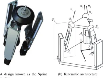
B. Case study 2: a 3–PRS spatial robot

1) Presentation of the robot under study: In the section, we analyze the controllability of a special type of spatial 3–PRS robot with parallel P joints which is indeed the kinematic rep-resentation of the Sprint Z3 machine from Siemens (Fig. 20). This robot is a zero-torsion robot [38], which means that it has three coupled dof which are usually taken as the translation along z and two rotations. Moreover, by taking into account the Tilt-and-Torsion angle formalism [48], it was demonstrated in [38] that the torsion angle was always zero. As a result, we propose to parameterize here the robot dof as:

• the translation along z of the pointB₁ denoted asz, • the first two angles of the Tilt-and-Torsion

parameteriza-tion [48], i.e. the azimuth and tilt angles denoted as φ

andθ respectively.

In the following of the paper, we consider that:

• q₁, q₂ and q₃ are the coordinates of the actuators of the

real robot (positions of pointsAi along z),

• due to the PRS architecture of each leg, the points B_i

(centers of the spherical joints) are constrained to move in a vertical plane denoted asPiwhose normal vector is

(a) A design known as the Sprint Z3 machine A1 _A 2 A3 B1 B2 B3 x y z u₁ u₂ u3 P1 (b) Kinematic architecture

Fig. 20. The spatial 3–PRS robot with parallel P joints.

• the relative orientation between P₁ andP₂ (andP₂ and

P3) is 120 deg. (obviously around the vertical axis z), • the lengths of segments A₁B₁, A₂B₂ and A₃B₃ are

denoted lA1B1, lA2B2 and lA3B3, respectively, and are

equal, i.e.l = lA1B1 = lA2B2 = lA3B3,

• the prismatic joints are equidistant with a fixed distance

d between them,

• the points B₁, B₂ and B₃ of the platform forms an

equilateral triangle of circumcircle with radius R.

For this mechanism, Type 1 singularities appear when

u_i is orthogonal to the direction of the prismatic guide of the leg i [38]. These singularities represent some workspace

boundaries. Type 2 singularities are more complex and are studied in [49].

2) Analysis of the possible hidden robot models: Case

1: Let us now assume that we want to control the 3–PRS robot depicted at Fig. 20 by using the observation of its leg directions u_i(see Section II). From Section III, we know that using such a control approach involves the appearance of a hidden robot model. This hidden robot model can be found by straightforwardly using the results of Section III and is a 3–PRS robot shown in Fig. 21(a). This robot is known to be architecturally singular (it can freely move along the z axis) and can not be controlled by using only the observation of its leg directions u_i.

Case 2: As a result, one would logically wonder what should be the necessary information to retain in the controller to servo the robot. For instance, let us use the Pl¨ucker coordinates of the line passing through the axis of the cylinder (see Section IV-D), i.e. the direction and location in space of this line. Let us consider that we add this information for the estimation of the legs 1 and 2 positions. Modifying the hidden robot model according to Fig. 16(a), the corresponding robot model hidden in the controller is depicted in Fig. 21(b): this is a{2–PRS}–PRS robot which is not architecturally singular. In

other words, using the Pl¨ucker coordinates of the line for legs 1 and 2 involves to actuate both the first P and R joints of the corresponding legs, i.e. the virtual legs are PRS legs. For the

{2–PRS}–PRS robot, it is possible to prove that two assembly

TABLE III

FINAL END-EFFECTOR CONFIGURATION FOR THE DESIRED END-EFFECTOR CONFIGURATIONzf = 0.40M, φf =−90DEG ANDθf= +10DEG

z (m) φ (deg) θ (deg)

Case 1 0.20 −90 −10

Case 2 0.40 −90 −10

Case 3 0.40 −90 +10

modes exist. Indeed, for this robot, when fixing the position of points B1 and B2 (which is the case when actuating the

P and R joints of the legs 1 and 2), the platform can freely rotate around(B1B2). Thus, B3performs a circle which will

intersect with the line corresponding of the free motion of the leg 3 tip when the platform is disconnected and the R joint is actuated only. As a result, the maximal number of solutions of the fkp is equal to two. For both assembly modes, the end-effector position is the same, while the orientation is different. Thus, the robot is not fully controllable in its whole workspace. Case 3: From the result that, using the Pl¨ucker coordinates of the line passing through the axis of the cylinder, the leg of the virtual robot becomes a PRS leg, it is possible to understand what is the minimal set of information to provide to the controller to fully control the robot in the whole workspace: we need to use all the Pl¨ucker coordinates of the lines passing through legs 1 to 3. In such a case, the hidden robot model is a 3–PRS robot depicted in Fig. 21(c). It is possible to prove that this robot has no Type 2 singularity and can freely access to its whole workspace.

3) Simulation results: Simulations are performed on an Adams mockup of the 3–PRS robot with the following values for the geometric parameters: l = 0.5 m, d = 0.4 m, R = 0.1 m. This virtual mockup is connected to Matlab/Simulink

via the module Adams/Controls. The controller presented in Section II is applied with a value ofλ assigned to 20.

The initial configuration of the robot end-effector is z0 =

0.20 m, φ0= −90 deg and θ0= −10 deg. We want to reach

the end-effector configuration zf = 0.40 m, φf = −90 deg

and θf = +10 deg. For that, we use the three possible

controllers (Cases 1, 2 and 3) proposed in the previous Section and simulate the robot behavior with the Adams mockup during 1 second. For the three cases, the errors on the used observed features (either the leg directions or the Pl¨ucker coordinates of the lines) tends to zero at the end of the simulation. However, this is not necessary the case for the end-effector configuration (Table III).

With the controller of Case 1 based on the observation of the leg directions only, the robot is not able to attain the final end-effector configuration. Moreover, the end-effector position is unchanged which is coherent with the results of the previous section: the corresponding hidden robot is architecturally singular and its motion along the z axis is uncontrollable.

With the controller of Case 2 based on the observation of the Pl¨ucker coordinates of the line passing through the legs 1 and 2 and the other leg direction, the robot attains the final end-effector position, but not the correct orientation.

A

A

B

y

z

O

B

A

B

x

(a) When all leg directions uiare observed (Case 1): a 3–PRS robot Assembly mode 1 Assembly mode 2

A

A

B

y

z

O

B

A

B

x

(b) When all leg directions u_iand the Pl¨ucker coordinates of the line passing through the legs 1 and 2 are observed (Case 2): a{2–PRS}–PRS robot

A

A

B

y

z

O

B

A

B

x

(c) When all leg directions u_iand the Pl¨ucker coordinates of the lines passing through the legs 1 and 3 are observed (Case 3): a 3–PRS robot

Fig. 21. Hidden robots involved in the tested visual servoings of the 3–PRS robot (projection in the yz plane – R and S joints at Aiand Bi, respectively, are drawn with the same symbol for the sake of clarity of the drawing).

This is coherent with the results of the previous section: the corresponding hidden robot has two assembly modes with similar end-effector positions but different orientations. It can be proven that, for the given robot geometric parameters, the two assembly modes of the{2–PRS}–PRS robot for the given

observed features at the desired final robot configuration are:

• z_f = 0.40 m, φ_f = −90 deg and θ_f = −10 deg, and • z_f = 0.40 m, φ_f = −90 deg and θ_f = +10 deg.

Thus, the robot has converged towards the second assembly

mode, which was not the desired one. However, this second as-sembly mode was reached during the first simulation, because it is enclosed in the same workspace aspect corresponding to the initial robot configuration.

Finally, with the controller of Case 3 based on the obser-vation of the Pl¨ucker coordinates of the lines passing through the legs 1 to 3, the robot reached the desired configuration. This result was expected from the previous Section.

C. Discussion

The results from the simulations show the real added value of the hidden robot concept. The hidden robot being a tangible visualization of the mapping between the observation space and the real robot Cartesian space, it is possible:

• to prove if the studied robot is controllable or not in its

whole workspace by the use of quite simple mechanism analysis tools,

• to understand the features to observe to ensure the

con-trollability of the robot in its whole workspace. To conclude this part, it is necessary to mention that:

• in our simulations, we have considered that the observed

features were not noisy, which is not true in reality. This has been simply assumed for two main reasons: (i) robustness of these types of controllers was already shown in previous works (e.g. [12], [14], [22]) and (ii) adding noise would have made the analysis of the convergence results in the controllers of Case 1 and 2 more difficult to explain, without bringing any added value to these simulations.

• the results for the controller of Case 3 for the first

case study would have been the same if the Pl¨ucker coordinates of the line 2 were observed instead of those of the line 1. The choice of the best leg to observe could have been done by a procedure presented in [19] which ensures to select the legs that lead to the best end-effector accuracy. However, this was out of the scope of the present paper.

• in the whole paper, it is considered that the sensor

measurement space is the same as the leg direction space. However, for example using a camera, the leg directions are not directly measured but rebuilt from the observation of the legs limbs projection in the 2D camera space [12]. Thus, for the leg reconstruction, the mapping between the camera space and the real 3D space is involved, and it is not free of singularities (see [50] for an example of mapping singularities). In the neighborhood of map-ping singularities, the robot accuracy will also tend to decrease. As a result, this mapping should be considered in the accuracy computation and in the selection of the legs to observe.

VI. CONCLUSIONS

This paper has presented a tool named the “hidden robot concept” that is well addressed for analyzing the controllability of parallel robots in leg-observation-based visual servoing techniques. It was shown that the mentioned visual servoing