The Stability and Stiffness Analysis of a Dual-Triangle Planar Rotation Mechanism

HAL Id: hal-03147414

https://hal.archives-ouvertes.fr/hal-03147414

Submitted on 19 Feb 2021

HAL is a multi-disciplinary open access

archive for the deposit and dissemination of

sci-entific research documents, whether they are

pub-lished or not. The documents may come from

teaching and research institutions in France or

abroad, or from public or private research centers.

L’archive ouverte pluridisciplinaire HAL, est

destinée au dépôt et à la diffusion de documents

scientifiques de niveau recherche, publiés ou non,

émanant des établissements d’enseignement et de

recherche français ou étrangers, des laboratoires

publics ou privés.

The Stability and Stiffness Analysis of a Dual-Triangle

Planar Rotation Mechanism

Wanda Zhao, Anatol Pashkevich, Alexandr Klimchik, Damien Chablat

To cite this version:

Wanda Zhao, Anatol Pashkevich, Alexandr Klimchik, Damien Chablat. The Stability and Stiffness

Analysis of a Dual-Triangle Planar Rotation Mechanism. ASME 2020 : International Design

Engi-neering Technical Conferences and Computers and Information in EngiEngi-neering Conference, Aug 2020,

Virtual, United States. �10.1115/DETC2020-22076�. �hal-03147414�

THE STABILITY AND STIFFNESS ANALYSIS

OF A DUAL-TRIANGLE PLANAR ROTATION MECHANISM

Wanda Zhao1, Anatol Pashkevich1,2, Alexandr Klimchik3, D. Chablat1,4 1

Laboratoire des Sciences du Numérique de Nantes (LS2N), UMR CNRS 6004, 1 rue de la Noe, 44321 Nantes, France 2

IMT Atlantique Nantes, 4 rue Alfred-Kastler, Nantes 44307, France 3

Innopolis University, Universitetskaya St, 1, Innopolis, Tatarstan, 420500, Russia 4

Centre National de la Recherche Scientifique (CNRS), France

ABSTRACT

The paper deals with the stiffness analysis and stability study of equilibrium configurations for dual-triangle tensegrity mechanism, which is actuated by adjusting elastic connections between the triangle edges. For this mechanism, the torque-deflection relation was obtained as a function of control inputs and geometric parameters. It was proved that the mechanism can has either a single or three equilibrium configurations that can be both stable and unstable. Corresponding conditions of stability were found allowing user to choose control inputs ensuring the mechanism controllability. The obtained results are confirmed by the simulation examples presented in the paper.

Keywords: Tensegrity mechanisms, Equilibrium configurations, Stability analysis.

INTRODUCTION

Many modern robotic applications require new type of manipulators that possess high flexibility similar to an elephant trunk [1][2]. Such manipulators are usually composed of a number of similar segments based on varies tensegrity mechanisms, which are assembly of compressive elements and tensile elements (cables or springs) held together in equilibrium

[3][4]. This paper concentrates on the stiffness analysis and equilibrium stability study, which are connected by a passive joint in the center and two elastic edges on each sides with controllable preload.

Some kinds of the tensegrity mechanisms have been already studied carefully in literature [5][6]. In particular, in

[7][8], there were considered the cable-driven X-shape tensegrity structures, where each section was composed of four fixed-length rigid bars and two springs. For this mechanism, the authors investigated influence on the cable lengths on the mechanism equilibrium configurations, which maybe both stable and unstable. Special attention was paid to the work space and singularities analysis. Another group of related works

[9] deals with the mechanism composed of two springs and two length-changeable bars. The authors analyzed the mechanism

stiffness using the energy method and demonstrated that the stiffness of this mechanism always decreases when it is subjected to external loads with the actuators locked, which may lead to “buckling”. Some other research in this area [10]

focus on the three-spring mechanisms, for which the equilibrium configurations stability and singularity were analyzed. Using these results the authors obtained conditions under which the mechanism can work continuously, without the “buckling” or “jump” phenomenon. There are also some research studying a four-legged parallel platform [11], which is based on the compliant tensegrity mechanisms. Here, each leg consists of a piston and a spring in series, which allows the platform to achieve in the desired position and orientation. The authors investigated the loaded equilibrium configurations and numerically computed the platform stiffness. However, the tensegrity mechanism based on dual-triangles were not studied in robotic literature yet.

This paper focuses on the stiffness analysis of a new tensegrity mechanism, which is composed of rigid dual-triangles connected by a passive joint that is actuated by adjusting elastic connections between the remaining triangle edges. This structure proved to be very promising for designing of multi-section serial chains possessing very high flexibility. For this mechanism, we concentrate on the equilibriums computing, the stability analysis and the selection of the geometric parameters and control inputs allowing to achieve the desired configuration while ensuring its stability. The results provide a good base of the study of the multi-segment manipulators in the future work.

MECHANISM GEOMETRY AND EQUILIBRIUM EQUATION

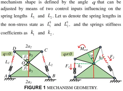
Let us consider first a 1-d.o.f. (degree of freedom) segment of the total flexible structure to be studied, which consists of two rigid triangles connected by a passive joint whose rotation is constrained by two linear springs as shown in Fig. 1. It is assumed that the mechanism geometry is described by the triangle parameters

( , )

a b

and

( , )

a b

, and the

mechanism shape is defined by the angle q that can be adjusted by means of two control inputs influencing on the spring lengths

L

₁ and

L

₂. Let us denote the spring lengths in the non-stress state as

L

0₁ and

L

0₂，and the springs stiffness coefficients as

k

1 and

k

2. 2a1 2a2 b1 b2 L1 _L 2 Mext F1 F2 q h1 h2 A B D _C O q=0 q 0 β1 β2

FIGURE 1 MECHANISM GEOMETRY.

To find mechanism configuration angle qcorresponding to given control inputs

L

0₁ and

L

0₂, let us derive the static equilibrium equation. The forces

F

₁,

F

₂ generated by the springs can be obtained from Hook’s law as follows.

0 0

1 1

(

1 1

);

2 2

(

2 2

)

F



k L



L

F



k L



L

(1) where

L

₁ and

L

₂ are the spring lengths AD , BC

corresponding to the current value of the angle q. These values can be computed from the triangles AODand BOC using the formulas 2 2 1 1 1 2 1 2 1 2 2 2 2 1 2 1 2 2 ( ) 2 cos( ) ( ) 2 cos( ) L c c c c L c c c c           (2) where 2 2 1 1 1 c  a b ; 2 2 2 2 2

c  a b , and the angles



1 ,



2 are expressed via the mechanism parameters as follows

1 12 q







 ;



2 



12q;

 

12

atan( / ) + atan( / )

a b

1 1

a b

2 2 The torques

M

1

 

F h

1 1,

M

2

  

F h

2 2 created by the

forces

F

1,

F

2 in the passive joint O can be computed using the

triangle area relations

L h

_{1 1}



c c

_{1 2}

sin( )



₁ ,

L h

_{2 2}



c c

_{1 2}

sin( )



₂ of AOD and BOC, which yield the following expressions

0 1 1 1 1 1 1 2 1 0 2 2 2 2 2 1 2 2 ( ) (1 ( )) sin( ) ( ) (1 ( )) sin( ) M q k L L c c M q k L L c c           (3)

where the difference in signs is caused by the different directions of the torques generated by the forces

F

1,

F

2 with

respect to the passive joint.

Further, taking into account the external torque

M

_ext applied to the moving platform, the static equilibrium equation for the considered mechanism can be written as follows

1

( )

2

( )+

ext

0

M q



M q M



(4)

Solving this equation we can get the rotation angle

q

₀

corresponding to the control inputs

L

0₁,

L

0₂and to the external torque

M

_extapplied to the moving platform. It is clear that this equation is highly nonlinear and cannot be solved analytically, so it is reasonable to apply the numerical Newton technique, which leads to the iterative scheme





1 ( ) ( ) k k k k ext q  q  M q M M q (5) where

M q

( )



M q

₁

( )



M q

₂

( )

, M q( k)dM q dq

 

. STABILITY ANALYSIS OF THE MECHANISM

Let us now evaluate the stability of the considered mechanism at the equilibriums, which shows its reaction to the external disturbances. In general, this property highly depends on the equilibrium configuration defined by the angle q, which satisfies the equilibrium equation

M q

( )



M

_ext



0

. As follows from the relevant analysis, the function M q( ) can be either

monotonic or non-monotonic one, so the single-segment mechanism under study may have multiple stable and unstable equilibriums, which are studied in detail below.

To analyze the mechanism equilibriums, let us consider the torque-angle curves

M q

( )



M q

₁

( )



M q

₂

( )

defined by Eq. 3 and presented in Fig. 2. It is clear that for the monotonic function M q( ) with negative derivative (see Fig. 2a) increase

of the external loading

M

_ext always leads to higher mechanism resistance, so the equilibrium is unique and stable. However, in the non-monotonic case, while increasing the external loading, it is possible to achieve a point where the mechanism does not resist any more and suddenly changes its configuration as shown in Fig. 2b. It is worth mentioning that similar phenomenon can be observed in other robotic mechanisms and is known in mechanics as “buckling” [13]. Hence, in the non-monotonic case, there maybe three solutions of the equilibrium equation (two stables and one unstable).

As follows from the above presented figures, the static equilibrium defined by angle q is stable if and only if the corresponding derivative M q( ) is negative. However, taking

into account possible shapes of the torque-angle curves M q( )

(a) monotonic case: one equilibrium

-Mext

stable area

stable area

(b) non-monotonic case: three equilibriums

-Mext stable area q q stable area untable area untable area In te rn al t o rq u e (N m ) In te rn al t o rq u e (N m )

FIGURE 2 THE TORQUE-ANGLE CURVES AND EQUILIBRIUMS FOR DIFFERENT COMBINATIONS OF MECHANISM PARAMETERS

points, the considered stability condition can be simplified and reduced to the derivative sign verification at the zero point only,

 

₀ 0

q

M q _  (6)

which is easy to verify in practice. It should be noted that here the derivative represent the mechanism stiffness for the unloaded configuration.

To compute the desired derivative for any given q, it is convenient to represent the function

M q

( )

in the following way

 

_{ }

10

_{ }

02 1 2 1 1 1 2 2 2 1 1 2 2 1 L sin 1 L sin M q c c k c c k L





L





     _  _  _  _     (7)

This allows us to express the mechanism stiffness in general case as follows

 

 

 







 



0 0 1 2 1 2 1 1 1 2 2 2 2 2 0 2 2 0 2 2 1 1 1 2 2 3 3 1 2 1 1 1 2 2 2 1 2 1 2 2 1 1 ( ) M q L L L L c c k cos c c k cos c c k L c c k L sin si L L n                       _{ }        (8)

For the special cases, when q0 and

q





12 (or

q

 



12),

the above expression is simplified respectively to

 





 





0 0 1 1 2 2 1 2 12 1 2 12 2 2 2 0 0 12 1 2 1 1 2 2 1 0 2 3 ( )_q c c cos k k k L k L sin c c k M q L L L k L                     (9)













1 0 2 0 1 1 2 1 12 12 0 2 2 2 0 2 12 1 2 2 1 2 1 1 2 2 3 1 1 2 1 2 2 2 ( 1 )_q c c k cos L L sin c c k c c k L c c M q L L   _                         (10) where

 

2 2 1 2 2 1 1 21 2cos 2 L   c c  c c 





2 2 1 2 2 2 1 1 2 1 cos 2 2 2 L   c c  c c  .

Let us also consider in detail the symmetrical case, for which

a

₁



a

₂,

b

₁



b

₂,

c

₁



c

₂,

k

₁



k

₂ ,

L

0₁



L

0₂. In this case, we can omit some indices and present the torque-angle relationship as well as the stiffness expression in forms that are more compact

 

0 12

12

2 cos sin cos sin

2 2 q M q  ck c_  qL  _   (11) 0 12 12

2 cos cos cos cos

2 2 ( ) M q ck_ c  qL  q   _  (12)

where the control input must satisfy the condition

0



L

0



2

b

, which follows from the mechanism geometry (Fig. 1). To distinguish the monotonic and non-monotonic cases presented in Fig. 2, let us compute the derivative for the unloaded equilibrium configuration q0，which after simplification

can be expressed in the following way









0 2 2 0

2

( )

_q

M q



_



k

b



a



L b

(13)

The latter allows us to present the condition (6) of torque-angle curve monotonicity as 2 0 2 1 L a b b  _{ }   _ _{ } _     (14)

and separate the parameter plane in two regions as shown in Fig. 3a. As follows from this figure, the unloaded equilibrium is always stable if ab. Otherwise, to have a stable unloaded equilibrium, the control inputs

L

₁o



L

o₂ should be higher than certain value

 

2

2 1

;

1, 2

o i

L



b



_



a b



_

i



Non-monotonic L0_/b q q (a) L0/b q q (b) a/b a/b Non-monotonic Energy Torque Torque Energy Monotonic Monotonic

FIGURE 3 STABLE AND UNSTABLE REGIONS OF THE PARAMETER PLANE FOR UNLOADED EQUILIBRIUM q0.

The monotonic and non-monotonic cases are also illustrated by Fig. 3b, which includes the energy curves





2 2 ₀ 1

1

( )

( )

2

i i

E q





_

k L q



L

as the function of the rotation angle q. As follows from this figure, the energy E q( ) has either a single minimum q0

corresponding to a stable equilibrium, or two symmetrical minima





0 2 2

2 arccos

2

e

L b

q

b

a









 



_







(15)

and a local maximum q0 corresponding to two stable equilibriums and one unstable equilibrium.

For the symmetrical case, where

L

₁0



L

0₂, let us also compute the torques (7) at the boundary points

q

 



12.









12 0 2 2 2 2

2

2

( )

_q

abk

M q

L c

b

a

a

b

 





_





(16)

which allows us to decide if the stable equilibriums in the non-monotonic case are located inside of the interval of feasible rotation angles q 





12,



12



. It can be proved that the relevant condition can be expressed as follows



2



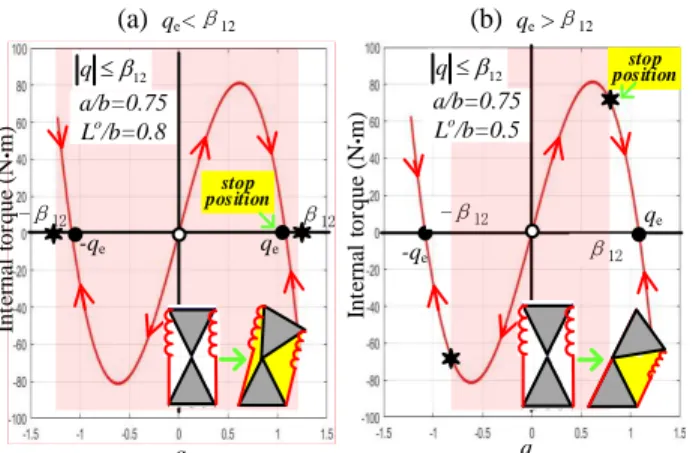
0 2 2 2 2 b a L b a    (17)

and allows user to estimate if the energy minimum is achieved inside or on the border of the feasible region of q. A physical interpretation of this equation is shown in Fig. 4, where two cases are presented. In the first case, the mechanism is unstable in the desired configuration q=0 and jumps to one of two possible stable configurations q q_e that are located inside

of mechanical limits. In the second case, the mechanism is also

unstable in the equilibrium configuration q=0 but it jumps to one of the mechanical limits q ₁₂ (because the stable

configurations are out of the limits). So, a static error appears in both cases, where q is equal to either ₁₂ or q_e. For this

reason, it is necessary to avoid in practice the parameters combinations producing non-monotonic torque-angle curves.

It is also useful to investigate the case when the control inputs are not equal, i.e.

L

₁0



L

0₂, assuming that they produce the desired stable configuration with the output angle q0. In

this case, the torque and its derivative can be presented as follows.

 

0 12 0 12

12 1 2

2 cos sin sin sin

2 2 q q M q ck_ c  qL   L   _   (18)





0 0 0 0 2 2 1 2 1 2

2

cos

cos

sin

)

2

2

(

2

2

L

L

q

L

L

q

k

b

a

q

b

M q





_











a







_



(19) where all notations are the same as in the above expressions (7) and (8). It can be proved from the equilibrium equation that the control inputs

L

0₁,

L

0₂ insuring the desired output angle q

must satisfy the linear relation

0 12 0 12

1

sin

2

sin

2 cos

12

sin

2

2

q

q

L







L







c



q

(20)

which gives infinite set of control variables



0 0



1, 2

L L that may correspond either to stable or unstable equilibrium. To analyze sign of the derivative

dM q dq

( )

, let us consider separately two cases: ab and ab. In the first case, when ab

and mechanism geometry impose the constraint q 



2, all three terms of (19) are negative, so the desired equilibrium configuration q is stable.

q q -β12 β12 -β12 β12 (a) qe<β12 (b) qe >β12 qe -qe qe -qe 12 q q12 a/b=0.75 Lo/b=0.8 a/b=0.75 Lo/b=0.5 stop position stop position Int er na l t or que ( N m ) Int er na l t or que ( N m )

FIGURE 4 LOCATION OF STABLE “●” AND UNSTABLE “O” EQUILIBRIUMS WITH RESPECT TO GEOMETRIC BOUNDARY





 

12, 12



.

In the second case, when ab, the equilibrium maybe either stable or unstable. Corresponding separation curves can be found from the conditions

M q

( ) 0



and

dM q dq

( )



0

, which yield the following system of linear equations with respect to

L

0₁,

L

0₂





0 0 2 2 1 2 0 0 12 12 1 2 12

sin cos sin

sin sin 2 c cos 2 c os si os 2 2 2 2 n 2 2 2 2 2 2 a q q b q a q b q L L b a q L L q c q









_

 _  _ _  _{  }         _  _           (21) whose solution allows us to present the stability condition in the following form

0 3 3 1 0 3 3 2 2 cos sin 2 2 2 cos sin 2 2 L b a a q q b a b b L b a a q q b a b b     _  _  _        _  _  _    (22)

It is worth mentioning that in the case of q0 the above

expressions give the stability condition Eq. 22.

Hence, to achieve the desired configuration q, it is necessary to apply the control inputs

L

₁0,

L

0₂ satisfying both the equilibrium condition Eq. 20 and the stability conditions Eq. 22. Corresponding regions of

L

0₁,

L

0₂ are presented in Fig. 5, which clearly shows for which combination of inputs the desired configuration can be reached geometrically and it is statically stable, and where the angle

q

is constrained by the geometry conditions:









2atan , 2atan , q a b a b q  a b a b      (23) CONCLUSION

The paper presents some results on the stiffness analysis of a new type of tensegrity mechanism, which is composed of two rigid triangles connected by a passive joint. In contrast to conventional cable driven mechanisms, here there are two length-controllable elastic edges that can generate internal preloading. So, the mechanism can change its equilibrium configuration by adjusting the control inputs length. Such design is very promising and convenient for constructing a multi-section serial structures with high flexibility, which are needed in many modern robotic applications.

For this mechanism, the main attention was paid to a symmetrical structure composed of similar triangles. In particular, the case of equal control inputs was investigated in detail and analytical condition of equilibrium stability was obtained, which allows user to select the control inputs ensuring the mechanism controllability. The relation between the external torque and the deflection was also obtained allowing to find loaded equilibriums. It was proved that depending on parameters combinations, the actuation can lead to either the desired mechanism configuration (corresponding to a stable equilibrium) or undesired configuration corresponding to shifted stable equilibrium or joint limits. Besides, similar analysis has been done for the case of non-equal control inputs, and equivalent serial structure was proposed where the passive joint was replaced by a virtual actuated joint with variable stiffness. In future, these results will be used for the stiffness analysis of multi-section mechanisms that may demonstrate unusual behavior under static load and suddenly change its configuration.

ACKNOWLEDGEMENTS

This work was supported by the China Scholarship Council ( No. 201801810036 )

stable non-reachable non-reachable unstable stable unstable non-reachable non-reachable (a) (b) q= -π/3 stable stable q= -π/6 (c) (d)

Fig. 5 Regions of equilibrium stability for different inputs

L

0₁,

L

0₂.

REFERENCES

[1] Rolf, M., & Steil, J. J. (2012, October). Constant curvature continuum kinematics as fast approximate model for the Bionic Handling Assistant. In 2012 IEEE/RSJ International Conference

on Intelligent Robots and Systems (pp. 3440-3446). IEEE.

[2] Yang, Y., & Zhang, W. (2015, December). An elephant-trunk manipulator with twisting flexional rods. In 2015 IEEE

International Conference on Robotics and Biomimetics (ROBIO)(pp. 13-18). IEEE.

[3] Skelton, R. E., & de Oliveira, M. C. (2009). Tensegrity

systems(Vol. 1). New York: Springer.

[4] Moored, K. W., Kemp, T. H., Houle, N. E., & Bart-Smith, H. (2011). Analytical predictions, optimization, and design of a tensegrity-based artificial pectoral fin. International Journal of

Solids and Structures, 48(22-23), 3142-3159.

[5] Duffy, J., Rooney, J., Knight, B., & Crane III, C. D. (2000). A review of a family of self-deploying tensegrity structures with elastic ties. Shock and Vibration Digest, 32(2), 100-106. [6] Arsenault, M., & Gosselin, C. M. (2006). Kinematic, static and

dynamic analysis of a planar 2-DOF tensegrity

mechanism. Mechanism and Machine Theory, 41(9), 1072-1089.

[7] Furet, M., Lettl, M., & Wenger, P. (2018, July). Kinematic analysis of planar tensegrity 2-X manipulators. In International

Symposium on Advances in Robot Kinematics (pp. 153-160). Springer, Cham.

[8] Furet, M., & Wenger, P. (2018, August). Workspace and cuspidality analysis of a 2-X planar manipulator. In IFToMM

Symposium on Mechanism Design for Robotics (pp. 110-117).

Springer, Cham.

[9] Arsenault, M., & Gosselin, C. M. (2006). Kinematic, static and

dynamic analysis of a planar 2-DOF tensegrity

mechanism. Mechanism and Machine Theory, 41(9), 1072-1089.

[10] Wenger, P., & Chablat, D. (2018). Kinetostatic analysis and solution classification of a planar tensegrity mechanism. In Computational Kinematics (pp. 422-431). Springer, Cham. [11] Moon, Y., Crane, C. D., & Roberts, R. G. (2012). Position and

force analysis of a planar tensegrity-based compliant mechanism. Journal of Mechanisms and Robotics, 4(1).

[12] Venkateswaran, S., Furet, M., Chablat, D., & Wenger, P. (2019, August). Design and analysis of a tensegrity mechanism for a bio-inspired robot. In ASME 2019 International Design Engineering Technical Conferences and Computers and Information in Engineering Conference. American Society of Mechanical Engineers Digital Collection.

[13] Jones, R. M. (2006). Buckling of bars, plates, and shells. Bull Ridge Corporation.