R´epublique Alg´erienne D´emocratique et Populaire
Minist`ere de l’Enseignement Sup´erieur et de la Recherche Scientifique Universit´e Mohamed Khider Biskra
N◦ d’ordre :. . . .. S´erie :. . . .
Facult´e des Sciences Exactes et des Sciences de la Nature et de la Vie D´epartement d’Informatique
TH`
ESE
Pr´esent´ee pour obtenir le grade de
DOCTORAT EN SCIENCES EN INFORMATIQUE Par
Hammadi BENNOUI
THEME
Distributed Causal Model-based Diagnosis:
An Approach by Interacting Petri Nets
Soutenue le : 19 Janvier 2012 Devant le jury compos´e de :
M. Djamel Eddine Saidouni Professeur `a l’Universit´e de Constantine Pr´esident M. Allaoua Chaoui Professeur `a l’Universit´e de Constantine Rapporteur M. Kazar Okba Professeur `a l’Universit´e de Biskra Examinateur M. Cherif Foudil Maˆıtre de conf´erences A `a l’Universit´e de Biskra Examinateur M. Mustapha Bourahla Maˆıtre de conf´erences A `a l’Universit´e de M’sila Examinateur M. Kamel Barkaoui Professeur au CNAM de Paris, France Invit´e
Acknowledgment
I would like to thank all the people that supported me in many ways, making possible this work.
First and foremost I want to thank Allaoua Chaoui and Kamel Barkaoui, my supervisors, for their support and their encouragement. I felt so lucky to work with them, not only for their deep knowledge and expertise, but because they are so beautiful people. This thesis is the result of the work done together.
Special thanks to Mourad Maouche and Mohamed Bettaz who introduced me in the field of model-based diagnosis and Petri nets.
Finally, I would like to thank Djamel Eddine Saidouni, Kazar Okba, Cherif Foudil and Mustapha Bourahla for reviewing and evaluating this thesis.
Contents
1 Introduction 1
I
State of the art
7
2 Model-based diagnosis 8 2.1 Introduction . . . 8 2.2 Problem formulation . . . 10 2.2.1 System model . . . 11 2.2.2 Observation . . . 11 2.2.3 Diagnoses . . . 12 2.2.4 Notations . . . 13
2.3 Approaches to model-based diagnosis . . . 14
2.3.1 Consistency-based diagnosis . . . 15
2.3.2 Abductive diagnosis . . . 19
2.3.3 The integration approach . . . 21
2.4 What’s in BM ? . . . 22
2.5 Characterizing diagnostic problems . . . 24
2.6 Solving diagnostic problems . . . 26
2.7 Computational aspects . . . 29
2.8 Conclusion . . . 31
3 Diagnosis within Petri nets 33 3.1 Introduction . . . 33
3.2 Petri nets: Outline . . . 34
3.3 Modeling diagnosis with PNs . . . 35
3.3.1 Fault representation . . . 36 3.3.2 Observation . . . 37 3.3.3 Diagnosis of DES . . . 38 3.4 Diagnosis methods . . . 38 3.4.1 Diagnoser . . . 39 3.4.2 PN unfolding . . . 40
3.4.3 PN backward reachability analysis . . . 42
3.5 Architecture of DES diagnosis . . . 47
3.5.1 Centralized diagnosis . . . 48
3.5.2 Decentralized diagnosis . . . 48
3.5.3 Distributed diagnosis . . . 51
3.6 Conclusion . . . 53
II
Contributions
54
4 A distributed model-based diagnosis 55 4.1 Introduction . . . 554.2 Problem statement . . . 56
4.3 The diagnosis of one agent . . . 57
4.4 The diagnosis of multiple agents . . . 58
4.5 Conclusion . . . 60
5 A distributed BW analysis 62 5.1 Introduction . . . 62
5.2 The system model . . . 63
5.3 A distributed diagnostic reasoning scheme . . . 66
5.3.1 A distributed BW-Analysis . . . 66
5.3.2 A protocol for the distributed BW-Analysis . . . 69
6 A distributed P-invariant analysis 72
6.1 Introduction . . . 72
6.2 Local diagnosis by analyzing P-invariants . . . 73
6.3 Protocol for distributed P-invariant analysis . . . 77
6.4 Conclusion . . . 81
7 Relationships among manifestations 82 7.1 Introduction . . . 82
7.2 Relationships model . . . 83
7.3 Extending the BW-Analysis technique . . . 83
7.4 Extending the P-invariant technique . . . 86
7.4.1 Adaptation of the relationships model . . . 86
7.4.2 Diagnosis by P-invariant analysis . . . 87
7.5 Inconsistent markings . . . 90
7.6 Conclusion . . . 91
List of Figures
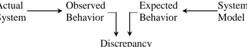
2-1 Diagnosis as the interaction of observation and expectation. . . 12
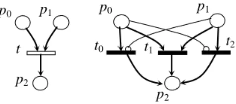
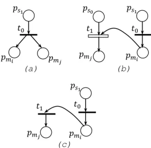
3-1 Or-transition and its semantics. . . 44
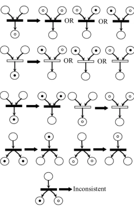
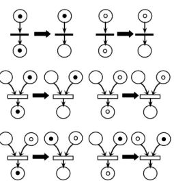
3-2 Backward firing rules. . . 47
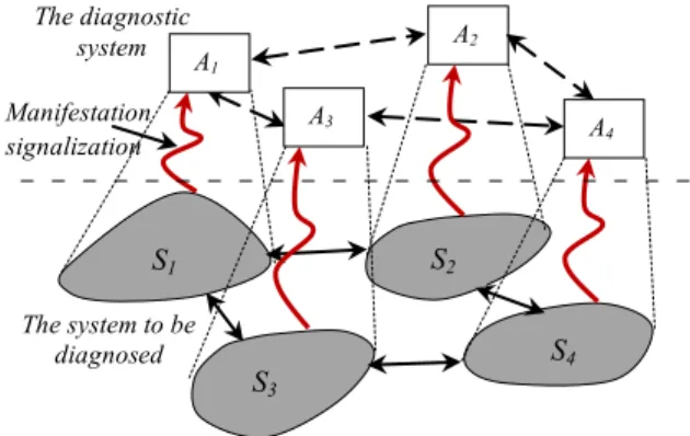
4-1 A diagnostic system architecture. . . 55
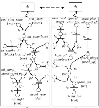
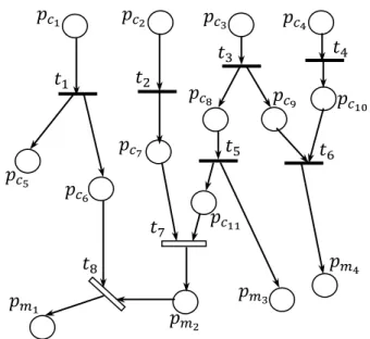
5-1 Example of a distributed BPN. . . 65
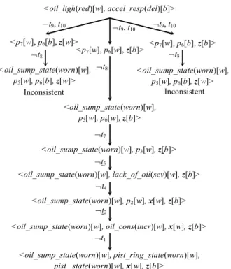
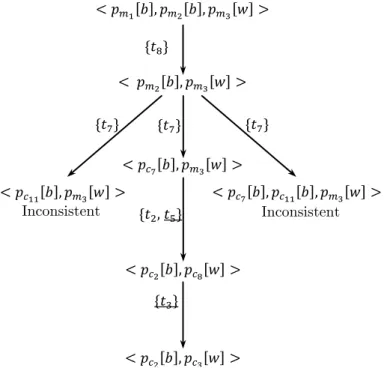
5-2 The BW graph of A1. . . 68
7-1 Relationships that may exist between manifestation instances. . . 84
7-2 Backward firing rules taking into account relationships among manifestations. 85 7-3 Example of a BPN model with relationships among manifestations. . . 86
7-4 The BW graph of Figure 7-3 model. . . 87
7-5 A refined model of relationships among manifestations. . . 88 7-6 A refined example of a BPN model with relationships among manifestations. 89
Chapter 1
Introduction
The problem of fault diagnosis of artifact systems has received a great attention during the last two decades due to its importance in terms of safety and efficiency of operation. Numerous complementary approaches have been proposed, based on the level of detail chosen for the model of the system to be diagnosed and the kinds of faults that need to be diagnosed. The starting point of these approaches is to model the structure and/or behavior of the system to be diagnosed. When an abnormal behavior of the system is observed, the diagnosis consists to tracking back on the model for explaining such a misbehavior. Accordingly, a traditional diagnostic system can be viewed as a centralized system having a model of the whole system to be diagnosed and receiving all observation signalizations. There are, however, several reasons why in some applications such a single agent approach may be inappropriate. First of all, if the system is physically distributed and large, e.g. modern telecommunication networks, there may be not enough time to compute a diagnosis centrally and to communicate all observations. Secondly, if the structure of the system is dynamic, e.g. AGV systems driving in a platoon, it may change too fast to maintain an accurate global model of the system over time. Finally, sometimes a central model is simply undesirable. For example, if the system is distributed over different legal entities, one entity does not wish other entities to have a detailed model of its part of the system. For such systems, a distributed approach of multiple diagnostic agents might offer a solution.
different ways1 (cf. [79]):
• spatially distributed : knowledge of system behavior is distributed over the agents ac-cording to the spatial distribution of the system’s components, and
• semantically distributed : knowledge of system behavior is distributed over the agents according to the type of knowledge, e.g. a separate model of the electrical and of the thermodynamical behavior of the system.
For both types of distributions, a multiagent system can establish the same global diag-noses as a single diagnostic agent having the combined knowledge of all agents [76].
We focalize ourselves in this thesis to the problem of spatially distributed causal model-based diagnosis. We consider the system to be diagnosed as a collection of interacting subsystems in which when a fault occurs in one subsystem, it may generate some fault indications (i.e. symptoms) and may propagate to the neighborhood. The diagnostic system itself is defined as a set of diagnostic agents each of which is associated with a specific subsystem. In particular, each agent has a local model of the assigned subsystem and may receive observations generated only by elements of this subsystem. The local model describes the causal behavior of the subsystem as well as its interactions within adjacent ones. When agents observe an aberrant behavior, each one is charged to explain the received local observation on the basis of its local model. As a result, each diagnostic agent calculates a set of local diagnoses. In causal models, the diagnoses are to be given in terms of initial states that explain the set of observed symptoms using the cause-effect relationships described in the model. Such initial states represent the initial perturbations leading the system to behave abnormally.
Since each agent has a limited knowledge about the whole system to be diagnosed, it may be possible that local diagnoses of different agents are inconsistent when they are considered altogether. In order to ensure the required consistency and to guarantee that such local diagnoses recover completely global ones that would be obtained by a centralized agent having a global view of the whole system, agents should communicate among them to reject inconsistent diagnoses.
We use in this thesis a particular class of Petri nets called “Behavioral Petri Nets” (BPNs) which has been proposed in [2] to represent the causal behavior of a system for centralized diagnosis purposes. In particular, the causal behavior of each subsystem is described by a local BPN model and interactions among subsystems are captured through tokens that may pass via common bordered places between BPNs. Diagnostic reasoning scheme may be accomplished by exploiting classical analysis techniques of Petri nets. More particularly, diagnosis can be implemented locally by a backward analysis (BW-Analysis) of the corre-sponding reachability graph to explain the received local observation. The BW-Analysis exploits two different types of tokens (normal and inhibitor tokens) aimed at modeling the truth or falsity of the condition associated with a marked place. This allows as to point out inconsistencies when looking for possible explanation of a given marking in a BPN. As a result, each agent obtains a set of local initial markings from which diagnoses have to be given. Then, to achieve the consistency with the local diagnoses of all other agents, each one requests from its neighbors the required marking of its bordered places for each computed diagnosis. At this step, agents receiving such a request will construct their reachability graphs in a forward fashion to check if the requested marking of bordered places is reachable from at least one of their computed initial markings. If so, the local diagnosis from which the exchanged message has been generated is considered globally consistent; otherwise, it is not supported by diagnoses of the neighborhood and consequently it must be discarded.
Accordingly, such reasoning suffers from the so-called state space explosion problem even for small net models. This is due to the utilization of reachability graphs as a basis on which analysis is accomplished especially in the consistency checking phase where several graphs may be constructed by each agent. In order to face such a problem, we may exploit algebraic analysis techniques, known also as invariant analysis, which are shown useful in [4, 67, 68] for improving complexity in centralized diagnostic reasoning based on Petri nets versus reachability graph analysis. In particular, we concentrate in our work on the distributed analysis of P-invariants of the net models which are generated in an off-line manner. More specifically, we require that each diagnostic agent utilizes the set of minimal supports of its P-invariants to implement local preliminary computation as well as to check the required consistency of its local diagnoses with those of the other agents. Thus, the set of minimal
supports of P-invariants may be considered as a pre-compiled structure of the system model on which diagnosis is implemented. The idea of using a compiled structure of the system model to the on-line diagnosis is borrowed from Sampath et al. [77] in their work on discrete event systems (DES) diagnosis. They propose to generate from a finite state automaton describing the system model another automaton termed the Diagnoser which encompasses more information about the system state (i.e. information about the presence or absence of faults). The Diagnoser is used to both test the diagnosability properties of the system and perform on-line monitoring of the system for the purpose of diagnosis which necessitates a synchronization between the Diagnoser and the system model. Thus, the invariant based diagnosis is similar to the Diagnoser approach regarding the off-line pre-compilation of the system model to face the complexity problem during on-line diagnosis. However, several features make our proposals different from that of [77] and others, namely we use causal models in which the observations to be explained are modeled as partial states of the system to be diagnosed and not as observable events of the Diagnoser approach. Similarly, the faults in terms of which diagnoses have to be given are considered as initial states which have no causes in the causal model and not as unobservable transitions adopted in the context of DES diagnosis. Another difference is that we do not require that such a compiled structure will be synchronized with the system model which is one of the key features of the approach of [77] and all its extensions [38, 43, 51]. It is to be noted however that in this thesis we do not treat the question of diagnosability analysis and we concentrate only on how to implement diagnosis by distributed analysis of interacting BPNs.
This dissertation is structured in six chapters divided into two parts: the state of the art and contributions. The state of the art part presents background on model-based diagnosis according to logical points of view as well as Petri nets ones. The contribution part contains our proposals for diagnosing distributed systems by analyzing interacting BPNs.
We begin in the following chapter by formulating the diagnostic problem. The chapter concentrates on the model-based view of diagnosis. It is devoted to synthesize the different works that are made in the field. The attention is focused firstly on logical formalizations and on declarative characterizations; and secondly on procedural aspects that characterize different diagnostic engines.
Chapter 3 surveys diagnosis on Petri nets models. It starts with a brief outline of basic notions related to Petri nets as a model for concurrent systems, then it discusses the problem of DES diagnosis as well as DES diagnostic methods that have prevailed in the literature. The chapter concludes with a classification of DES diagnosis implementations according to topological point of view.
The first chapter of the contributions part (chapter 4) attempts to formalize the notion of distributed model-based diagnosis. It defines the diagnostic system as a multi-agent system that reflects the same network structure of the system to be diagnosed. In particular, the chapter characterizes the diagnosis of each agent in the system as well as the distribution of the process of diagnosis over the different agents of the diagnostic system.
In chapter 5, we show how model-based diagnosis of distributed system can be accom-plished by BPN analysis based on reachability graphs. We start by formalizing the system model as a set of place bordered BPNs each of which model the causal behavior of one subsystem, then we show how the BW analysis of each BPN implements local diagnosis of the associated subsystem based on its causal model. Once local diagnoses are obtained, global consistency between them will be ensured through a cooperation protocol among the diagnostic agents. It is to be noted that a preliminary version of such a distributed technique has been published as a conference paper [6].
Based on the drawbacks of the distributed BW analysis (object of chapter 5), chapter 6 proposes the definition of the invariant based technique as an alternative to implement causal model-based diagnosis of distributed systems. In particular, after characterizing diagnostic solutions by the minimal supports of the nets P-invariants the chapter discusses algorithmi-cally local calculations made by each agent as well as how to exploit such supports during consistency checking phase. The invariant based diagnosis technique has been published in [7].
Chapter 7 considers the problem of relationships that may exist between symptoms. This requires in one hand the expression of such relationships in the system model; and on the other hand the adaptation of the analysis techniques to handle these relations. More par-ticularly, the chapter proposes a novel set of backward firing rules to account for precedence relationships among symptom signalizations. Besides such an adaptation, the chapter
con-siders also the case where some of the signaled symptoms have been lost or suppressed. If so, it may be possible that the given diagnostic problem is inconsistent; and the retained so-lution consists to restore the required consistency to the given problem by slightly changing the given observation so that the problem admits an interpretation model. Some parts of chapter 7 contents have been occurred in [5].
Finally, we conclude the thesis by summarizing what we consider as the main contribu-tions of our work as well as their limitacontribu-tions. Perspective works are identified on the basis of such limitations.
Part I
Chapter 2
Model-based diagnosis
2.1
Introduction
Advances in modern design and manufacturing technology have enabled us to build systems of high complexity. When these systems fail to function correctly, they need to be repaired. The repair process pass necessarily through a diagnosis step for locating those subsystems that are responsible for the observed malfunction.
Since the complexity of diagnosis increases with increasing design complexity, the efficient automation of this task becomes essential and gives rise to an important area of computer science. Especially in the area of artificial intelligence, big efforts have been spent in the attempt to define approaches leading to the automatic diagnosis of broken systems. Such efforts have resulted in the proposition of two fundamentally different families of approaches to diagnostic reasoning [48]. One is based on “heuristic-based ”expert systems, the other is based on “model-based ”ones.
In the first, heuristic-based approaches, one attempts to codify diagnostic rules of thumb and past experience of human diagnosticians considered experts in the involved domain. Representatives of these approaches are Expert Systems of the First Generation, with the blood infection diagnosis system MYCIN [80] as the famous instance. Here, diagnostic skills are captured by sets of more or less direct associations between observable symptoms and diseases as their potential causes. Being grounded in experience gained in previous cases, diagnosis was treated as collecting empirical evidence for the presence of certain malfunctions
rather than a strict deduction process. The necessity to state diagnostic knowledge in terms of explicit symptom-fault associations inherently limited the scope of applicability. Only the identification of previously encountered faults was possible based on previously observed symptoms of systems that are well experienced to allow for the enumeration of the relevant associations. Because these associations tend to be quite specific for narrow types of systems, building such systems was a matter of time-consuming single-piece production [31, 48].
All this turned out to be too restrictive when confronted with requirements in diagnosis of technical systems. Industrial application of automated diagnosis has to cover the detec-tion and localizadetec-tion of new kinds of faults, exhibited by newly designed and constructed systems and the interpretation of symptoms never observed before. The diagnosis of such systems stems from knowledge about the physical and technological principles underlying the (intended or deviating) functioning of these systems which allows one to systematically deduce fault hypotheses from available observations even if the system is novel.
The key idea of the second family of approaches to diagnosis, often called diagnosis from the first principles or model-based diagnosis, is to explicitly represent this knowledge as a model of the system structure and/or behavior of its constituents and to organize diagnosis as an inference process based on this model and the observed behavior. This view created the demand for and the possibility of developing a rigorous theoretical foundation for automated diagnosis. In particular, this comprises a formal characterization of the goal and of the inferences that achieve the goal, given model-based predictions and the actual observations of the system’s behavior. Early introduced, model-based diagnostic systems, referred to as Second Generation Expert Systems such as those proposed in [27, 28, 74], provide declarative system-independent representation languages and system-independent diagnostic procedures. As a consequence of this independence, they are capable, using hierarchical representations [58], of diagnosing complex systems in any domain. Moreover, they are more robust than heuristic-based systems, because they can deal with unexpected cases not covered by heuristic rules. In addition, their knowledge bases are less expensive to create and flexible in regard to design changes since they are a straightforward representation of designs. They do not require rule verification, which can be serious problem in writing heuristic rules. However, the drawback of model-based diagnostic systems is that they require
more complex computation, and hence they are generally not efficient as heuristic-based ones which can guide efficient diagnosis for known cases.
Different attempts to combine heuristic-based and model-based approaches have been made by some researchers [20, 33, 48]. The searched goal in these works consists to get benefit of the advantages of both approaches, namely the robustness of model-based reasoning in one hand and the simplicity of computation and efficiency characterizing heuristic-based one at the other hand.
The overall goal of this chapter is to survey the foundations of model-based diagnosis. In a little more than twenty years, work on automated diagnosis based on models has managed both to establish a strong theoretical basis and to create a technology mature enough to tackle real industrial applications. This does not only allow us to build application systems with formally stated preconditions and provable capabilities and properties. It also provides challenges for theoretical work and hard criteria for evaluating its results and helps to focus it. In fact, model-based diagnosis becomes really one of the rare success stories in artificial intelligence [31].
We begin, in the following section by presenting a formulation of the diagnostic problem within a model-based reasoning view. It introduces some notations that will be used to present, in section 2.3, the main diagnostic approaches that have prevailed in the literature, namely: consistency-based and abductive approaches to diagnosis. A unified approach which integrates these two approaches is outlined. Details concerning the content of the model of the system to be diagnosed are presented in section 2.4. Section 2.5 and 2.6 give the logical characterization of the diagnostic problem and of the set of solutions to such a problem. Procedural aspects of the inference mechanisms proposed in different diagnostic systems are synthesized in section 2.7. Finally, section 2.8 summarizes the main concepts presented in this chapter.
2.2
Problem formulation
Starting with the logical framework given in [74], we make use, in this section, of the first-order logic with equality as a language of knowledge representation.
2.2.1
System model
Unlike the heuristic-based approaches to diagnosis, model-based approaches are proposed to diagnose broken systems independently of the application domain. That is why, a gen-eral domain-independent concept of a system description is indispensable. The following definition of a system description introduced by Reiter in [74] has been considered by most model-based diagnostic frameworks. It is designed to formalize as abstractly as possible the concept of a component, and the concept of a collection of interacting components.
Definition 1 A system description SD for a system S is a pair (BM , COM P S), where: 1. BM , the behavioral model, is a set of first-order formulas representing the knowledge
about S;
2. COM P S, the system components, is a finite set of constants.
In all intended applications, the behavioral model will mention a distinguished unary predicate AB(.), interpreted to mean “abnormal ”. The argument of such a predicate neces-sarily belongs to COM P S. However, as mentioned in [74] it is possible to introduce several kinds ofAB(.) predicates and represent more general component properties.
The use of AB predicate for describing a system is borrowed from McCarty [55] who exploits such a predicate in conjunction with his formalization of circumscription to account for various patterns of nonmonotonic common-sense reasoning.
2.2.2
Observation
Real-world diagnostic settings involve observations (or measurements). Without observa-tions, we have no way of determining whether something is wrong and hence whether a diagnosis is called for.
Definition 2 (from [74]) An observation OBS for a system S is a finite set of first-order formulas defining I, the inputs, and O, the outputs of S.
Notice that distinguished inputs and outputs are features of many man-made artifacts, such as electronic devices. In other applications, however, the observation OBS may not
define a set of inputs. It specifies only a set of findings as observable elements of the system to be diagnosed.
It should be also noted that OBS does not specify all outputs of the system S, nor that SD is a complete description (the behavior of each component is not assumed to be completely specified). The only assumption in most diagnostic frameworks is that the given knowledge is consistent. In other words, (BM ∪ OBS) admits a particular model, the so-called intended interpretation [32], which represents the actual problem universe.
2.2.3
Diagnoses
Suppose that we have determined that a system S = (BM, {c1, ..., cn}) is faulty, by which we mean informally that we have made an observation OBS which conflicts with the way the system is meant to behave if all its components behave correctly.
The repair of S will pass necessarily through a diagnosis step for explaining the observed malfunction. It consists to find a subset of components – say, ∆ ⊆ COM P S – which, when assumed to be failed, will explain why the system exhibits a misbehavior. Thus, a diagnosis can be defined intuitively as a conjunction that certain of the components are faulty and the rest normal. Now the main problem is to specify which components we conjuncture to be faulty in order to provide an explanation for the observed malfunction.
To reach such specification, a model-based diagnosis is guided by the interaction be-tween observations and predictions conducted separately from the system model (Figure 2-1). Thus, it relies solely on the system model BM , its components COM P S, and the observation OBS. In particular, it does not use any heuristic information about the system failures gained by the experience, for example, of the kind “when the system exhibits such and such aberrant behavior, then in 90% of these cases, such and such components have failed”. System Model Actual System Observed Behavior Expected Behavior Discrepancy
2.2.4
Notations
When computing diagnoses, we are interested in discovering formulas where AB is the only predicate symbol which occurs. Therefore, let LAB be a first-order language which contains all the formulas which we can built with theAB predicate symbol alone.
Notation 1 A formula (respec. clause, respec. conjunction, respec. literal) from the lan-guage LAB is referred to as an ab-formula (respec. ab-clause, respec. ab-conjunction, respec. ab-literal).
Any diagnosis will be represented as an ab-conjunction which does not contain two occur-rences of the same component. In particular, a diagnosis is a satisfiable ab-conjunction. Note that there exists only a finite number of ab-formulas (up to logical equivalence). Moreover, we adopt the following notation:
Notation 2
• The set of components occurring in an ab-conjunction ∆ is denoted by C(∆); • The set of positive literals in ∆ is denoted by ∆+;
• The set of negative literals in ∆ is denoted by ∆−.
The dual concept of prime implicant and prime implicate in first-order logic play a central role in most formalizations of model-based diagnosis. Let us present their definitions [29, 32]. Definition 3 Let Ic be an existentially quantified conjunction of literals, then Ic is an im-plicant of a closed formula F if Ic ` F . Let P Ic be an implicant of a closed formula F , then P Ic is a prime implicant of F if P Ic ` F and, for any purely existential conjunction of literals P Ic0, if P Ic0 ` F and P Ic` P Ic0 then P I
0
c` P Ic.
Definition 4 Let Idbe a universally quantified disjunction of literals, then Idis an implicate of a closed formula F if F ` Id. Let P Id be an implicate of a closed formula F , then P Id is a prime implicate of F if F ` P Id and, for any purely universal disjunction of literals P Id0, if F ` P Id0 and P Id0 ` P Id then P Id` P Id0.
2.3
Approaches to model-based diagnosis
The ultimate objective of the diagnostic reasoning is to determine the state of each compo-nent of the system to be diagnosed. Formally, we have from [27, 28, 29, 74]:
Definition 5 The actual diagnosis, ∆, is an ab-conjunction such that: • ∆ is complete: the state AB(c) or ¬AB(c) of each component c is given; • ∆ holds in the intended interpretation.
Unfortunately, due to the incompleteness of our knowledge about the system, it is not always possible to compute ∆ in a purely deductive way. By deduction only a set of partial diagnoses, ∆j1, ..., ∆jn, is usually generated. The term partial means that the state of all
components is not determined.
Since the actual diagnosis is complete and holds in the intended interpretation1, then ∆ implies any ab-formula that holds in that interpretation. In particular, among the sets of partial diagnoses, there is at least one partial diagnosis ∆ji that can be extended to account
for the state of all components. Formally, we have: ∆ ` ∆ji.
Thus, computing diagnoses turns out to be: 1. selecting some partial diagnoses, and
2. extending them to set the state of a maximum number of components with a maximal confidence.
Once again, this contributes to support the thesis that diagnostic reasoning is by nature hypothetico-deductive [32]. This point of view has leads researchers to define some preference criteria for characterizing the hypotheses that should be assumed when extending partial diagnoses.
Different formalizations of this notion of diagnostic reasoning have been proposed in the literature. The first attempts to such formalizations have generally considered two extremes of the diagnosis problem:
1. There is knowledge about how components are structured and work normally. There is no knowledge as to how malfunctions occur and manifest themselves. Diagnosis consists of isolating deviations from normal behavior. This has normally been the preserve of an approach termed consistency-based diagnosis [23, 27, 74].
2. We have just information on faults (diseases) and their symptoms, and want to ac-count for abnormal observations. This has traditionally been the preserve of a second approach called abduction-based diagnosis [14, 16, 21, 66].
In the following, we attempt to provide the principles of each of these approaches with an emphasize on their preference criteria, then we present a unified definition that will be used throughout this thesis.
2.3.1
Consistency-based diagnosis
Since it is proposed originally to deal with models of the correct behavior, consistency-based diagnosis [23, 27, 30, 74] is oriented towards diagnosing systems with the following requirement: there always exist characteristic manifestations to be observed when the system works normally. The components of systems such as electronic devices meet this feature since the expected outputs of each component can be expressed as a function of its inputs. In this approach, the behavioral model is constructed according to the following methodology [31]:
1. for each component c of COM P S that could be faulty, we have the hypothesis ¬AB(c); 2. we write as facts implications that state what follows from assumptions of normality.
Suppose that S = (BM, COM P S) is a system under diagnosis and let O(I) be the expected outputs of S. This can be formalized by:
BM ∪ I ∪ {¬AB(c) | c ∈ COM P S} ` O(I)
Suppose that there is a discrepancy between O, the observed outputs, and O(I). Then, one can conclude that the system S is behaving incorrectly. Indeed, assume that:
BM ∪ I ∪ {¬AB(c) | c ∈ COM P S} ` (O(I) ⇒ ¬O) Then, necessarily we have:
BM ∪ OBS ∪ {¬AB(c) | c ∈ COM P S} is inconsistent.
As it has noted in [18, 27, 32, 74], the objective of consistency-based diagnosis is to explain this inconsistency which stems from the assumption {¬AB(c) | c ∈ COM P S}, i.e. that all components are behaving correctly.
Consequently, ∆ such that C(∆−) = COM P S is not the actual diagnosis since any presumed diagnosis must be consistent with the given knowledge. A possible diagnosis ∆ for S must be an ab-conjunction such that BM ∪ OBS ∪ {∆} is consistent [27, 29, 31, 32, 74]. Note that such diagnosis contributes to explain why the observed outputs differ from the expected ones when assuming that all components are normal.
Preference criteria
In this paragraph, we present the two preference criteria used in consistency-based diagnosis for refining the set of diagnoses.
A. Maximizing the number of described components
Among the possible diagnoses, the preferred ones are those which set the state of the maximal number of components. Hence, they are exactly the possible ones.
As we have mentioned, in most cases the incompleteness of the knowledge prevents us from obtaining the complete possible diagnoses in a purely deductive way. Hence, obtaining a complete possible diagnosis ∆ generally requires to make additional hypotheses. Formally, if ∆ is a complete possible diagnosis, then according to [74] we have:
BM ∪ OBS ∪ {¬AB(ci) | ci ∈ C(∆−)} ` ∧cj∈C(∆+)AB(cj)
Generally, there are several complete possible diagnoses. Hence, more selection is needed for refining those diagnoses. This calls for the following second criterion.
B. Minimizing the set of abnormal components
Among the complete possible diagnoses, the preferred ones are those including the minimal sets of abnormal components. More precisely, if ∆1 and ∆2 are two complete possible diagnoses and C(∆+1) is a subset of C(∆+2) then ∆1 will be preferred to ∆2.
Thus, if ∆ is a complete possible diagnosis, then ∆ is minimal if among all complete diagnoses, C(∆+) is minimal w.r.t set inclusion.
In fact, the minimality criterion is nothing but it is the formal expression of the parsimony principle proposed in [74]. Probability theory argues in favor of this criterion when for each component the probability of failure is lower than the probability of correct behavior.
Characterizing and computing diagnoses
Our objective in this paragraph is to show how to determine all diagnoses for a malfunc-tioning system and to present a logical characterization of complete possible and minimal diagnoses. There is a direct generate-and-test mechanism based upon the consistency re-quired in this approach: systematically generate subsets ∆ of COM P S, generating ∆s with minimal cardinality first, and test the consistency of
BM ∪ OBS ∪ {¬AB(c) | c ∈ COM P S − ∆}
As it has been noted in most papers of model-based diagnosis, the previous problem with this mechanism is that it is too inefficient for systems with large number of components. Instead, Reiter in [74] proposes a method based upon a suitable formalization of the concept of a conflict, a concept due originally to de Kleer [27].
In [29, 31], a conflict for a diagnostic problem is defined as an ab-clause entailed by BM ∪ OBS. A positive conflict is a conflict all of whose literals are positive. In other words, a positive conflict is a subset C ⊂ COM P S which cannot all be functioning correctly; i.e. BM ∪ OBS ∪ {¬AB(c) | c ∈ C} is inconsistent. More precisely, a conflict is any ab-clause which is an implicate of BM ∪ OBS.
To achieve the set of diagnoses for a broken system, three fundamental subtasks will be explored [24]:
• generating hypotheses by reasoning from a symptom to a positive conflict (i.e. to a collection of components whose misbehavior may plausibly have caused that symptom); • testing each hypothesis to see whether it can account for all observations of system
behavior; then
• discriminating among those that survive testing.
Thus, the concept of conflicts provide an intermediate step in determining the diagnoses and are central to most diagnostic frameworks.
We should now present the following characterization which has been introduced in [29, 32]. It defines the set of complete possible and minimal diagnoses in terms of prime implicants.
Characterization 1 Let DD+ be the set of all positive conflicts of S, the system to be diagnosed. The diagnosis ∆ such that C(∆+) = {cj1, cj2, ..., cjm} is a complete possible and
minimal diagnosis iff AB(cj1) ∧AB(cj2) ∧ · · · ∧AB(cjm) is a prime implicant of DD + . In [29], it has been shown that the minimal complete and possible diagnoses cannot be considered as a basis for describing the complete possible diagnoses. It has also been proved that changing the status of a component from normal to abnormal in a complete possible diagnosis does not necessarily result in a possible diagnosis.
Adequacy of preference criteria
In the consistency-based approach any computed diagnosis does not exactly explain the observed behavior of the system. In fact the observations, uniformly embedded in the rest of the knowledge, only contribute to prove the inconsistency of the system when assuming that all components are normal. In other words, the observed actual behavior is not significant. What is important here is that this observed behavior differs from the expected one. That is why the consistency-based approach leads sometimes to undesirable results as it is illustrated in the domain of digital circuits by [32].
2.3.2
Abductive diagnosis
Abductive diagnosis [14, 16, 21, 66] is proposed originally to deal with fault behavioral models (i.e. models of the faulty behaviors of the system to be diagnosed). It views the world in terms of causes and effects. The methodology followed in this approach is [66]:
1. The possible hypotheses are the possible causes (faults, diseases) parametrized by the values which they depend;
2. We axiomatize how symptoms follow from causes. These axioms should be facts if the symptom is always present given the cause and be possible hypotheses otherwise. Because the correct behavior of the system to be diagnosed is not modeled, its expected outputs cannot be predicted. Hence, it is not possible to detect any discrepancy between the observed outputs and the expected ones. Unlike, the consistency-based approach, in the abductive approach BM ∪ OBS ∪ {¬AB(c)} remains consistent.
Since there is no inconsistency to explain when the expected normal manifestations are unavailable, diagnostic reasoning is confined to giving some account for some observed man-ifestations.
Let CO be a combination of outputs to be explained. The abductive diagnosis for CO is defined to be an ab-conjunction ∆ such that:
• BM ∪ I ∪ ∆ ` CO and
• BM ∪ I ∪ ∆ is consistent; where CO ⊆ O.
Let us present the two preference criteria which are used in this approach to refine the set of diagnoses.
Preference criteria
A. Maximizing the explained outputs
In the abduction-based approach to diagnosis, the selection of preferred diagnoses appeals to the confirmation principle [17]: the preferred diagnoses are those which explain a maximal set
of manifestations. However, not all manifestations are equally significant and an interesting problem is the selection of a pertinent subset of manifestations to be explained.
Clearly, the confidence we have in some abductive diagnosis increases with the number of explained outputs.
B. Minimizing the abnormality
Among the abductive diagnoses for a given combination of outputs CO, the preferred ones are those including a minimum number of abnormal components. In other words, let ∆ be an abductive diagnosis for CO, then ∆ is minimal if among all abductive diagnoses for CO, C(∆) is minimal w.r.t set inclusion.
This time, the probability theory gives evidence for this criterion. Indeed, consider ∆ and ∆0 two abductive diagnoses for CO such that ∆ implies ∆0. By this criterion, we prefer the minimal one ∆0 which is more probable than ∆.
Characterizing and computing diagnoses
In [29, 31], a characterization of the abductive view for diagnosis is provided. It relates also the abductive diagnoses to the notion of prime implicants.
Characterization 2 The abductive diagnoses for CO are exactly the positive implicants of (BM ∧ I) =⇒ CO which are consistent with BM ∪ I. The minimal abductive diagnoses for CO are exactly the positive ab-prime implicants of (BM ∧ I) =⇒ CO which are consistent with BM ∪ I.
Clearly, any abductive diagnosis is an extension of at least one minimal abductive diag-nosis. Nevertheless, not every extension of a minimal abductive diagnosis is an abductive one since this operation can lead to an inconsistency with BM ∪ I.
Adequacy of preference criteria
The main drawback of the abduction-based diagnostic approach, as it is defined above, is the following: the actual diagnosis is not necessarily an extension of a minimal abductive diagnosis. More precisely, any abductive diagnosis is not necessarily a possible one. As in
[32], considering the definition of an abductive diagnosis ∆, one can conclude that BM ∪ I ∪ ∆ ∪ CO is consistent.
Nevertheless, any abductive diagnosis is necessarily a possible when CO = O. In par-ticular, every complete abductive diagnosis for O is a complete possible diagnosis [14, 17]. Unfortunately, as it is shown by [32], an abductive diagnosis for O does not always exist.
As one can easily gather from these presentations, consistency-based and abductive di-agnosis differ in the representation about normality and faults and in the meaning they give to “explain”. Typically, according to the consistency-based view, a component is abnor-mal if its observed behavior deviates from the expected one; while in the abductive view, a component is abnormal if it manifests as it is described in the behavioral model (in fact, BM will describe according to the abductive approach different faulty behavioral modes. In the discussion above we have assumed, for reasons of simplicity, that only one faulty behavioral mode, notedAB, is modeled). The difference of explanation becomes obvious, for the consistency-based diagnosis, a solution explains why the system exhibits a malfunction; while in the abductive one, a solution attempts to explain why the system reacts as it is observed.
2.3.3
The integration approach
In these views of model-based diagnosis, the link between consistency-based reasoning and models of the correct behavior and the one between abductive reasoning and faulty models seem to be a natural choice: if one has a theory (the fault model) that can predict the observations, then the notion of covering is the “right”notion of explanation; while if the observations are only the “negation”of the predictions of the theory (the model of the correct behavior), then consistency is the “right”notion of explanation.
Over the last two decades, some attempts to break such privileged links have been made [17, 28, 32] and the advantages of combining fault models and models of the correct behavior have been recognized by some researchers [17, 18, 66]. The approaches to such a combination can be classified into two main groups [18]:
• extensions of abductive diagnosis to deal with models of the correct behavior [16, 66].
In almost all these approaches the integration is very homogeneous: the correct and faulty behaviors of a system have been represented in a uniform way and very few changes to the original reasoning schemes have been made.
Consequently, Console and Torasso in [18] analyze the two former approaches of diagnosis at their logical definitions. They tried to propose a unified framework based on the integra-tion of consistency-based and abductive reasoning rather than extending one of them. In particular, they single out the existence of a spectrum of alternatives in the logical definition of diagnosis by reformulating each of the two notions of diagnostic problem as an abduction one with consistency constraints. The alternatives in such a spectrum range from purely consistency-based approaches (such as the one proposed by de Kleer and Williams [27]) to purely abductive approaches (such as the one proposed by Poole [66]).
Since this spectrum appears as a general framework, having the two approaches presented above as particular cases, we attempt in the following to describe with more details the principle concepts that characterize this framework. In our proposals presented in the second part, we make adaptation of these concepts for diagnosing multiple failures in distributed systems.
2.4
What’s in BM ?
According to the unified approach outlined above, the set of normal and faulty behaviors of the system to be diagnosed should be described in a uniform way using a suitable language. In this approach, each component of COM P S is characterized by a set of behavioral modes. Such characterization was introduced by Holtzblatt [41] in his generalization of theGDE sys-tem (General Diagnostic Engine) [27] and used by de Kleer and Williams in theirSHERLOCK’s system [28].
In SHERLOCK, the behavior of the system to be diagnosed S can be represented as the consequences of the behavioral modes of its constituents. In particular, each component ci is associated with a set of behavioral modes {correct, f aulti1, ..., f aultin} (where correct
corresponds to a distinguished faulty behavior of the component). Notice that one of such faulty modes could be the “unknown mode”with which no model is associated (see [28]). The union of the sets of behavioral modes of all components of S are denoted by the set of abducible symbols. The reason for such a name will be clear in the following. As we shall see, in fact the fundamental problem of diagnosis is that of determining, given a set of observations, the behavioral modes of the components of S “explaining”the observations. This means that the abducible symbols are the basic elements of such “explanations”. Given an abducible symbol α, the fact that a component c is in mode α is represented by the atom α(c).
Given the behavioral modes of the components COM P S of S and the consequences of such modes, one can build the system description SD which specifies the structure and behavior of S as discussed in [28]. The structure of S specifies the components and their interconnections. Components are described as being in one of the set of its distinct modes, where each mode captures a physical manifestation of the component. The behavior of each component is characterized by describing its behavior in each of its distinct modes.
In [18], the behavioral model BM is formed by a set of Horn clauses in which the set of predicate symbols are partitioned into the two subclasses of the abducible and non-abducible symbols. The abducible symbols do not appear in the head of any clause in BM . This cor-responds to assuming that the behavioral modes of the components are “primitive”concepts (in the sense that they cannot be defined in terms of other concepts).
As a simple example, consider the problem of modeling the behavior of a digital circuit containing and-gates [40]. Let us assume that we distinguish three different behavioral modes of an and-gate, i.e. that its set of behavioral modes is {correct, stuck at 0, stuck at 1}; the behavioral model of the circuit will contains the formulae:
and gate(X) ∧ correct(X) ∧ inp1(X, X1) ∧ inp2(X, X2) −→ out(X, fAN D(X1, X2) and gate(X) ∧ stuck at 0(X) −→ out(X, 0)
and gate(X) ∧ stuck at 1(X) −→ out(X, 1)
where fAN D(X1, X2) is the logical AN D of X1 and X2. Notice that {correct, stuck at 0, stuck at 1} is the set of abducible symbols in such a model and those conditions which appear only in the body of a clause in BM and which are not abducibles (such as, for
example, inp1 and inp2) may correspond to contextual conditions; we shall return more precisely to this point in the next section.
In the discussion above, BM is assumed to describe a model of the structure and behavior of the system to be diagnosed. However, all the discussion can be applied also to the case where the structure is not modeled at all and BM is a “causal model ”of the behavior of the system under diagnosis. Causal models have been widely adopted in model-based diagnosis since the work of Weiss et al. in CASENET[89] and Patil in ABEL [61].
In causal models, the behavior of a system is characterized by a set of states (in fact, partial states, that is, entities that partially describe a situation in which the modeled system can be at a given time); each of which is in turn characterized by a finite set of admissible values, and relations among these states (i.e. cause-effect transformations among instances of states). For diagnostic purposes, [16] indicates that it is useful to distinguish among at least three types of states in the model:
• Initial states: they correspond to states which have no causes in the model. In the case of an abnormal behavioral model, they represent the initial perturbations leading the system to a given malfunction; and thus, they define the set of abducible symbols; • Internal states: corresponding to the consequences of initial states. They are attached to system components that are not susceptible to make a part of a diagnosis, because they can be explained by the elements of initial states;
• Manifestations: corresponding to observable or measurable states and thus represent-ing all expected symptoms in the case of faulty models.
In this view, performing a diagnosis means to explain a set of manifestations in terms of initial states, using the cause-effect relationships described in the model.
2.5
Characterizing diagnostic problems
In [18], the authors analyze in detail the notion of diagnostic problem. They argue that it is characterized by different types of data which must be treated in very different way in the diagnostic process.
In particular, a major distinction that they introduce is the one between contextual data and observations (such distinction has been originally proposed in [73] where the term “setting factor”is used to denote contextual data).
Contextual data are a set of parameters providing (contextual) information about the specific case under examination; typical examples are data such as the sex or the age of a patient (in medical diagnosis) or the “inputs”to a device (in other applications). Such data are very important since they allow the diagnostician to make predictions about the behavior of the system to be diagnosed (for example, the fact that a patient is a male allows a physician to exclude certain pathologies and to focus on other pathologies [18]). Typically, contextual data are known when a case is analyzed (or they can be easily gathered) and in some cases they are necessary to characterize the case itself. The important point is that contextual data need not to be accounted for by a diagnosis, but they are rather used to predict the behavior of the system to be diagnosed.
Data corresponding to observations, on the other hand, play a very different role (typical examples of observations are clinical findings or laboratory tests in a medical diagnosis, the outputs of a device in other applications). Observations are data that must be accounted for by a diagnosis. Now, let us present their definition of a diagnostic problem.
Definition 6 A diagnostic problem DP is a triple DP = hhBM, COM P Si, Ctx, OBSi, where:
• hBM, COM P Si is the system description of the system to be diagnosed; • Ctx is a set of ground atoms denoting the set of contextual data;
• OBS is a set of ground atoms denoting the set of observations to be explained.
The meaning of each atom f (a) in Ctx or in OBS is the following: in the specific problem to be solved the value a has been observed for the parameter f.
In this definition, different requirements are imposed by the authors. First, they impose the constraint that Ctx ∪ OBS can contain at most one instance of each symbol (i.e. an observable parameter cannot have more than one value). This corresponds to abstracting from time; i.e. to assuming that diagnosis is performed in a static environment (which is a
common assumption in most formalizations of model-based diagnosis, except some attempts to introduce the notion of time in diagnosis such as the works of [15, 89]). Second, they assume that all pieces of contextual information are known a priori (i.e. they are part of the data). Last, they impose, as it can be remarked from the definition, that contextual data and observations are represented by two distinguished sets of atoms.
2.6
Solving diagnostic problems
As we noticed previously, diagnosis can be characterized as the process of generating “ex-planations”for a set of observations in a given context. However, the term “explanation”has been used in the first model-based diagnostic systems with at least two different meanings (i.e. two different logical notions of “explanation”).
• explanation as consistency (weak notion of explanation); in such a case a diagnosis explains an observation m if it does not contradict m (i.e. if it does not support ¬m); • explanation as covering (strong notion of explanation); in such a case a diagnosis
explains an observation m if it directly support m.
In most of the formalizations of diagnosis proposed in the literature, one of the two al-ternatives has been chosen. However, because the goal of the above characterization is of generalizing the other definitions of model-based diagnostic problem, an abstract definition which embeds the possibility of choosing among the two notions of explanation is indispens-able. The following definition proposed in [18] is based on the reformulation of a diagnostic problem as an abduction problem with consistency constraints. Such reformulation contains a critical step: choosing which observations must be covered by a diagnosis. It is such a con-troversial choice that distinguishes among different definitions of diagnosis (of “explanation”) and allows us to single out a spectrum of definitions.
Definition 7 Given a diagnostic problem DP = hhBM, COM P Si, Ctx, OBSi, an abduc-tion problem AP corresponding to DP is a triple AP = hhBM, COM P Si, Ctx, hΨ+, Ψ−ii, where:
• Ψ+⊆ OBS
• Ψ−= {¬f (x) | f (y) ∈ OBS, for each admissible value x of f other than y}
Ψ+ is the set of observation atoms that must be covered by a solution; in principle, any subset of OBS can be chosen. Ψ− on the other hand, is a set of negative literals and characterizes the set of values which conflict with the observation.
As we shall see, Ψ− is used for consistency checking (Ψ− is a set of denials and is interpreted as a set of consistency constraints that the solutions to the abduction problem must satisfy). Notice that Ψ− may be an infinite set (in case at least one of the observable parameters can assume an infinite set of values).
The previous definitions take the assumption that the observation OBS characterizing a diagnostic problem is a set of atoms. This corresponds to assuming that definite knowledge about the observation is available. In some cases, however, it may be interesting to have the possibility of providing incomplete (partial) descriptions of the data characterizing a diagnostic problem. One way to specify incomplete knowledge about data was exposed in [16]. It consists to provide “negative”information about the observable parameters. Let us consider a negative information ¬f (a): this can be regarded as a way to express that no definite knowledge about the actual value of the parameter f is available, but certainly f does not assume the value a (while any other value might a plausible).
In the following, we shall concentrate on the case where all the observation atoms are positive (definite); however, all the discussion can be easily generalized also to the case where “negative observations”are allowed. The definition of an abduction problem associated with a diagnostic problem can in fact be easily extended with positive (definite) and negative observations. In such a case, the atoms in Ψ+are a subset of the positive observations; while Ψ− is the set of negative literals obtained as the union of the negative observations and the values that conflict with the positive ones.
We can now move to characterize the solutions to an abduction problem. The central task of abductive (diagnostic) reasoning is to identify those behavioral modes of the components whose consequences cover Ψ+(i.e. which predict Ψ+) consistently with Ψ−. More specifically, the space of hypotheses that has to be analyzed in order to determine the explanations for an
abduction problem AP is the space of the assignments of behavioral modes to the components COM P S of the system. In particular, we have the following definition introduced in [28]. Definition 8 Given a system description hBM, COM P Si and given the set of abducible symbols in BM , an assignment W for COM P S is a set of ground abducible atoms such that for each c ∈ COM P S, W contains exactly one element of the form α(c) (where α is an abducible symbol).
Notice that this corresponds to assuming that the behavioral modes of each component are mutually exclusive (which seems to be a reasonable assumption).
In particular, we are interested in those assignments that cover Ψ+consistently with Ψ−. Definition 9 Given an abduction problem AP = hhBM, COM P Si, Ctx, hΨ+, Ψ−ii, an as-signment W for COM P S is an explanation for AP iff
1. W covers Ψ+, that is for each m ∈ Ψ+ we have that BM ∪ Ctx ∪ W ` m
2. W is consistent with Ψ−, that is BM ∪ Ctx ∪ W ∪ Ψ− is consistent. In other words, for each ¬m ∈ Ψ− we have that BM ∪ Ctx ∪ W 0 m
Some remarks are worthwhile on such a definition. First of all, notice that consistency with Ψ− corresponds to not predicting any value for an observable parameter different from the actual one (i.e. conflicting with the observed one). The notion of consistency used in this definition, therefore, is the same used in consistency-based definitions of diagnosis [23, 24, 27, 74]. Thus, this definition combines the two notions of explanation discussed previously: in order to provide a solution to an abduction problem (and thus to a diagnostic problem), an assignment must be consistent with all the observable parameters and must cover a selected group of parameters.
A second remark concerns the role played by contextual data. Such data are used to pre-dict the expected behavior of the system and thus they play a role in consistency checking; however, they do not have to be covered. One way to enforce between contextual data and observations was proposed by Poole [66], who started from a simple example: given a system with input i and output o, how should one represent such data? Poole argued that there are
two alternative logical representations (namely i ∧ o and i −→ o) and that different formal-izations of diagnosis require different representations (more specifically, abductive diagnosis requires the representation of observation as an implication i −→ o; while consistency-based diagnosis requires the representation as a conjunction i ∧ o). Actually, such different repre-sentations can be regarded as a technical way to enforce the different roles played by the different types of data discussed above and captured, at the knowledge level, by the previous definition.
In general, given an abduction problem AP , there is more than one explanation for AP. Since one of the goals of diagnosis is to determine an explanation which minimizes abnormality, we can compare explanations by considering the sets of components which are assumed to be faulty in each explanation. More precisely, we can use the partition of each explanation into two subsets [29]:
• correct(W ) = {correct(c) | correct(c) ∈ W } where correct is the linguistic term denoting the correct mode of the component c;
• f aulty(W ) = W − correct(W )
and then compare two explanations W1 and W2 by comparing the sets f aulty(W1) and f aulty(W2). We say that an explanation W is a minimal explanation if and only if the set f aulty(W ) is minimal w.r.t set inclusion among the sets f aulty(Wi).
The same partition can be used to determine the solutions to a diagnostic problem: given a diagnostic problem DP , its associated abduction problem AP and an explanation W for AP , the set f aulty(W ) is a solution to the diagnostic problem DP . This means that a solution to DP specifies which are the faulty components of the modeled system and which are the fault modes of these components that “explain”the observation.
2.7
Computational aspects
Up to here, the attention is focused essentially on logical formalizations and on declarative characterizations of the diagnostic problem and of the set of solutions to such a problem. The computational aspects of model-based diagnosis have not been treated in the above
description. In order to address more directly procedural aspects of physical system diagno-sis, this section is devoted to synthesize the different inference mechanisms presented in the literature.
Early model-based diagnostic systems [23, 27, 28] are characterized by complicated in-ference strategies used to generate the set of solutions for a given problem. They make use of mechanisms similar to the ATMS one proposed in [27]. The ATMS2 principle consists to propagate a set of assumptions on the given model of the system being diagnosed. In particular, since the diagnosis task is to identify the set of minimal conflicts that will be used in hypothesis generation step, the propagation of assumptions will identify all minimal conflicts of the given problem. In fact, a conflict can be identified by selecting some assump-tions, referred to as an environment, and testing, according to the implemented notion of explanation, if they are inconsistent with the observation or they do not entail the obser-vation. If they are, then the environment is a conflict. This requires an inference strategy C(OBS, EN V ) which, given the observation OBS made on the physical system and the environment EN V , determines whether the combination is consistent (respec. presents an entailment) [27]. All the first implemented systems use this principle with some adaptations concerning efficiency and simplicity.
In order to beat this complexity problem, more attention has been paid in the nineteen decade of last century to procedural aspects of physical system diagnosis. In particular, [19, 59, 65] propose a novel approach to the problem in which the diagnostic process is defined within a framework based on a Petri net model of the causal behavior of the system to be diagnosed. Indeed, the possibility of modeling causal relationships for describing the evolution of a system has been recognized as fundamental in order to guide the diagnostic system to explain a given set of symptoms [57].
The basic goal of the mentioned approach was to redefine the logical notion of a diagnostic problem in terms of reachability in the Petri net model. The key idea of these works consists of translating a set of definite clauses forming a logic program into a Petri net model, and using existing Petri net analysis methods to handle the diagnostic inference algebraically. More specifically, Portinale in [67] proposes an approach to the problem of performing
nostic reasoning on a Petri net model by exploiting the notion of T-invariants. Its work is inspired from an idea presented in [59, 65] where T-invariant analysis is applied to the answer extraction problem in logic programming. Furthermore, in other papers [68, 69], P-invariant analysis and reachability graph analysis known in the Petri net theory have been applied in the same goal. In this way, a problem traditionally tackled using symbolic manipulation techniques can be partially reformulated in algebraic terms.
A performance evaluation between different implementations of the algebraic solutions in one hand and one based on classical inference mechanism has been exposed in [68]. It uses the running time consumed by each implementation as a comparison criterion. The evaluation shows that invariant approaches require short running time compared to the classical one to generate the same set of hypotheses. Furthermore, approaches based on reachability graph analysis of the Petri net model necessitate more considerable time to solve the diagnostic problem; but they are less complex than classical approaches, in addition to be suitable for parallel implementations [2, 69]. The evaluation concludes with the remark that Petri nets present challenging in the improvement of diagnostic reasoning process.
2.8
Conclusion
We began this chapter by formulating the diagnostic problem within a model-based reasoning view. The prevailed approaches to solve such a problem have been discussed. The discussion is focused on a comparative study of these approaches according to their preference criteria as well as their logical definitions.
An approach to the integration of consistency-based and abductive reasoning is studied in detail. Such study shows that a diagnostic problem is characterized by different types of data and that these types of data must be treated in a very different way in order to achieve the set of diagnoses. The chapter concludes with a discussion on the inference mechanisms used in different systems. Systems that make use of Petri nets formalism are shown to be less complex than those based on symbolic manipulations.
However, despite the considerable progress in developing a sound theoretical basis for automated diagnosis, there are a number of open issues that require more efforts. Some
generalizations seem possible to cover similar tasks, but there also exist some limitations that appear hard to overcome. In particular, systems with a behavior changing over time pose a number of hard problems. Besides the basis problem of modeling, which necessi-tates the handling of intermittent faults, we face a new dimension of complexity. Since the proposed approaches can diagnose only behavioral faults, the diagnosis of structural defects that establish new interaction paths between components is considered as an open problem.
Chapter 3
Diagnosis within Petri nets
3.1
Introduction
Petri nets (PN) are one of the most popular models of concurrent systems, used by both theoreticians and practitioners. They are a graphical and mathematical tool of parallel systems, in the same way that the finite automatons are a graphical and mathematical tool of sequential systems. PNs have been used to study systems that can be modeled at some level of abstraction as discrete-event dynamic systems. A Discrete Event System (DES), in contrast to Continuous Systems (CS) modeled as algebro-differential equations or qualitative abstractions, is defined as a dynamic system that evolves in accordance with abrupt occurrences, at possibly unknown, irregular intervals, of physical events [13].
The model-based diagnosis of DES has received a lot of consideration over the last decade being applied in various technological areas. Besides the “naturally discrete” systems, the quantization of the variables’ change of the continuous and hybrid systems makes the discrete modeling possible.
The aim of this chapter consists to survey the use of PNs in model-based diagnosis. It starts in the following section by outlining some basic definitions (stated briefly since they are standard) about PNs. Section 3.3 considers the formulation of diagnosis problem within PNs. Resolution methods by analyzing PN models are presented in section 3.4. Section 3.5 discusses implementation architectures of DES diagnosis according to a topological point of view. The discussion considers implementations based on automata models as well as PN
ones. Finally, section 3.6 concludes the chapter.
3.2
Petri nets: Outline
This section outlines briefly some basic definitions on which we will rely throughout the rest of the thesis. An interested reader is referred to [60] for more details.
Definition 1 A Petri net is a triple N = hP, T, F i where • P ∩ T = ∅
• P ∪ T 6= ∅
• F ⊆ (P × T ) ∪ (T × P ) • dom(F ) ∪ cod(F ) ⊆ P ∪ T.
P is the set of places, T is the set of transitions and F is the flow relation represented by means of directed arcs. If the transitive closure F+ of the arcs is irreflexive, the net is said to be acyclic. In a Petri net, an arc multiplicity function is usually defined as W : (P × T ) ∪ (T × P ) −→ N; if W is such that W (f ) = 1 if f ∈ F and W (f ) = 0 if f /∈ F , the net is said to be an ordinary Petri net. For each x ∈ P ∪ T we will use the classical notations •x = {y | yF x} and x• = {y | xF y}. If •x = ∅, x is said to be a source; while if x• = ∅, x is said to be a sink. A marking is a function µ : P −→ N from places to nonnegative integers represented by means of tokens into places. A marked Petri net is a pair hN , µi where N = hP, T, F i is a Petri net and µ is a marking.
The dynamics of the net is described by moving tokens from places to places according to the following definition of enabling (i.e. concession) and firing rules.
Definition 2 Let hP, T, F, µi be a marked ordinary Petri net; a transition t ∈ T is enabled at µ if and only if ∀p ∈ •t : µ(p) ≥ 1; if t is enabled at µ, then t may occur (fire) yielding a new marking µ0 (we write µ[tiµ0) such that for every place p ∈ P we have: µ0(p) = µ(p) − W (p, t) + W (t, p).