HAL Id: hal-00923615
https://hal.archives-ouvertes.fr/hal-00923615
Submitted on 3 Jan 2014
HAL is a multi-disciplinary open access
archive for the deposit and dissemination of sci-entific research documents, whether they are pub-lished or not. The documents may come from
L’archive ouverte pluridisciplinaire HAL, est destinée au dépôt et à la diffusion de documents scientifiques de niveau recherche, publiés ou non, émanant des établissements d’enseignement et de
3D Human Motion Analysis Framework for Shape
Similarity and Retrieval
Rim Slama, Hazem Wannous, Mohamed Daoudi
To cite this version:
Rim Slama, Hazem Wannous, Mohamed Daoudi. 3D Human Motion Analysis Framework for Shape Similarity and Retrieval. Image and Vision Computing Journal, 2014, 32, pp.131-154. �hal-00923615�
3D Human Motion Analysis Framework for Shape
Similarity and Retrieval
Rim Slamaa,b, Hazem Wannousa,b, Mohamed Daoudia,c a
LIFL laboratory (UMR CNRS 8022), Villeneuve d’Ascq, France
b
University of Lille 1, Villeneuve d’Ascq, France
c
Institut Mines-T´el´ecom / T´el´ecom Lille, Villeneuve d’Ascq, France
Abstract
3D Shape similarity from video is a challenging problem lying at the heart of many primary research areas in computer graphics and computer vision applications. In this paper, we address within a new framework the problem of 3D shape representation and shape similarity in human video sequences. Our shape representation is formulated using Extremal Human Curve (EHC) descriptor extracted from the body surface. It allows taking benefits from Riemannian geometry in the open curve shape space and therefore computing statistics on it. It also allows subject pose comparison regardless of geometri-cal transformations and elastic surface change. Shape similarity is performed by an efficient method which takes advantage of a compact EHC representa-tion in open curve shape space and an elastic distance measure. Thanks to these main assets, several important exploitations of the human action analy-sis are performed: shape similarity computation, video sequence comparison, video segmentation, video clustering, summarization and motion retrieval.
Email addresses: rim.slama@telecom-lille.fr (Rim Slama ), hazem.wannous@telecom-lille.fr (Hazem Wannous ),
Experiments on both synthetic and real 3D human video sequences show that our approach provides an accurate static and temporal shape similarity for pose retrieval in video, compared with the state-of-the-art approaches. Moreover, local 3D video retrieval is performed using motion segmentation and dynamic time warping (DTW) algorithm in the feature vector space. The obtained results are promising and show the potential of this approach. Keywords: Motion analysis, shape similarity, 3D video retrieval, 3D
human action.
1. Introduction
1
While human analysis in 2D image and video has received a great interest
2
during the last two decades, 3D human body is still a little explored field.
3
Relatively few authors have so far reported works on static analysis of 3D
4
human body, but even fewer on 3D human video analysis.
5
Parallel to this, 3D video sequences of human motion are more and more
6
available. In fact, their acquisition by multiple view reconstruction systems
7
or animation and synthesis approaches [1, 2] received a considerable interest
8
over the past decade, following the pioneering work of Kanade [3].
9
Most of the recent research topics on 3D video focus mainly on
perfor-10
mance, quality improvements and compression methods [4, 2, 5].
Conse-11
quently, 3D videos are yet mainly used for display. However, the acquisition
12
of long sequences produces massive amounts of data which necessitates
ef-13
ficient schemes for navigating, browsing, searching, and viewing video data.
14
Hence, we need to develop an efficient and effective descriptor to represent
15
body shape and pose for shape retrieval and video clustering. We also need
a motion retrieval system to look for relevant information quickly.
17
3D Human body shape similarity is an important area, recently attracted
18
more attention in the field of human-computer interface (HCI) and computer
19
graphics, with many related research studies. Among these, research started
20
with 3D features have been applied for body pose estimation and 3D video
21
analysis.
22
In this paper, a unified framework providing several processing modules is
23
presented. All viewed within a duality pose/motion approach as summarized
24
in Figure 1 bellow.
25
Figure 1: Overview of 3D human motion framework.
We first focus on the analysis of human pose and we propose a novel 3D
human curve-based shape descriptor called Extremal Human Curves (EHC).
27
This descriptor, extracted on body surface, is based on extremal features
28
and geodesics between them. Every 3D mesh is represented by a collection
29
of these open curves. The mesh to mesh comparison is then performed in
30
a Riemannian shape space using an elastic metric between each two
corre-31
spondent human curves.
32
At this level, our ultimate goal is to be able to perform reliable reduced
33
representation based on geodesic curves for shape and pose similarity metric.
34
Invariant to pose changes, our EHC descriptor allows pose (and motion)
35
comparison of subjects regardless of translation, rotation and scaling. Such
36
descriptor can be employed not only in pose retrieval for video annotation and
37
concatenation but also in motion retrieval, clustering and activity analysis.
38
Second, we are interested in the task of video segmentation and
compar-39
ison between motion segments for video retrieval. As a 3D video of human
40
motion consists of a stream of 3D models, we assume that EHC features
41
are extracted from all 3D shape frames of the sequence, which is further
42
segmented. For direct comparison of video sequences, the motion
segmen-43
tation can play an important role in the dynamic matching by segmenting
44
automatically the continuous 3D video data into small units describing basic
45
movements, called clips.
46
For the segmentation of these units, an analysis of minima on motion
47
vector is performed using the metric employed to compare EHC
representa-48
tions. Finally, the motion retrieval is achieved thanks to the dynamic time
49
warping (DTW) algorithm in the feature vector space.
50
The contributions of this paper are:
• The proposed surface-based shape descriptor called EHC provides a
52
compact representation of the shape. Thereby, reducing both the
re-53
quired space for storage and the time for comparison. As our descriptor
54
is composed of a collection of local human curves, the EHC can find a
55
number of useful applications lying on body part analysis.
56
• The use of video segmentation allows a semantic analysis of the human
57
motion, within a hierarchical structure of three levels ”video-clip-pose”.
58
• The modeling of curves in the shape space manifold allows calculating
59
statistics on shape models and motion clips. Thanks to this latter,
60
templates for the pose/clip are computed as average of a collection
61
of poses/clips. The matching with such templates which represents a
62
class, reduces retrieval complexity algorithm from n to log(n).
63
• The development of a unified framework, viewed as a duality pose/motion,
64
for several processing modules on video retrieval and understanding,
65
where all use the same features and similarity metric.
66
The outline of this paper is as follows: Section 2 discusses related works
67
in the area of static and temporal shape similarity and video retrieval. The
68
extremal curve extraction is presented in section 3. Section 4 describes the
69
pose modeling in shape space and the elastic metric used for curve
compari-70
son. In section 5, our approach used for motion segmentation and retrieval is
71
presented. Section 6 describes video clustering and summarization for motion
72
understanding. In section 7, evaluation of our framework and experimental
73
results for shape similarity, video segmentation and retrieval are performed.
74
Finally, we conclude by a discussion of the limitations of the approach in
section 8 and a summarizing of our results issues for future works in the 76 conclusion section. 77 2. Related works 78
3D shape representation and similarity have been under investigation for
79
a long time in various research fields (computer vision, computer graphics,
80
robotics) and for various applications (3D object recognition, classification,
81
retrieval). We address below, the most relevant works related to our
ap-82
proach, which only utilize the full-reconstructed 3D data for shape similarity
83
in 3D human video.
84
Most works which address this problem evaluate a similarity metric on
85
static shape descriptors based on the surface or on the volume. Others
pro-86
pose to extend the static approaches to temporal shape descriptors.
87
2.1. Static descriptors
88
Some of widely used 3D object representation approaches include: spin
89
images, spherical harmonics, shape context and shape distribution. Johnson
90
et al. [6] propose spin image descriptor, encoding the density of mesh vertices
91
into 2D histogram. Osada et al. [7] use a Shape Distribution, by computing
92
the distance between random points on the surface. Ankerst et al. [8]
rep-93
resent the shape as a volume sampling spherical histogram by partitioning
94
the space containing an object into disjoint cells corresponding to the bins
95
of the histogram. This later is extended with color information by Huang
96
et al. [9]. A similar representation to the Shape Histogram is presented by
97
Kortgen et al. [10] as 3D extended shape context. Kazhdan et al. [11] apply
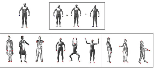
98
spherical harmonics to describe an object by a set of spherical basis functions
representing the shape histogram in a rotation-invariant manner. These
ap-100
proaches use global features to characterize the overall shape and provide a
101
coarse description, that is insufficient to distinguish similarity in 3D video
102
sequence of an object having the same global properties in the time. A
com-103
parison of these shape descriptors combined with self-similarities is made by
104
Huang et al. [12].
105
Other works on the 3D shape similarity can be found in the literature,
106
where surface-based descriptors are often used with a step of features
detec-107
tion. The advantage of these features is that their detection is invariant to
108
pose change. The extremities can be considered as the one among the most
109
important features for the 3D objects. They can be used for extracting a
110
topology description of the object like Reeb-graph descriptor [13] or closed
111
surface-based curves [14, 15, 16]. The extraction and the matching of these
112
features have been widely investigated using different scalar functions from
113
geodesic distances to heat-kernel [17, 18, 19]. Tabia et al. [14] propose to
114
extract arbitrarily closed curves amounting from feature points and use a
115
geodesic distance between curves for 3D object classification. Elkhoury et al.
116
[15] extract the same closed curves but they use heat-kernel distance in the
117
3D object retrieval process.
118
2.2. Temporal descriptors
119
Since significant progress in multiple view reconstruction techniques has
120
been made, 3D video sequences of human motion are more and more
avail-121
able. However, the need for handling and processing such data led to several
122
approaches using temporal shape representation and matching.
123
Huang et al. [12] extend the use of static descriptors to temporal ones for
frame retrieval, in a 3D human video, using time filtering and shape flows
125
obtained via invariant-rotation shape histograms. Such approaches give a
126
good shape descriptor but usually do not capture any geometrical
informa-127
tion about the 3D human body pose and joint positions/orientations. This
128
prevents using them in certain applications that require accurate estimation
129
of the pose (and the joints in some cases) of the body parts. The temporal
130
similarity in 3D video is addressed also in the case of skeletal motion and is
131
evaluated from difference in joint angle or position together with velocity and
132
acceleration [20]. Huang et al. [21] demonstrate that skeleton-based
Reeb-133
Graph descriptor has a good performance in the task of finding similar poses
134
of the same person in 3D video. Shape similarity is also used for solving the
135
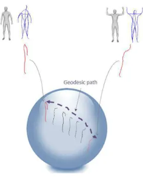
problem of video retrieval by matching frames and comparing correspondent
136
ones using a specified metric. In Yamasaki et al., [22] the modified shape
dis-137
tribution histogram is employed as feature representation of 3D models. The
138
similar motion retrieval is realized by Dynamic Programming matching
us-139
ing the feature vectors and Euclidean distance. The Dynamic Time Warping
140
algorithm (DTW), based on Dynamic Programming and some restrictions,
141
was also widely used to resolve the problem of temporal alignment. Given
142
two time series with different size, DTW finds an optimal match measuring
143
the similarity between these sequences which may vary in time or speed.
144
Thereby, by a frame descriptor and the temporal alignment using DTW,
145
many authors succeed to perform action recognition or sequence matching
146
for indexing [23, 24, 25].
147
Recently, Tung et al. [13] propose a topology dictionary for video
un-148
derstanding and summarizing. Using the Multi-resolution Reeb Graph as
a relevant descriptor for the shape in video stream for clustering. In this
150
approach, they perform a clustering of the video frames into pose clusters
151
and then they represent the whole sequence with a Markov motion graph in
152
order to model the topology change states.
153
154
From the above review, we can identify certain issues in order to consider in
155
our approach. Most of these works have attempted to use global description
156
of the model ignoring the local details. The similarity metric is usually
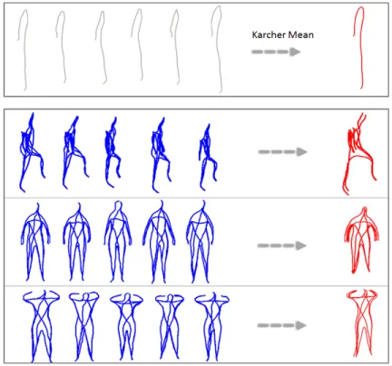
cal-157
culated directly on descriptors whereas the notion of motion is incorporated
158
by time convolution of the distance metric itself computed from static poses.
159
The video sequence is considered as a succession of frames in time and not a
160
succession of elementary motions (or gestures).
161
On one hand, the extremities feature points used in many state-of-the-art
162
algorithms can be considered as an important compact semantic
represen-163
tation of human posture. On the other hand, the shape analysis of curves
164
extracted from human body mesh allows representing the shape variations.
165
Choosing some representative curves of the body surface may provide an
166
efficient and a compact representation of human shape.
167
Our approach has several benefits: (1) the EHC descriptor can be
con-168
sidered as a surface skeletal based representation, which allows to describe
169
surface deformations of the human posture. As it is composed by a
collec-170
tion of local extremal open 3D curves, a body part representation can be
171
performed; (2) the motion analysis is incorporated in two ways, firstly by
172
time convolution of the distance metric vectors for pose retrieval in video
173
sequence, and secondly by employing motion segmentation and the notion of
clips; (3) the video segmentation allows the localization of transition states in
175
the video, in order to analyze the local dynamic of the motion, representing
176
an atomic action or gesture; and (4) an original idea is proposed to represent
177
a clip as a trajectory composed of a collection of successive frames viewed
178
as points in shape space. Finally, the video segmentation and clustering are
179
exploited in content-based summarization and motion retrieval.
180
3. Extremal Curves
181
We aim to represent a body shape as a skeleton based shape
representa-182
tion. This skeleton will be extracted on the surface of the mesh by connecting
183
features located on the extremities of the body. The main idea behind the use
184
of this representation is to analyze pose variation with elastic deformation of
185
the body, using representative curves on the surface.
186
3.1. Feature point detection
187
Feature points refer to the points of the surface located at the extremity of
188
its prominent components. They are useful in many applications, including
189
deformation transfer, mesh retrieval, texture mapping and segmentation. In
190
our approach, feature points are used to represent a new pose descriptor
191
based on curves connecting each two extremities. Several approaches have
192
been proposed in the literature to extract feature points; Mortara et al. [26]
193
select as features points the vertices where Gaussian curvature exceeds a given
194
threshold. Unfortunately, this method can miss feature points because of the
195
threshold parameter and cannot resolve extraction on constant curvature
196
areas. Katz et al. [27] develop an algorithm based on multidimensional
197
scaling, in quadratic execution complexity. Another approach more robust,
is proposed by Tierny et al. [28] to detect extremal points, based on geodesic
199
distance evaluation. This approach is used successfully to detect the body
200
extremities, since it is stable and invariant to geometrical transformations
201
and model pose. The extraction process can be summarized as the following:
202
Let v1 and v2 be the most geodesic distant vertices on a connected
tri-203
angulated surface S of a human body. These two vertices are the farthest
204
on S, and can be computed using Tree Diameter algorithm (Lazarus et al.
205
[29]). Now, let f1 and f2 be two scalar functions defined on each vertex v of
206
the surface S as follows:
207
f1(v) = g(v, v1) \ f2(v) = g(v, v2) (1)
where g(x, y) is the geodesic distance between points x and y on the
208
surface. Let E1 and E2 be respectively the sets of extrema vertices (minima
209
and maxima) of f1 and f2 on S (calculated in a predefined neighbourhood).
210
We define the set of feature points of the surface of human body S as the
211
intersection of E1 and E2. Concretely, we perform a crossed analysis in order
212
to purge non-isolated extrema, as illustrated in Figure 2 (top). The f1 local
213
extrema are displayed in blue color, f2 local extrema are displayed in red
214
color and feature points resulting from their intersection are displayed in
215
mallow color. Figure 2 (bottom) shows different persons from three different
216
datasets where feature extraction is stable despite change in shape, pose and
217
clothing for each actor.
218
3.2. Body curve extraction
219
Let M be a body surface and E = {e1, e2, e3, e4, e5} a set of feature points
220
on the body representing the output of the extraction process. Let β denotes
Figure 2: Extremity points of the 3D human body. (top) extracting process, (bottom) different human body subjects in different poses.
the open curve on M which joints two feature points of M {ei, ej}. To
ob-222
tain β, we seek for geodesic path Pij, whose length is shortest while passing
223
through the surface of the mesh, between ei and ej. We repeat this step to
224
extract extremal curves from the body surface ten times so that we do all
225
possible paths between elements of E. As illustrated in the top of Figure 3,
226
the body posture is approximated by using these extremal curves M ∼S βij,
227
and we can categorize these curves into 5 categories (Figure 3 bottom):
228
• Curves connecting hand and foot on the same side: for controlling the
229
movement of the left/right half of the body.
230
• Curves between hands and between feet: for controlling the movement
231
of the upper/lower body.
232
• Curves connecting crossed hand and foot: for controlling the movement
of the crossed limbs.
234
• Curves between head and feet: for controlling the movement of right/left
235
foot.
236
• Curves between head and hands: for controlling the movement of
237
right/left hands.
238
Figure 3: Body representation as a collection of extremal curves.
Note that modeling objects with curves is recently carried out for several
239
applications; Abdelkader et al. [30] use closed curves extracted from human
240
silhouettes to characterize human poses in 2D videos for action recognition.
241
Drira et al. [31] use open curves extracted from nose tip and face surface as
242
a surface parametrization for 3D face recognition.
243
In our approach, we have chosen to represent the body pose by a
col-244
lection of curves for two reasons. Firstly, these curves connect limbs and
give obviously a good representation of the body shape and pose, using a
246
reduced representation of the mesh surface. Secondly, this representation
247
allows studying the shape variation using Riemannian geometry by
project-248
ing these curves in the shape space of curves and using its elastic metric
249
introduced by Joshi et al. [32].
250
4. Pose modeling in shape space
251
In order to compare the similarity between two human body postures,
252
we must quantify the change of shape between correspondent curves. To do
253
this, the metric used to compare shape of curves can be computed inside an
254
open curve shape space.
255
In the last few years, many approaches have been developed to analyze
256
shapes of 2-D curves. We can cite approaches based on Fourier descriptors,
257
moments or the median axis. More recent works in this area consider a formal
258
definition of shape spaces as a Riemannian manifold of infinite dimension
259
on which they can use the classic tools for statistical analysis. The recent
260
results of Michor et al. [33], Klassen et al. [34] and Yezzi et al. [35] show
261
the efficiency of this approach for 2-D curves. Joshi et al. [32] have recently
262
proposed a generalization of this work to the case of curves defined in Rn.
263
We adopt this work to our problem since our 3-D curves are defined in R3.
264
4.1. Elastic distance
265
While human body is an elastic shape, its surface can be simply affected
266
by a stretch (raising hand) or a bind (squatting). In order to analyze human
267
curves independently to this elasticity, an elastic metric is needed within a
268
shape space framework.
Let β : I → R3, for I = [0, 1], represents an extremal curve obtained as
de-270
scribed above. To analyze its shape, we shall represent it mathematically
us-271
ing a square-root velocity function (SRVF), denoted by q(t)= ˙. β(t)/ q
k ˙β(t)k.
272
q(t) is a special function introduced by Joshi et al.[32] that captures the shape
273
of β and is particularly convenient for shape analysis.
274
The set of all unit-length curves in R3 is given by C = {q : I → R3|kqk =
275
1} ⊂ L2(I, R3), where using L2-metric on its tangent spaces, C becomes a
276
Riemannian manifold.
277
Proposition 4.1. Having two open curves represented by their SRVF, q1
278
and q2, the shortest geodesic between them in the shape space of open curves
279
is given by: α(τ ) = sin(θ)1 (sin((1 − τ )θ)q1+ sin(θτ )q2∗) ,
280
and the geodesic distance is given by: ds(q1, q2)= cos. −1(hq1, q2∗i) .
281
where q∗
2 is the optimal element associated with the optimal rotation O ∗
282
and re-parametrization γ∗
of the second curve.
283
This defined distance allows comparing shape curves regardless of
iso-284
metric and elastic deformation. In Figure 4, a geodesic path between each
285
corresponding two extremal curves, taken from two human bodies doing
dif-286
ferent poses, is computed in shape space.
287
For the left model, the person’s arm is down and for the right model it
288
is raised. The geodesic path between each two curves is shown in the shape
289
space. This evolution looks very natural under the elastic matching.
290
4.2. Static shape similarity
291
The elastic metric applied on extremal curve-based descriptors can be
292
used to define a similarity measure. Given two 3D meshes x, y and their
Figure 4: Geodesic path between two extremal human curves of neutral pose with raised hands.
descriptors x′ = {qx 1, qx2, qx3, ..., qNx} and y ′ = {qy1, q2y, q3y, ..., qNy}, the mesh-to-294
mesh similarity can be represented by the curve pairwise distances and can
295 be defined as follows: 296 s(x, y) = d(x′ , y′ ) , (2) 297 d(x′ , y′ ) = PN i=1d(β x i, β y i) N = PN i=1ds(qxi, q y i) N . (3)
where N is the number of curves used to describe the mesh. The mean of
298
curve distances between two descriptors captures the similarity between their
299
mesh poses. In case of shape change in even one curve, the global distance
300
is affected and it increases indicating that the poses are different. In order
301
to have a global distance, an arithmetic distance can be computed in order
302
to compare human poses.
4.3. Average poses
304
The use of EHC descriptor to represent the human pose by a collection
305
of 3D open curves allows analyzing the human shape using the geometrical
306
framework. It also allows computing some related statistics like ”average”
307
of several extremal human curves. Such an average, called Karcher Mean, is
308
introduced by Srivastava et al. [36]. It can be computed between different
309
poses to represent the intermediate pose, or between similar poses done by
310
several actors to represent a template for similar poses.
311
We are interested in defining a notion of ”mean” for a given set of human
312
postures in the same cluster of poses for the goal of fast pose retrieval.
313
To compute the average of EHC representation, we need only to know
314
how to compute an average for one extremal human curve. The Riemannian
315
structure defined on the shape space S enables us to perform such statistical
316
analysis for computing average and variance for each 3D open curve on body
317
surface. The intrinsic average or the Karcher Mean utilizes the intrinsic
318
geometry of the manifold to define and compute a mean on that manifold.
319
In order to calculate the Karcher Mean of extremal human curves {qα
1, ..., qαn}
320
in S, we define the variance function as:
321 V : S → R, V(µ) = n X i=1 dS(qαi, qαj)2 (4)
The Karcher Mean is then defined by:
322
qα = arg min
µ∈S V(µ) (5)
The gradient of V is used in the tangent space Tµ(S) to iteratively update
323
the current mean µ. qα is an element of S that has the smallest geodesic
path length from all given extremal human curves for the index α.
325
An example of using the Karcher Mean to compute average curve for 6
326
extremal human curves connecting hand and foot from the same side is shown
327
in the top of Figure 5, and several examples of using the Karcher mean to
328
compute average EHC representation are shown in the bottom of this figure.
329
Figure 5: Example of Karcher Mean computation. (top) Mean curve for six extremal human curves: curve connecting hand and foot from the same side. (bottom) Example of average poses computed using Karcher mean.
5. Motion segmentation and matching
330
Based on our EHC representation of the shape model, it is possible to
331
compare two video sequences by matching all pairwise correspondent
ex-332
tremal curves inside their frames, using the geodesic distance in the shape
333
space. However, a sequence of human action can be composed of several
334
distinct actions, and each one can be repeated several times. Therefore, the
335
motion segmentation can play an important role in the dynamic matching
336
by dividing the whole 3D video data into small, meaningful and manageable
337
elementary actions called clips. EHC descriptor will be employed to segment
338
continuous sequences into clips.
339
5.1. Motion segmentation
340
Video segmentation has been studied for various applications, such as
341
gesture recognition, motion synthesis and indexing, browsing and retrieval.
342
A vast amount of works in video segmentation has been performed for 2D
343
video [37], where usually the object segmentation is firstly performed before
344
the movement analysis. In Rui et al. [38], an optical flow of moving objects
345
is used and motion discontinuities in trajectories of basis coefficient over time
346
are detected. However, in Wang et al. [39], break points were considered as
347
local minima in motion and local maxima in direction change.
348
Motion segmentation is strongly applied in several algorithms using 3D
349
motion capture feature points trackable within the whole sequence, to
seg-350
ment the video. Detected local minima in motion (Shiratori et al. [40]) or
351
extrema (Kahol et al. [41]) are used in motion segmentation for kinematic
352
parameters.
Most of works on the 3D video segmentation use the motion capture
354
data, and very few of them were applied to dynamic 3D mesh. One of them
355
is presented by Xu et al. [42], where a histogram of distance among vertexes
356
on 3D mesh is generated to perform the segmentation through thresholding
357
step defined empirically. In Yamasaki et al. [43], the motion segmentation is
358
automatically conducted by analyzing the degree of motion using modified
359
shape distribution for mainly japanese dances. These sequences of motion
360
are paused for a moment and then they are consider as segmentation points.
361
Huang et al. [44] propose an automatic key-frame extraction method for
362
3D video summarization. To do so, they compute the self similarity matrix
363
using volume-sampling spherical Shape Histogram descriptor. Then, they
364
construct a graph based on this self similarity matrix and define a set of key
365
frames as the shortest path of this graph.
366
In our work, we propose an approach fully automatic to segment a 3D
367
video efficiently without making neither thresholding step nor assumption on
368
the motion’s nature. In motion segmentation, the purpose is to split
automat-369
ically the continuous sequence into segments which exhibit basic movements,
370
called clips. As we need to extract meaningful clips, the segmentation is
371
overly fine and can be considered as finding the alphabet of motion. For a
372
meaningful segmentation, motion speed is an important factor. In fact, when
373
human changes motion type or direction, the motion speed becomes small
374
and this results in dips in velocity. We exploit this latter by finding the local
375
minima for the change in type of motion and local maxima for the change
376
in direction. The extrema detected on velocity curve should be selected as
377
segment points (see Figure 6). We show frames detected as maxima (the
tor changes the foot’s direction) on the top of the plot, and frames detected
379
as minima (the actor raise the other foot) on the bottom. In this work, we
380
consider only the change in type of motion as a meaningful clip. Thus, clips
381
with slight variations and a small number of frames are avoided.
382
Figure 6: Segmentation of a 3D sequence into motion clips. Feature vector and detected frames as local extrema are presented at the top of the figure and detected frames as minima are at the bottom.
Note that optimum local minimum, that detect precise break points where
383
the motion changes, is selected in a predefined neighbourhood. For this
384
raison, we fix a size of window to test the efficiency of the local minimum in
this condition. To calculate the speed variation, distance between each two
386
successive EHC in the sequence is computed. The variations of the sequence
387
are represented in vector of speed and a further smoothing filter is applied
388
to obtain the final degree of motion vector.
389
5.2. Clip matching
390
To seek for similar clips, we need to encode gestures in a specific
repre-391
sentation that we can compare regardless to certain variations. In fact, two
392
motions are considered similar even if there are changes in the shape of the
393
actor and the speed of the action execution. This problem is similar to
time-394
series retrieval where a distance metric is used to look for, in a database, the
395
sequences whose distance to the query is below a threshold value. Each clip
396
is represented as a temporal sequence of human poses, characterized by EHC
397
representation associated to shape model. Then, extremal curves are tracked
398
in each sequence to characterize a trajectory of each curve in the shape space
399
as illustrated in Figure 7 (top). Finally, the trajectories of each curve are
400
matched and a similarity score is obtained. However, due to the variations
401
in execution rates of the same clip, two trajectories do not necessarily have
402
the same length. Therefore, a temporal alignment of these trajectories is
403
crucial before computing the global similarity measure, as shown in Figure 7
404
(bottom).
405
In order to solve the temporal variation problem, we use DTW algorithm
406
(Giorgino et al. [45]). This algorithm is used to find optimal non-linear
407
warping function to match a given time-series with another one, while
ad-408
hering to certain restrictions such as the monotonicity of the warping in the
409
time domain. The optimization process is usually performed using dynamic
Figure 7: Graphical illustration of a sequence of shapes obtained during a walking action (top). Alignment process between trajectories of same curve index using DTW (bottom).
programming approaches given a measure of similarity between the features
411
of the two sequences at different time instants. The global accumulated costs
412
along the path define a global distance between the query clip and the motion
413
segments found in the database. Since DTW can operate with any measure
414
of similarity between different temporal features, we adapt it to features
415
that reside on Riemannian manifolds. Hence, we use the geodesic distance
416
between different shape points ds(qi, qj) as a distance function between the
417
shape features at different time instants.
In practice, the first step is to follow independently curve variation in
419
time resulting on N trajectories in the shape space. In fact, each frame
420
in the 3D video sequence can be represented by a predetermined number
421
(N) of extremal curves, splitting the sequence into N parts, where each one
422
represents the trajectory of an open curve in the shape space. Then, DTW
423
will be applied in the feature space for each tracked curve index. The distance
424
between two clips is then the average distance given by each comparison
425
between corresponding trajectories.
426
5.3. Average clip
427
Based on the two algorithms, Karcher Mean and DTW, we can extend
428
the notion of “mean” of a set of human poses to the “mean” of trajectories
429
of poses in order to compute an ”average” of several clips.
430
Let N be the number of clips represented by N trajectories T1, T2· · · TN.
431
For a specific human curve index, we look for the mean trajectory that has
432
the minimum distance to the all N trajectories.As shown in Algorithm 1,
433
the mean trajectory is given by computing the non-linear warping functions
434
and setting iteratively the template as the Karcher Mean of the N warped
435
trajectories represented in the Riemannian shape space.
436
6. Video summarization and retrieval
437
In order to represent compactly a video sequence, we need to know how
438
to exploit the redundancy of information over time. However, when this
in-439
formation should be extracted from motion and not from frames separately,
440
the challenge is then about complex matching processes required to find
ge-441
ometric relations between consecutive data stream elements. We therefore
Algorithm 1 Computing trajectory template Require: N trajectories from N clips T1, T2· · · TN
Initialization: chose randomly one of the N input trajectories as an initial guess of the mean trajectory Tmean
repeat
fori=1 : N do
find optimal path p∗ using DTW to warp Ti to Tmean
end for
Update Tmean as the Karcher Mean of all N warped trajectories
untilConvergence
propose to use EHC to represent a pose and a trajectory as key descriptors
443
characterizing geometric data stream. Based on EHC representation, we
de-444
velop several processing modules as clustering, summarization and retrieval.
445
6.1. Data clustering
446
Let V denotes a video stream of human sequence containing elements
447
{ei}i=1...k, where e can be a frame or a clip. To cluster V , the data set is
448
recursively split into subsets Ctand Rtas described in the following recursive
449
algorithm:
450
Algorithm 2 Data clustering Require: V{ei}i=1...k; Ensure: C0= ∅ ; R0= {e1, . . . , ek}; if (Rt6= ∅)&&(t <= k) then Ct= {f ∈ Rt−1: dist(et, f) < T h}; Rt= Rt−1\ Ct; end if
The result of clustering is contained in Ct=1..k where Ct is a subset of V
representing a cluster containing similar elements to et. For each iteration of
452
clustering steps, from t = 1 · · · K, the closest matches to etare retrieved and
453
indexed with the same cluster reference as et. Any visited element etalready
454
assigned to a cluster in C during iteration step is considered as already
clas-455
sified and is not processed subsequently. We regroup not empty sub sets Ct
456
in l clusters {c1, ..., cl} (with l 6 k). Similarities between elements of V are
457
evaluated using a similarity distance dist allowing to compare the elements
458
of V . The threshold T h is defined experimentally .
459
If we consider the video V as a long stream of 3D meshes, the clusters that
460
should be obtained must gather models with similar poses. In this case, the
461
EHC feature vector is used as an abstraction for every mesh and the similarity
462
distance is the elastic metric computed between each pair of human poses.
463
Motion can be incorporated in this similarity by applying a simple time
464
filter on static similarity measure with a window size chosen experimentally
465
[46]. The use of temporal filter integrates consecutive frames in a fixed time
466
window, thus allowing the detection of individual poses while taking into
467
account smooth transitions. Note that the pose invariance property of the
468
EHC allows us to compare poses (and motions) of subjects regardless of
469
translation, rotation and scaling .
470
The video V can also be considered as a stream of clips resulting from
471
the video segmentation approach and clusters here gathers clips with similar
472
repeated atomic actions. In this case: (1) the feature vector used as
abstrac-473
tion for each clip is a trajectory on shape space of extremal human curves;
474
and (2) the similarity distance, used to compare clips, is based on the DTW
475
algorithm.
6.2. Content-based summarization
477
Our approach for video summarization is based on three steps: First, the
478
whole video is segmented and clustered into several clusters of clips. Second,
479
only the most significant clip (the nearest one to all cluster elements) of each
480
cluster is kept. Third, we construct a subsequence, from the starting video,
481
where this representative clips of each cluster are concatenated. Finally,
482
This new subsequence, is clustered into clusters of poses, and only most
483
representative poses are kept to describe the dataset.
484
This summarization allows a reduction of dimension for the original dataset
485
where we can display only main clips if we stop on third step, or to display
486
key frames if we continue summarization process until pose clustering.
487
6.3. Pose and motion Retrieval
488
As in a classical retrieval procedure, in response to a given query, an
489
ordered list of responses that the algorithm found nearest to the query is
490
given. Then to evaluate the algorithm, this ranked list is analyzed. Whatever
491
the given query, pose or clip, the crucial point in the retrieval system is the
492
notion of ”similarity” employed to compare different objects.
493
For content-based pose retrieval, thanks to the static shape similarity, we
494
are able to compare human poses using their extremal human curve
descrip-495
tors and decide if two poses are similar or not. In this scenario, the query
496
consists of a 3D human shape model in a given pose and the response is 3D
497
human bodies more similar in pose to the query. We advocate the usage of
498
the EHC to represent the 3D human shape model in a given pose and then
499
comparison between each pair of models using the elastic metric defined in
the Proposition 4.1. This system can find a number of utilities like
pose-501
based searching and facilitate retrieval of efficient information as subjects in
502
same poses in the database of 3D models scanned in different poses [47, 48].
503
Note also that identifying frames with similar shape and pose can be used
504
potentially for concatenative human motion synthesis. Concatenate existing
505
3D video sequences allows the construction of a novel character animation. A
506
good descriptor that much correctly correspondent frames allows the
synthe-507
sis of videos with smooth transitions and finding best frames to summarize
508
the video. However, extension of static shape descriptor to include
tem-509
poral motion information is required to remove the ambiguities inherent in
510
static shape descriptor for comparing 3D video sequences of similar shape.
511
Therefore, the static shape descriptor can be extended to the time domain
512
by applying a simple time filter with a window size like 2Nt+ 1. This time
513
filter is a way of incorporating motion in the similarity measure, as so-called
514
temporal similarity, also used by Huang et al. [12]. The temporal similarity
515
is presented in the following Equation:
516 st ij = 1 2Nt+ 1 Nt X k=−Nt s(i + k, j + j) (6)
where s is the frame-to-frame similarity matrix and Nt is a time filter with
517
window size 2Nt+ 1.
518
For content-based motion retrieval, we advocate the usage of the EHC
519
representation, where a query consists of a trajectories representing a clip on
520
the shape space. As response to this specific query, our approach looks in the
521
sequence for most similar trajectories and returns an ordered list of similar
522
ones using the process of motion clip explained in section 5.2.
7. Experimental results
524
To show the practical relevance of our method, we perform an
experimen-525
tal evaluation on several databases (summarized in Table 1) and compare it
526
to the most efficient descriptors of the state-of-the-art methods. We first
eval-527
uate our descriptor for shape similarity application over public static shape
528
database [48] and evaluate the results against Spherical Harmonic descriptor
529
[11]. Secondly, we measure the efficiency of our descriptor to capture the
530
shape similarity in 3D video sequences of different actors and motions from
531
other public 3D synthetic [12] and real [49, 50] video databases. We evaluate
532
this later against Temporal Shape Histogram [12], Multi-resolution
Reeb-533
graph [21] and other classic shape descriptors, using provided Ground Truth.
534
Motion segmentation into clips and clip matching performance are tested on
535
several video sequences of different people doing different motions. Finally,
536
we evaluate our clustering and summarization approach for pose/clip-based
537
video retrieval.
538
7.1. Feature matching
539
The extraction and comparison of our curves requires the identification of
540
feature end-points as head, right/left hand and right/left foot, which is not
541
affordable in practice. This requirement is important to perform the curve
542
matching separately between models. In order to overcome this problem,
543
our method is based on two benefits from the morphology of the human
544
body. First, we deduce that geodesic path connecting each one of the hand
545
end-points and the head end-point is shortest among all possible geodesics
546
between the five end-points. Second, the geodesic path connecting right hand
Dataset Motions/Poses Number of frames Dataset (1) [48]:
144 subjects (59 men/55 women)
18 static poses (1 neutral done by all subjects and 17 other dif-ferent poses)
⊘
Dataset (2) [12]: 14 people (10 men and 4 women)
28 motions: sneak, walk (slow, fast, turn left/right, circle left/right, cool, cowboy, elderly, tired, ma-cho, march, mickey, sexy,dainty), run (slow, fast,turn right/left, cir-cle left/right), sprint, vogue, faint, rockn’roll, shoot.
392 seq, 39200f (100f per seq.)
Dataset (3) [49]: 3 people (2 men and 1 woman)
6 motions: 2×cran, 2×marche, 2×squat, 1×handstand, 1×samba, 1×swing.
1582f (on average 226 ± 48 per seq.)
Dataset (4) [50]: Roxanne
Game character motion: walk 32 f
Table 1: Summarization of data used for all experimental tests.
to left foot end-points or left hand to right foot end-points is the longest. The
548
first observation allows to identify precisely the end-point corresponding to
549
the head, the two end-points connected to this later corresponding to the
550
hands without distinguishing between right and left. The second one allows
551
the identification of the couple of hand/foot as corresponding to same side of
552
the body without distinguishing between right and left. A prior knowledge
553
on the direction of the posture of the human body for static pose and in the
554
starting frame for video sequence has allowed to distinguish between left and
right. Once the end-points are correctly detected from the starting frame
556
in the video sequence, a simple algorithm of end-point tracking over time is
557
performed.
558
7.2. Static shape similarity
559
The protocol and the dataset used to validate the experiments are firstly
560
presented and then, the results following this protocol are analyzed and
com-561
pared to those obtained by other approaches.
562
7.2.1. Evaluation methodology
563
To assess the performance of the EHC for static shape similarity,
sev-564
eral experiments were performed on a statistical shape database [48]. This
565
database, summarized in Table 1 (1st row), is challenging for human body
566
shape and pose retrieval as it is realistic shape database captured with a
567
3D laser scanner. It contains more than hundred subjects doing more than
568
thirty different poses. We perform our descriptor on a subset of 338 shape
569
models obtained from 144 subjects 59 male and 55 female aged between 17
570
and 61 years. There are 18 consistent poses (p0, p1, p2, p3, p4, p5, p6, p7,
571
p8, p9, p10, p11, p12, p13, p16, p28, p29, p32). Some poses are illustrated
572
in Figure 8. Each pose represents a class where at least 4 different subjects
573
do the same pose.
574
For evaluation, we use Recall/Precision plot in addition to the three
575
statistics which indicate the percentage of the top K matches that belong to
576
the same pose class as the query pose:
577
• The nearest neighbor statistic (NN): it provides an indication to how
578
well a nearest neighbor classifier would perform (here K = 1).
Figure 8: Example of body poses in the static human dataset [48].
• The first tier statistic (FT): it indicates the recall for the smallest K
580
that could possibly include 100% of the models in the query class.
581
• The second tier statistic (ST): it provides the same type of result, but
582
it is a little less stringent (i.e., K is twice as big).
583
• E-Measures: it is a composite measure of precision and recall for a fixed
584
number of retrieved results.
585
We note here that these statistics will be used for static and video retrieval
586
evaluations.
587
7.2.2. Curve selection
588
From five feature endpoints, we have extracted ten extremal curves
rep-589
resenting the human body shape model. According to the human poses,
590
extremal curves exhibit different performance and some curves are more
effi-591
cient to capture the shape similarity between two poses. Our shape descriptor
can be seen as a concatenation of ten curve representations and the similarity
593
between two shape models doing two different poses, is represented by a
vec-594
tor of ten elastic distance values. Before all tests, we analyze the performance
595
of all possible combinations of curves on the shape similarity measurements.
596
A Sequential Forward Selection method, applied on elastic distance values
597
and coupled with ST statistic, has been used to select the best combination
598
of curves among all possible ones (1013 combinations according to Eq. 7):
599 n X k=2 Ck n = n X k=2 n! k!(n − k)! (7)
where n is equal to 10 and it represent the number of curves.
600
Experiment of pose-based retrieval on the dataset [48] shows that the best
601
combination is obtained by the five curves: right hand to right foot, left hand
602
to left foot, left hand to right hand, left foot to right foot, and head to the
603
right foot (Figure 9).
604
The selected five curves seem to be the most stable ones and they are
605
sufficient to represent at best the body like a skeleton on the surface.
There-606
fore, the elimination of five curves allows to eliminate the ambiguity due to
607
the redundancy of some curves on the body parts.
608
7.2.3. Result analysis
609
The self similarity matrix obtained from the mean elastic distance of the
610
five selected curves is shown in the Figure 10.
611
This matrix demonstrates that similar poses have a small distance (cold
612
color) and that this distance increases with the degree of the change
be-613
tween poses (hot color). This allows pose classification or pose retrieval by
Figure 9: Second-Tier statistic for all combinations of curves. The best combination is obtained by 5 curves (green) and the worst combination is obtained by 2 curves (red).
comparing models using their extremal curve representation and the elastic
615
metric.
616
From a quantitative point of view, we present the Recall/Precision plot
617
obtained by EHC compared to the popular Spherical Harmonic (SH)
descrip-618
tor with optimal parameter setting (Ns= 32 and Nb = 16) [8]. This plot and
619
accuracy rates (NN, FT and ST) reported in Table 2 show that our approach
620
provides better retrieval precision. EHC using only the five selected curves
621
outperforms SH and EHC using the 10 curves to retrieve models with the
622
same pose.
623
Note finally that the accuracies of retrieval ranks for some poses are
rela-624
tively low. Such ambiguities can be noticed in the case of comparison between
625
neutral pose and a pose where subjects just twist their body to the left, or
Figure 10: Confusion similarity matrix. The matrix contains pose dissimi-larity computation between models of a 3D humans in different poses. More the color is cold more the two poses are similar.
Approach NN(%) FT(%) ST(%) E-Measure(%)
SH 71.0 57.9 75.5 41.3
EHC 10 curves 80.3 75.5 85.2 42.5 EHC 5 curves 84.8 77.2 89.1 43.0
Table 2: Retrieval statistics for pose based retrieval experiment
twist their torso to look around.
Figure 11: Precision-recall plot for pose-based retrieval.
7.3. Temporal shape similarity for 3D video sequences
628
We firstly present the protocol and the dataset used in these experiments
629
and then, the results following this protocol are analyzed and compared to
630
the most relevant state-of-the-art approaches.
631
7.3.1. Evaluation methodology
632
The recognition performance of the temporal shape descriptor is evaluated
633
using a ground-truth dataset from a synthetic 3D video sequences proposed
634
by Huang et al. [12] and a real captured 3D video sequences of people [49].
635
As described in Table 1 (2nd raw), the synthetic data is obtained by 14 people
636
(10 men and 4 women) performing 28 motions. Each sequence is composed
637
of 100 frames and the whole dataset contains a total of 39200 frames.
638
Given the known correspondences, a temporal ground-truth similarity is
639
computed between each two surfaces. The known correspondence is only
used to compute this ground truth similarity. Having two Mesh X and Y
641
with N vertices xi ∈ X and yi ∈ Y , a temporal-ground truth CT is computed
642
by combining a shape similarity Cp and a temporal similarity Cv as follows:
643 CT(X, Y ) = (1 − α)Cp(xi, yj) + αCv(xi, yj) Cp(X, Y ) = N1 PN k=1d(xi, yj) Cv(X, Y ) = N1PNk=1d( ˙xi, ˙yj) (8)
where d is an Euclidean distance, ˙xi and ˙yj are the derivation of x and
644
y between next and current frame. the parameter α is used to balance the
645
equation and it is set to 0.5 . In order to identify frames as similar or
646
dissimilar, the temporal ground truth similarity matrix is binarized using a
647
threshold set to 0.3 similarly to Huang et al. [12].
648
Finally, recognition performance is evaluated using the
Receiver-Operator-649
Characteristic (ROC) curves, created by plotting the fraction of true-positive
650
rate (TPR) against the fraction of false-positive rate (FPR), at various
651
threshold settings. The true and false dissimilarity compare the predicted
652
similarity between two frames, against the ground-truth similarity.
653
An example of self-similarity matrix computed using temporal
ground-654
truth descriptor, static and temporal descriptors are shown in Figure 12.
655
This figure illustrates also the effect of time filtering with increasing temporal
656
window size for EHC descriptors on a periodic walking motion.
657
7.3.2. Result analysis
658
A comparison is made between our Temporal Extremal Human Curve
659
(TEHC) and several descriptors from the state-of-the-art: Shape
Distribu-660
tion (SD) , Spin Image (SI) , Spherical Harmonics Representation (SHR),
Figure 12: Similarity measure for ”Fast Walk” motion in a straight line com-pared with itself. Coldest colors indicate most similar frames. 1st matrix:
temporal Ground-Truth (TGT). 2nd, 3rd and 4th matrix: self-similarity
ma-trix computed with Temporal EHC with window size 3, 5 and 7 respectively.
two Shape-flow descriptors, the global / local frame alignment Shape
His-662
tograms (SHvrG / SHvrS) (Huang et al. [12]) and Reeb-Graph as skeleton
663
based shape descriptors (aMRG) (Tung et al. [51]). Note that a spectral
664
representation was also evaluated by Huang et al. [21] which is the
Multi-665
Dimentional Scaling (MDS). Huang et al. [12] evaluated the performances
666
of all these descriptors for the purpose of shape similarity.
667
The effectiveness of our descriptor have been evaluated by varying temporal
668
window and comparing it to the most relevant state-of-the-art descriptors
669
[12] as shown in the plot of ROC curves in Figure 13.
670
Several observations can be made on the obtained results: (i) Our
descrip-671
tor outperforms classic shape descriptors (SI, SHR, SD) and shows
compet-672
itive results with SHvrS and aMRG. We also notice that recognition
perfor-673
mance of EHC increases with the increase of the window size of time-filter
674
like any other descriptor. In fact, time-filter reduces the minima in the
anti-675
diagonal direction, resulting from motion in the static descriptor (Figure 13).
Figure 13: Evaluation of ROC curve for static and time-filtered descriptors on self-similarity across 14 people doing 28 motions. From right to left: ROC curves obtained by our TEHC descriptor with three different values of windows size Nt, ROC curve obtained by our EHC descriptor compared to different algorithms and ROC curves obtained with Nt= 1.
Multiframe shape-flow matching required in SHvrS allows the descriptor to
677
be more robust but the computational cost will increase by the size of
se-678
lected time window.
679
(ii) EHC descriptor by its simple representation, demonstrates a comparable
680
recognition performance to aMRG. It is efficient as the curve extraction is
681
instantaneous and robust as the curve representation is invariant to elastic
682
and geometric changes thanks to the use of the elastic metric.
683
(iii) The result analysis for each motion shows that EHC gives a smooth
684
rates that are stable and not affected by the complexity of the motion. Such
685
complex motions are rockn’roll, vogue dance, faint, shot arm (Figure 14).
686
However, this is not the case for SHvrS where performance recognition falls
687
suddenly with complex motions as illustrated in Figure 15.
688
Figure 14: Evaluation of EHC descriptor against Temporal Ground Truth (TGT) for Nt=0 and Nt=1. ROC performance for 28 motions across 14 people.
We also applied the time filtering EHC descriptor on two real captured 3D
690
video sequences of people. The first sequence is extracted from the dataset
691
[49] described in Table 1 (3rd row). The second one is extracted from real
692
data reconstructed by multiple camera video [50] and described in Table 1
693
(4th row).
694
Inter-person similarity across two people in a walking motion with an
695
example similarity curve are shown in Figure 16 (a). Our temporal similarity
696
measure identifies correctly similar frames across different people. These
697
similar frames are located in the minima of the similarity curve. In addition,
(a) Vogue (b) Faint
(c) Shot arm (d) Rockn’roll
Figure 15: Evaluation of ROC curves for complex motions with Nt=3.
despite the topology change and the reconstruction noise as shown in Figure
699
16 (b), our algorithm succeed to identify correctly the frame in the sequence
700
similar to the query.
701
7.4. Motion segmentation and retrieval
702
In this section, we evaluate temporal shape similarity descriptor. Details
703
about the computation of the ground truth descriptor are given in addition
704
to the description of the different datasets used for evaluation. The results
705
obtained by our approach, compared to those of different state-of-the-art
(a) (b)
Figure 16: Inter-person similarity measure for real sequences. Similarity matrix, curve and example frames for (a) Walk motion across two actors [49] (b)walk motion for Roxanne [50] Game Character Walk .
descriptors, are then discussed.
707
7.4.1. Evaluation methodology
708
The two datsets (2) and (3) presented in Table 1 are used in these
experi-709
ments. From the synthetic dataset [12], we have chosen 14 different motions:
710
walk (slow, fast, circle left/right, cowboy, march, mickey), run (slow, fast,
711
circle left/right), sprint, and rockn’roll. These motions are performed by two
712
actors (a woman and a man) making a total of 28 motions (2800 frames).
713
They are chosen for their interesting challenges as: (i) change in execution
rate (slow/fast motions) (ii) change in direction while moving (walking in
715
straight line, moving in circle and turning left and right) (iii) change in
716
shape (a woman and a man). We used these motion sequences for both
717
segmentation and retrieval experiment.
718
To validate the segmentation step, we segment all these 3D video
se-719
quences with the proposed approach and then compare results to manual
720
segmentation ground-truth. In the retrieval process, each query clip is
com-721
pared to all other clips obtained by the segmentation of sequences. Finally,
722
the statistics (NN, FT, ST and E-measure) are used for the evaluation.
723
7.4.2. Analysis of motion segmentation result
724
Plotting the distance between EHC representation of successive frames
725
gives a very noisy curve. The break points from this curve do not define
726
semantic clips and the extracting of minima leads to an over-segmentation of
727
the sequence (see Figure 17 (top)). To obtain more significant local minima,
728
we convolve the curve with a time-filter allowing to take into account the
729
motion variation, not only between two successive frames but also in a time
730
window. The motion degree after convolution is shown in Figure 17 (bottom).
731
Break points are more precise and delimits significant clips corresponding to
732
step change in the video sequence. In order to evaluate its efficiency, we
733
apply our segmentation method on the whole dataset (3) described in Table
734
1 (3rd raw) and then compare the results to a manual segmentation of the
735
base done carefully .
736
We performed the clip segmentation for all window size values from 1
737
to 11 over a representative set of clips extracted from the dataset (3) [49].
738
Compared to manual ground truth, the best segmentation is obtained using
a window size of 5. This value is then fixed for the rest of the tests. The
740
segmentation of the dataset(3) gives 83 segmented clips (78 correct clips and
741
5 incorrect clips). This can be explained by the fact that the 5 failing clips
742
are short. They contain about 6 frames at most and do not describe atomic
743
significant actions. Otherwise, the a total of 144 clips have been obtained by
744
the segmentation of the 14 motions taken from the dataset (2) described in
745
Table 1 (2nd raw) performed by two actors.
746
Figure 17: Speed curve smoothing.
Figure 18 shows some results of motion segmentation on a ”slow walk”
747
and a ”fast walk” motions. Although the walk speed increases, the motion
segmentation remains significant and does not change and corresponds to the
749
step change of the actor. The Rockn’roll dance motion segmentation is also
750
illustrated in Figure 18 (bottom). Thanks to the selection of local minima
751
in a precise neighborhood, only significant break points are detected.
752
Figure 18: Various motion segmentation. From right top to left bottom, motions are: slow walk, Rockn’roll dance, fast walk, vogue dance.
7.4.3. Analysis of motion retrieval result
753
The motion segmentation method, applied on 14 motion sequences from
754
the dataset (2) and performed by a man and a woman, gives a total of
755
144 clips. These clips, with an average number of frames per clip equal to
756
15, are categorized into 14 classes. The motion sequences consist mainly
757
of different styles of walking, running and some dancing sequences. Classes
758
grouped together represent different styles of walking, running and dancing
759
steps. For example, a step change in a walk may represent a class and groups


![Figure 8: Example of body poses in the static human dataset [48].](https://thumb-eu.123doks.com/thumbv2/123doknet/12429698.334432/33.918.293.621.193.413/figure-example-body-poses-static-human-dataset.webp)

