Searching for dark matter with superheated liquid detectors

Searching for dark matter with superheated liquid detectors

par Arthur Plante

Département de Physique Faculté des arts et des sciences

Thèse présentée à la Faculté des études supérieures en vue de l’obtention du grade de Philosophiæ Doctor (Ph.D.)

en physique

Mars, 2019

c

Faculté des études supérieures

Cette thèse intitulée:

Searching for dark matter with superheated liquid detectors

présentée par: Arthur Plante

a été évaluée par un jury composé des personnes suivantes: François Schiettekatte , président-rapporteur

Viktor Zacek, directeur de recherche Thomas Brunner , membre du jury

De nos jours, l’une des questions fondamentales en physique des particules est la nature de la matière sombre. Les expériences PICASSO et PICO sont deux expériences de détection directe de matière sombre qui sont situées à SNOLAB qui utilisent des chambres à bulles remplies de fréons surchauffés. La collaboration PICASSO a mis sur pied la première expérience à utiliser des chambres à bulles dans le but spécifique de détecter la matière sombre et à de plus découvert l’existence de la discrimination acoustique entre les neutrons et les particules alpha. Le dernier résultat de l’expérience PICASSO a été publié en 2017 et possède, jusqu’à ce jour, la meilleure limite sur la section efficace d’interaction entre la matière sombre et la matière baryonique qui dé-pend du spin pour des masses de WIMPs inférieure à 5 GeV/c2 avec une limite de σ_pSD = 7× 10−2pb (90% C.L). Depuis la fusion des collaborations PICASSO et PICO, l’expérience PICO détient la meilleure limite au monde pour toute autre masse de WIMP et dont la meilleure limite correspond à σ_pSD= 2.5_×10−5pb (90% C.L) pour des WIMP de 25 GeV/c2. Actuellement, la collaboration PICO est en train de construire le détecteur PICO40L dont le bruit de fond dû aux neutrons sera radicalement diminué par un fac-teur_{∼50 et qui sert de prototype pour le design et la construction du prochain détecteur,} PICO500, qui contiendra environ 500L de fréon.

Cette thèse présentera tout d’abord les aspects théoriques de la matière sombre, c’est-à-dire les preuves de son existence (Chap. 2), les particules candidates les plus probables (Chap. 3), ainsi que les spectres des énergies de reculs et le taux de comptage attendu dans un détecteur de matière sombre (Chap. 4). Ces chapitres seront suivis de la pré-sentation de la technique de détection de matière sombre avec des chambres à bulles contenant des liquides en surchauffe (Chap. 5) en plus des descriptions des détecteurs PICASSO et PICO (Chap. 6 & 7) ainsi que de l’étalonnage de ces détecteurs (Chap. 8) et de leurs résultats (Chap. 9 & 10). Par la suite, les résultats des simulations du bruit de fond de PICO40L dû aux neutrons seront présentés (Chap. 11) de même que la présenta-tion du rôle de l’expérience PICO dans le contexte de la théorie effective (Effective Field

Theory) de la matière sombre (Chap. 12). Finalement, la recherche et le développement actuel et futur de l’expérience PICO, par exemple, la description de PICO500 ainsi que la possibilité d’utiliser du C2H2F4comme liquide actif seront présentés dans le dernier

chapitre (Chap. 13).

Mots clés: Matière sombre, détecteurs à liquide surchauffées, simulation, PICO, PICASSO, WIMPs.

One of the most prominent questions in the fields of particle physics and cosmol-ogy is the nature of dark matter which comprises 85% of the total mass of the universe. The PICASSO and PICO experiments are both direct detection experiments situated at SNOLAB that use the superheated liquid or bubble chamber technique to search for dark matter. The PICASSO collaboration pioneered the use of this technique for dark mat-ter searches, and moreover, discovered an important background suppression feature: the acoustic alpha-neutron discrimination. The last PICASSO result was published in 2017 and still holds to this day the best spin-dependent cross-section limit of 7_×10−2pb (90% C.L.) for weakly interacting dark matter candidates (WIMPs) with a mass of 4 GeV/c2 [1]. Since the merger of PICASSO and COUPP into PICO, PICO holds the world best limit on WIMP cross sections with the most stringent spin-dependent limit of 2.5_×10−5pb (90% C.L) at 25 GeV/c2 set by the recent PICO60 detector result [2]. The PICO collaboration is currently building a new detector called PICO40L with a sig-nificantly improved design which will allow to substantially decrease the neutron back-ground by a factor of_{∼50, and pave the way forward for the next stage, PICO500, which} will contain approximately 500L of superheated liquid.

The present work presents first the observational and theoretical framework of dark matter searches, i.e., its proof of existence (Chap. 2), the most probable particle can-didates (Chap. 3), as well as its expected recoil spectra and count rates in typical dark matter detectors (Chap. 4). It will be followed by a description of the superheated liquid technique (Chap. 5), by the description of the PICASSO and PICO detectors (Chap. 6 & 7), of their calibrations and common backgrounds (Chap. 8). In Chap. 9 & 10, the final PICASSO result are presented together with the most recent PICO dark matter limits. A GEANT4 simulation of the PICO40L neutron background will then be described in detail (Chap. 11), along with a discussion of the physic reach of PICO within the context of the effective field theory description of dark matter (Chap. 12). Finally, this thesis concludes with the current and future research and development program of the PICO

collaboration, such as the future PICO500 detector, and the exciting possibility of using C2H2F4as an active target (Chap. 13).

RÉSUMÉ . . . iii

ABSTRACT . . . v

CONTENTS . . . vii

LIST OF TABLES . . . xii

LIST OF FIGURES . . . xv

LIST OF APPENDICES . . . .xxxv

LIST OF ABBREVIATIONS . . . .xxxvi

CHAPTER 1: INTRODUCTION . . . 1

CHAPTER 2: DARK MATTER IN THE UNIVERSE . . . 4

2.1 Lambda Cold Dark Matter model . . . 4

2.2 Observational evidences of dark matter . . . 6

2.2.1 Distribution of galaxy velocities in clusters . . . 6

2.2.2 Rotations curves of spiral galaxies . . . 7

2.2.3 Gravitational lensing . . . 8

2.2.4 Inhomogeneity of the cosmic microwave background . . . 10

2.2.5 Primordial nucleosynthesis BBN (Big Bang nucleosynthesis) . . 13

2.2.6 The WIMP miracle . . . 17

2.2.7 21 cm line . . . 18

CHAPTER 3: DARK MATTER CANDIDATES . . . 23

3.1 Baryonic dark matter . . . 23

3.2 The axions . . . 23

3.4 Hot dark matter . . . 27

3.5 Cold dark matter . . . 28

3.6 Supersymmetry . . . 28

3.7 The MSSM and the neutralino . . . 29

3.8 Asymmetric dark matter . . . 29

CHAPTER 4: DETECTION OF DARK MATTER . . . 31

4.1 The WIMP in the universe and in the Milky Way . . . 32

4.2 Direct detection . . . 34

4.3 Expected WIMP signal . . . 36

4.4 Direct detection techniques . . . 41

4.4.1 Liquid noble gas detectors . . . 41

4.4.2 Solid state detectors . . . 43

4.4.3 Superheated liquids . . . 44

4.5 Current limits . . . 44

4.6 Dark matter production . . . 47

4.7 Indirect detection . . . 49

CHAPTER 5: SUPERHEATED LIQUID DARK MATTER DETECTORS 51 5.1 Bubble chambers . . . 51 5.2 Superheated liquids . . . 55 5.2.1 Critical radius . . . 60 5.2.2 Seitz Model . . . 62 5.3 Bubble growth . . . 66 5.4 Acoustic emission . . . 70

5.5 Acoustic response to different target fluids . . . 72

CHAPTER 6: THE PICASSO EXPERIMENT . . . 77

6.1 Piezoelectric sensors . . . 80

6.2 Data taking at SNOLAB . . . 81

6.4 Data acquisition system . . . 84

CHAPTER 7: THE PICO EXPERIMENT . . . 88

7.1 PICO detector working principle . . . 88

7.1.1 RSU versus normal design . . . 89

7.1.2 Pressure vessel . . . 91

7.1.3 Pressure system . . . 91

7.1.4 Read out systems . . . 91

7.1.5 PICO detector operation . . . 92

7.1.6 Background and simulations . . . 93

7.2 Data analysis . . . 94

7.2.1 3D position reconstruction . . . 94

7.2.2 Fast pressure transducer analysis . . . 96

7.2.3 Acoustic analysis . . . 97

7.3 History of PICO detectors . . . 100

7.3.1 PICO 60 (CF3I) . . . 101

7.3.2 PICO 2L . . . 101

7.3.3 PICO60 (C3F8) . . . 103

7.3.4 PICO40L . . . 104

CHAPTER 8: CALIBRATION AND BACKGROUND OF PICO AND PI-CASSO DETECTORS . . . 106

8.1 Neutron interactions with freons . . . 107

8.2 6 MV Pelletron Tandem accelerator . . . 110

8.3 Monoenergetic neutron production . . . 111

8.4 Neutron calibration measurements . . . 115

8.4.1 PICASSO neutron calibrations . . . 115

8.5 PICO neutron calibrations . . . 118

8.5.1 The C3F8neutron beam calibrations . . . 119

8.5.2 C3F8SbBe neutron calibration . . . 120

8.6.1 C2ClF5(R-115) calibration measurements . . . 127

8.7 Alpha calibrations with PICASSO detectors . . . 129

8.7.1 214Am alpha decays outside of droplets . . . 130

8.7.2 222Rn background and226RaCl calibration . . . 131

8.7.3 Alpha acoustic spectroscopy in PICO . . . 134

8.8 The phenomenological sigmoid model . . . 136

8.9 Gamma background and calibration . . . 138

8.10 Complete response of PICASSO detectors . . . 141

8.11 Neutrino floor . . . 141

CHAPTER 9: PICASSO RESULTS . . . 145

9.1 PICASSO Final Result . . . 147

9.1.1 Analysis variables . . . 147

9.2 Fiducialization . . . 148

9.3 Systematic errors . . . 153

9.3.1 Determination of total active mass and systematic uncertainties 153 9.3.2 Fiducial mass uncertainty . . . 154

9.3.3 Determination of the cut efficiency and systematic errors . . . . 156

9.3.4 Temperature and pressure systematic error . . . 157

9.4 Limit setting methodology . . . 158

9.4.1 Feldman-Cousins limit setting . . . 160

9.5 PICASSO results . . . 161

9.6 Lessons learn from the final PICASSO result . . . 167

CHAPTER 10: PICO RESULTS . . . 169

CHAPTER 11: PICO40L NEUTRON BACKGROUND SIMULATION . . 174

11.1 Prediction of the single and multiple events . . . 175

11.2 Neutron spectrum and yield . . . 176

11.3 Contamination level . . . 177

11.4.1 GDML . . . 178

11.4.2 McCAD . . . 179

11.5 From CAD files to Geant4 . . . 179

11.6 PICO40L GDML Geometry . . . 181

11.7 Important components for simulation . . . 182

11.7.1 Radon emanation . . . 184

11.8 Verification steps . . . 185

11.9 Analysis . . . 186

11.10Design improvements . . . 189

11.11Piezo electric sensors . . . 190

11.12Additional oil contamination . . . 193

11.13Conclusion and comparison to PICO60 . . . 193

CHAPTER 12: EFFECTIVE FIELD THEORY OF DARK MATTER . . . 195

12.1 The EFT approach . . . 195

12.2 Transition probabilities . . . 200

12.3 Recoil spectra and limit setting . . . 207

12.4 Limits depending on isospin . . . 210

12.4.1 Interference matrix . . . 211

12.5 EFT outlook and summary . . . 213

CHAPTER 13: R&D, OUTLOOK AND FUTURE PROSPECTS IN PICO 215 13.1 PICO500 . . . 215

13.2 Search for low WIMP masses with C2H2F4 . . . 217

13.3 LAr/LXe Scintillating Bubble chambers (SBC) . . . 220

13.4 Supernova detection with PICO500 . . . 222

CHAPTER 14: CONCLUSION . . . 223

2.I Possible geometries of the Universe according to the curvature pa-rameter of the space k and the values of ρtotand Ωtotconsequently

obtained. . . 6 4.I Nuclear properties of nuclei relevant for spin-dependent dark

mat-ter searches [54]. . . 36 4.II Decay channels of the neutralino, where f is a fermion, ¯f an

anti-fermion and g is a gluon [92]. . . 49 5.I Normalized relative contribution of each Seitz energy terms at

dif-ferent threshold energies . . . 64 5.II Maximum total acoustic intensity of a 1 mm bubble of C4F10,

C2H2F4, C3F8 and C2ClF5. The last line indicates the ratio

be-tween the highest acoustic intensity of C3F8and other freons, that

is I

f reon max

ImaxC3F8

. . . 76 6.I Thermodynamic parameters of C4F10 [102]. . . 78

6.II Ingredients for polymer gel fabrication. The table is split in three sections, one for each chemical solution. . . 79 8.I Proton (Ep) and neutron (En) energy of51V(p, n)51Cr resonances. 113

8.II Neutron calibration data sets used to determine nuclear bubble for-mation efficiency at 2.45 keV and 3.29 keV. The threshold values listed here correspond to data point that were taken at those spe-cific value in order to determine, using an MCMC approach, the bubble efficiency at 2.45 keV and 3.29 keV. . . 124 8.III Thermodynamic properties of C2ClF5and C3F8. . . 127

8.IV 241Am decay chain [124]. . . 131 8.V 226Ra decay chain [125]. The main alpha decay chain is shown in

9.I Count rate of a PICASSO detector (# 153) at 30◦C and 50◦C after applying each of the analysis cuts. . . 148 9.II List of systematic errors and their contribution to the total

uncer-tainty on the cross section. . . 153 11.I Characteristics of each components that are important neutron

back-ground contributors. This table is strictly for qualitative descrip-tion purposes. . . 183 11.II Leakage probability and single and multiple events rate per year

for every simulated components of PICO40L with GEANT4. . . . 188 11.III Comparison of the g_{×ppb values between the sum of each}

piezo-electric sensor components and the resulting measurement when fully assembled sensors were counted (PICO-84). A strong dis-agreement exist between the two result highlighted in red. . . 191 11.IV Single (S) and multiple (M) rate per year per ppb of 235U, 238U,

232_Th,226_{Ra and}210_{Po inside the PICO40L mineral oil as well as}

the leakage probability for single and multiple bubble events. . . 192 11.V Comparison of single and multiples neutron background rate due

to238U,235U and232Th contamination in the detector component of both PICO60 and PICO40L detectors. . . 193 12.I List of EFT operators. . . 196 .I Basic information regarding each detector component present in

the PICO40L Geant4 GDML geometry which are the density, vol-ume, fluence, ppb level and number of simulated neutrons. . . xli .II Basic information regarding each detector component present in

the PICO40L Geant4 GDML geometry which are the density, vol-ume, fluence, ppb level and number of simulated neutrons. . . xlii

.III Basic information regarding each detector component present in the PICO40L Geant4 GDML geometry which are the density, vol-ume, fluence, ppb level and number of simulated neutrons. . . xliii .IV Basic information regarding each detector component present in

the PICO40L Geant4 GDML geometry which are the density, vol-ume, fluence, ppb level and number of simulated neutrons. . . xliv .V Basic information regarding each detector component present in

the PICO40L Geant4 GDML geometry which are the density, vol-ume, fluence, ppb level and number of simulated neutrons. . . xlv .VI Basic information regarding each detector component present in

the PICO40L Geant4 GDML geometry which are the density, vol-ume, fluence, ppb level and number of simulated neutrons. . . xlvi .VII Basic information regarding each detector component present in

the PICO40L Geant4 GDML geometry which are the density,

vol-ume, fluence, ppb level and number of simulated neutrons. . . xlvii .VIII Single/multiple event leakage probabilities and single/multiple rates

per year for every component and each of the three contaminants. xlviii .IX Single/multiple event leakage probabilities and single/multiple rates

per year for every component and each of the three contaminants. xlix .X Single/multiple event leakage probabilities and single/multiple rates

per year for every component and each of the three contaminants. l .XI Single/multiple event leakage probabilities and single/multiple rates

per year for every component and each of the three contaminants. li .XII Single/multiple event leakage probabilities and single/multiple rates

2.1 Observed rotation speed of the M33 galaxy according to the dis-tance from its center compared to that predicted by the theory [8]. 7 2.2 Left: diagram of the gravitational lensing effect generated by a

galaxy on the image of a distant quasar. Right: the image of a quasar, taken by the Hubble telescope, modified by the gravita-tional lens effect [10]. . . 8 2.3 Image of the Bullet Cluster following the collision of two

sub-cluster. The hot gas is shown in red, and the presence of dark matter highlighted by the gravitational lens effect is shown in blue [11]. . . 9 2.4 Map of the celestial sphere showing the temperature fluctuations

of the CMB radiation whose origin is from the surface of the last scattering. This measurement was taken by the Planck satellite over five years. The differences of color represent temperature variations of the order of 0.0002 Kelvin [13]. . . 10 2.5 Angular power spectrum of temperature fluctuations measured by

the Planck observatory. The blue line represents the best fit to the standard cosmological model compatible with a flat Universe [3]. 12 2.6 Percentage of each mass-energy contribution present in the

Uni-verse measured by the Planck observatory [17]. . . 13 2.7 Disintegration scheme and production of light elements present

during the nucleosynthesis of the Big Bang [18]. . . 15 2.8 Abundance of 4He, D, 3He and 7Li predicted by the primordial

nucleosynthesis model. The yellow boxes represent the observed abundances values of the light elements relative to the number of photons. The blue vertical band indicates the CMB measurements of the baryon density, while the large purple band indicates the BBN concordance range (both at 95% confidence level) [18]. . . . 16

2.9 Comoving number density of WIMPs versus time [22]. . . 18 2.10 The 21-cm temperature profile measured by the EDGES

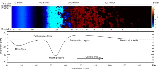
experi-ment for several detector configurations [24]. . . 20 2.11 The top plot shows the time evolution of the 21-cm brightness ,

where the coloration indicates the strength of the brightness. The bottom plot shows the expected evolution of the 21-cm brightness (T21). Note that there is considerable uncertainty due to the

un-known properties of the first galaxies [23]. . . 21 3.1 Exclusion plot for axion-like particles [16]. The left most green

band is the limit obtained by ADMX [42], while the right most green band was obtained by the HAYSTAC [43] experiment. The yellow band shows the KSVZ and DFSZ predictions. The limit . 26 4.1 Diagram showing the three detection processes of dark matter. . . 31 4.2 Diagram of the origin of an annual modulation of the WIMPs flux

[51]. . . 33 4.3 Form factors for different nuclei based on recoil energy [53]. . . 35 4.4 Expected fluorine recoil spectrum (dE/dER) for different masses

of dark matter for a 1 pb cross section: 10 GeV/c2 (black), 20 GeV/c2(blue), 50 GeV/c2(violet), 100 GeV/c2(red), 500 GeV/c2 (green). . . 39 4.5 Schematic of WIMP searches exclusion curves. The region above

the blue curve correspondss to excluded parameter space, while the rest is still allowed. ε denotes the detection efficiencies of dark matter detectors. Typically, ε decreases for low mass WIMPs since they produce lower energy recoils as denoted in the figure (ε < 1_{↓), but ε stays constant for high mass WIMPs.} . . . 40

4.6 Compilation of the WIMP-nucleon cross section limits in the spin-dependent proton sector. The results that are shown are only pub-lished results. The list of all the results and their corresponding references are: PICASSO 2012 (blue) [67], PICASSO FINAL (red) [1], COUPP (teal band) [68], SIMPLE (dashed purple) [69], PICO 2L run2 (green) [70], CDEX (dash black) [71] PICO60 CF3I

(brown, labeled PICO60) [72], PICO 60 C3F8(ndash green) [73],

DarkSide (black) [60], SuperCDMS (dashed orange) [74], Pan-daX (dashed teal) [75], LUX (orange) [76], XENON1T (dash red) [77]. There are also three contours which each represent the possi-ble masses and cross sections that can explain the excess of events seen by the three experiments: DAMA (brown) [78], CoGeNT (magenta) [79] and CDMS-II Si (pink) [80]. . . 45 4.7 Compilation of the WIMP-nucleon cross section limits in the

spin-dependent proton sector. The results that are shown are only pub-lished results. The list of all the results and their corresponding ref-erences are: PICASSO 2012 (blue) [67], PICASSO FINAL (red) [1], COUPP (teal band) [68], XENON100 (orange) [81], SIMPLE (dashed purple) [69], PandaX (dashed red) [82], PICO 2L run2 (green) [70], LUX (dash black) [83] PICO60 CF3I (dash brown,

labeled PICO60) [72], PICO 60 C3F8(brown) [73], IceCube (dash

green) [84], SuperK (dash orange) [85]. The best limit for both in-direct detection (IceCube and SuperK) corresponds to W channel, while the lowest corresponds to b quark channel. . . 46 4.8 The values of the mediator mass (m_med) and the mass of the dark

matter particle (mDM), for which the limit on the WIMP-proton

cross sections are equal, are represented by the black line. The red region represents the limits where production experiments are better than direct detection experiments using superheated liquid detectors. The blue region represents the opposite [91]. . . 49

5.1 Schematic view of the MOSCAB Geyser detector [66]. . . 54 5.2 Phase diagram indicating the region, in dark orange, of the

super-heated state and the stable liquid phase in yellow. The x-axis also shows the critical temperature Tcand the boiling temperature Tb. 55

5.3 Schematic view of the Gibbs free energy as a function of pres-sure. The gradient of each phase is given by the molar volume. A substance always rests in the state with the lowest possible Gibbs free energy. At a phase transition point, the Gibbs free energy of both states is equal as the schematic shows (crossing lines at phase transition points). While the molar volume of the solid and liquid states can be approximated as being constant, this is not the case for the gaseous phase as it is described in the text . . . 57 5.4 Schematic view of the Gibbs free energy as a function of density

and for various pressures. As the pressure is decreased (blue to red), the Gibbs free energy (µl and µv) for both phase, i.e. liquid

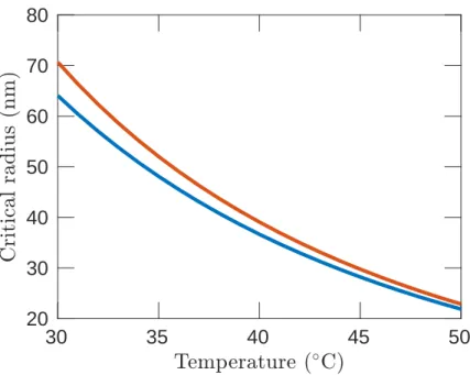
and vapor, decreases, but that of the gas phase decreases more quickly than the liquid phase. Hence, the most stable state become the gaseous phase [99]. . . 59 5.5 Critical radius of C4F10 as a function of temperature at a pressure

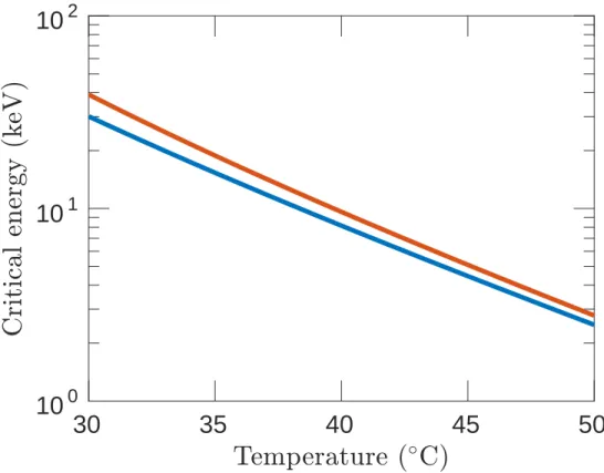
of 1 bar (blue) and 1.2 bar (red) which correspond to the ambient pressure at SNOLAB . . . 63 5.6 Critical energy of C4F10as a function of temperature at a pressure

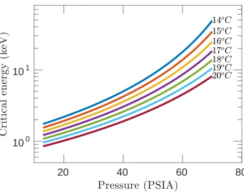
of 1 bar (14.5 PSIA) (blue) and 1.2 bar (17.4 PSIA) (red) which correspond to the ambient pressure at SNOLAB . . . 67 5.7 Critical energy of C3F8as a function of pressure for temperatures

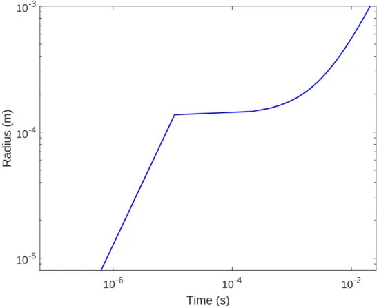
between 14 and 20◦C . . . 68 5.8 Bubble radius time evolution. The linear time evolution

corre-sponds to the inertial regime. The bubble growth evolves into the thermal regime at time t = τ which slows down the growth. . . 70

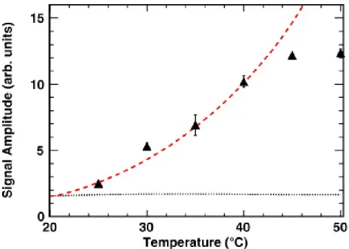
5.9 Time evolution of the acoustic emission. The intensity rises quickly during the inertial regime and then becomes nearly negligible dur-ing the thermal regime. The inflection point corresponds to t = τ . . . 72 5.10 PICASSO detector acoustic amplitude versus temperature at 1 bar

compared to theoretical prediction. The red and black dotted lines represent the acoustic emission in the inertial regime and thermal regime respectively. The theoretical inertial regime replicates the experimental data [108]. . . 73 5.11 Decomposition of the acoustic intensity of the inertial regime for

four freons: C4F10(red) C2H2F4(blue), C3F8(black) and C2ClF5

(green). Each subplot represent one of the quantities enclosed by square brackets in eq. 5.42. . . 74 5.12 Total acoustic intensity versus temperature at a constant 2 keV

en-ergy threshold for C4F10 (red) C2H2F4 (blue), C3F8 (black) and

C2ClF5 (green). The shape of each freon mimics the shape of τ

versus temperature shown in bottom right plot of Fig. 5.11. . . . 75 6.1 Schematic view of a 4.5 L PICASSO detector module. . . 77 6.2 A PICASSO detector module. The drawings show the dimensions

of the containers as well as the position of the piezoelectric sensors [110]. . . 78 6.3 Arrangement of the piezoelectric sensors in the PICASSO

mod-ules. . . 80 6.4 Piezoelectric sensor (left) and acrylic holder (right) of PICASSO

module [110]. . . 80 6.5 Muon flux versus water equivalent vertical depth of the main

un-derground laboratories in the world. The depth of each laboratory is calculated in water equivalent to account for the different rock densities unique to each underground laboratory [112]. . . 81

6.6 Left: One of the eight TPCS of the PICASSO experiment in-stalled at SNOLAB. Each TPCS contains four PICASSO detec-tors. Right: PICASSO experiment setup in SNOLAB. . . 82 6.7 Top: Signal induced by the acoustic emission of a bubble and

recorded by the DAQ. Bottom: FFT of the above signal. The res-onance of the piezoelectric sensor is located at_{≈ 120 kHz.} . . . 83 6.8 The two top (bottom) figures represent the raw and 18 kHz

high-pass filtered amplitudes of a bubble (electronic noise) event. . . . 85 6.9 Graphical representation of the different steps in the construction

of the EVAR variable for a bubble event (left) and electronic noise event (right). Top row: squared signals. Middle row: cumulative sum and linear curve. Bottom row: linear curve subtraction . . . 86 6.10 Comparison between raw signal amplitude (left) and EVAR (right)

distributions. There is no separation between bubble events and electronic noise events in the raw amplitude distribution, but a clear bubble peak is visible on the right side of the red line in the EVAR distribution. . . 87 7.1 Schematic view of a typical PICO detector. . . 89 7.2 PICO60 (left) and PICO40L (right) CAD drawings. The color

band on the PICO40L figure highlight that temperature gradient inside the detector. . . 90 7.3 Typical cycle of a PICO detector. The detector starts in a

com-pressed state at 200 PSIA and followed by an expansion period of a few seconds to reach the desired pressure. When a bubble oc-curs, the pressure system increases the pressure to 200 PSIA, and the detector stays compressed for 30 seconds. . . 93 7.4 PICO60 detector optical simulation of top (left) and bottom (right)

cameras. Each color corresponds to a different sequence of inter-faces. The small +’s are the fiducial markings on the jar. . . 95

7.5 dytranC versus Dwall (top) and Z (bottom). The dytranC>1.3 and abs(Dwall)<15 region corresponds to wall events and is shown in red in the top plot. dytranC < 0.7 and Z > 500 cuts are used to isolate surface events and shown in red in the bottom plot. . . 97 7.6 Dwall event distributions of the cylinder region (top left, main),

collar (top right), hemisphere knuckle (bottom left), and hemi-sphere dome (bottom right). A Gaussian fit is applied to each distribution to place a Dwall cut to the nearest mm beyond 5σ from the mean (dotted red line). . . 98 7.7 Frequency power spectral density squared versus frequency for

av-eraged signals detected for alpha events (red), neutron events (dash blue) and electronic noise events (dash black). The four frequency bands are identified by the green vertical lines. . . 99 7.8 Acoustic Power (AP) distribution for background runs in blue

(al-pha+neutrons) and for AmBe neutron calibration data in red. . . 99 7.9 Left: Picture of the device used to clean the PICO60 jar by rinsing

the jar with UPW and soap (called “dishwasher”). Right: Particu-lates per liter versus particulate sizes for three different standards. The targeted standard (MIL-STD-1246C) is shown in red and was achieved. . . 103 8.1 Top: Theoretical energy spectrum of nuclear recoils for isotropic

scattering in the CM frame. Bottom: the count rate that is mea-sured with a threshold detector. . . 107 8.2 Weighted elastic cross section of (F/C, n) for C4F10 as a function

of neutron energies for the energy range used during detector cal-ibration. . . 108

8.3 Stopping power (dE/dx), calculated with SRIM [118], in units of keV/µm as a function of incident energy for fluorine (dotted), car-bon (dash-dotted) and for α particle (continuous line) in C4F10.

Below 500 keV, fluorine has a higher dE/dx than the other two particles. . . 109 8.4 Simulated range distribution of 3.29 keV fluorine and carbon ions

with SRIM. This energy corresponds to the most recent energy threshold used with the PICO60 C3F8 detector. The range

dis-tribution of fluorine is smaller than carbon which plays a role in bubble formation. . . 109 8.5 Schematic of the internals of a tandem accelerator [120]. . . 110 8.6 Schematic of the Pelletron charging system. This system is

in-stalled in the Montreal Tandem accelerator [120]. . . 111 8.7 Neutron yield of the 51V(p, n)51Cr reaction as a function of

inci-dent proton energy. Resonances allow an excellent definition of neutron energies [121]. . . 112 8.8 The latest version of the PICASSO calibration detector had two

temperature probes as well as two piezoelectric sensors at each end cap. . . 113 8.9 Energy spectrum of simulated 40 keV neutrons just before

inter-acting with the C4F10droplets. The red band represents the energy

threshold that is determined by the operating temperature of the PICASSO detector. . . 114 8.10 Left: CAD drawing showing the bellows, piezoelectric sensors

and the glass jar of the PICO 0.1 detector. Right: Picture of the PICO 0.1 chamber at UdeM inside the thermal water bath. . . 115

8.11 Normalized responses of the monoenergetic neutron beam detec-tor for different incident energies, from left to right: 4 MeV, 2 MeV, 400 keV, 300 keV, 200 keV, 97 keV, 61 keV, 50 keV, 40 keV and 4.8 keV. The five lowest energies were obtained with the reso-nances of the51V (p,n)51Cr reaction and the higher energies with the7Li (p, n)7Be reaction. . . 116 8.12 Energy threshold as a function of C4F10 temperature. The red and

blue triangles shows the different neutron energies produced (left y-axis) with a vanadium target and a lithium target respectively and their corresponding fluorine recoil energy (right y-axis) and their measured critical temperature (x-axis). The black dashed line shows the Seitz threshold energy as a function of the tem-perature at 1 bar, while the black dashed line shows the fit to the data. The210Pb data point (purple triangle) and241Am data point (green triangle) have an energy threshold of 144.1 keV and 71 kev respectively. The details of these alpha calibrations are presented in section 8.7. The energy of the lithium and vanadium data points are, from left to right: 4 MeV, 2 MeV, 400 keV, 300 keV, 200 keV, 97 keV, 61 keV, 50 keV, 40 keV and 4.8 keV. . . 117 8.13 Nucleation probability function used in PICASSO to fit the

cali-bration data. Each curve shows the probability variation for differ-ent α parameters as a function of the energy threshold for a fixed energy recoil. The α parameter used in this plot have the follow-ing values: [0.1,0.5,1,2.5,5,7.5,10,100]. For a higher value of α, the probability reaches 1 faster. . . 119 8.14 Event rate for 61 keV neutrons measured by PICASSO and PICO.

Both data sets were normalized to one another to highlight the similarity of both measurements. The black curve is a fit using the response function from eq. 8.3 with α = 2. . . 120

8.15 Bubble rate as a function of the Seitz threshold measured with the PICO 0.1 detector with a SbBe source that produces 22.8 keV neutrons. The error bars on the y-axis are due to the statistical uncertainty. The sharp increase of count rate at 1.8 keV is due to gamma produced by Sb. . . 122 8.16 Bubble efficiency of fluorine (yellow) and carbon (blue) for 5

dif-ferent probability nodes [0,0.2,0.5,0.8,1]. While the probability node are fixed, their correspoding threshold must be determined by the MCMC. . . 123 8.17 Comparison between the bubble rate multiplicity of GEANT4

sim-ulations and the experimental data taken with the PICO 0.1 detec-tor. The green points are the experimental data points while the blue histograms are the result of the GEANT4 simulations convo-luted with the best bubble efficiency curves found with the MCMC. 125 8.18 Bubble efficiency as a function of recoil energy in keV. The green

band shows the operating Seitz threshold, while the blue and pur-ple bands show the detection efficiency of fluorine and carbon re-coils respectively. The top (bottom) plot shows the bubble effi-ciency for a 2.45 (3.29) keV threshold. . . 126 8.19 35S 17 keV monoenergetic recoil calibration with the PICO 0.1

de-tector filled with C2ClF5. The dashed red line indicates the Seitz

energy threshold of 17 keV while the blue curve shows a sigmoid fit. The uncertainty on the bubble rate is purely statistical while the uncertainty on the energy threshold is due to pressure and tem-perature uncertainties. . . 128

8.20 PICASSO detectors response to alpha decays. The pink curve shows the detector response to the241Am decay chain. 241Am is located outside of the droplets, and therefore only alphas can travel inside the droplets. The blue curve shows the detector response to 144.1 keV recoils produced by the recoils of the daughter nucleus of the214Po alpha decay. . . 130 8.21 EVar distribution for three different energy thresholds; from left

to right: 105.2 keV, 57.9 keV, and 5.1 keV. A second EVAR peak appears due to additional bubbles produce by alpha particles. . . 132 8.22 Acoustic peak ratio between210Pb + alpha (red) and210Pb recoils

(blue) as a function of Seitz threshold. As the threshold decreases the count rate of the second acoustic peak increases and tends to-ward 100%. . . 133 8.23 EVAR count distribution for neutron (red) and alpha decay events

(blue). There is an overlap between the neutron peak and alpha peak. . . 134 8.24 AP frequency spectrum of the first three alpha decays in the226Rn

decay chain: 5.6 MeV (blue), 6.1 MeV (red) and 7.9 MeV (black). It highlights the dependence of AP on the energy of alpha particles. 135 8.25 AP distribution of the PICO 2L detector for two data taking

ses-sions. The AmBe (black) calibration contains both neutron and alpha events, while the dark matter search (red) contains mostly alpha events. The dotted blue line indicates the AP cut defined to reject alpha events while maintaining WIMP sensitivity. . . 136 8.26 Energy shift (∆E) as a function of Seitz energy thresholds obtained

with 17 keV and 144.1 keV calibrations. This way, within the given errors (yellow), ∆E can be extrapolated to the lower PICO operating thresholds. . . 137

8.27 GBS model comparison of 61 keV monoenergetic neutrons. The theoretical curve was normalized to the experimental data. The GBS model shows very good agreement both in C3F8(left, PICO)

and C4F10 (right, PICASSO), and also at other neutron energies. 138

8.28 Gamma nucleation probability of several gamma calibrations per-formed by COUPP, PICASSO, and PICO. The nucleation proba-bility of C3F8at 3.3 keV is equal to∼10−10. Decreasing the Seitz

energy threshold increases the gamma nucleation probability ex-ponentially. . . 139 8.29 Normalized PICASSO detector response to various calibration sources

as well as the response to a theoretical 10 GeV/c2WIMP as a func-tion of the calibrated threshold energy determined with neutron calibration measurements. . . 141 8.30 Neutrino flux energy spectrum [126]. There are three sources:

so-lar, diffuse supernova background (DSNB) and atmospheric. Dark matter detectors are most sensitive to atmospheric and 8B neutri-nos, i.e., high energy neutrinos. . . 142 8.31 ν -Xe elastic scattering event rate as a function of recoil energy

de-posited for the same type of neutrinos shown in Fig. 8.30. A 6 GeV/c2and a 100 GeV/c2WIMP with cross sections of 5_×10−45 cm2 and 2.5_×10−49cm2 respectively are added to highlight the possibility of producing the same signal as 8B and atmospheric neutrino-induced recoils respectively [127]. . . 143 9.1 Graphical representation of the t0finding method based on the

dif-ference between time signal averages of 10 µs (green) and 45 µs (red). The raw signal is shown in blue, and the red dot represents t₀. . . 149

9.2 Vertical distribution of localized bubble events in detector 145 dur-ing WIMP run searches. The distribution should be flat as a func-tion of the vertical distance, but an apparent excess of events his present at the top of the detector. The dotted line represents the physical limit of the detector, and thus several events are recon-structed slightly outside of the detector. In this case, a fiducial cut of z = 6 cm was applied to remove the excess of events at the top of the detector. . . 150 9.3 The count rate (counts/kg/d) of detector #159 for several fiducial

cuts. The count rate without a fiducial cut is shown in black, while the count rate for the benchmark volume (R= 5 cm, Z=_{±8 cm)} is in blue and the final fiducial cut is in red. The error bars are 1σ and only statistical. The count rate of of a fiducial volume must agree with the count rate inside the benchmark volume within 1σ at all temperatures. . . 152 9.4 Count rate versus temperature of AmBe calibration data with WFLVAR

cut (black) and without WFLVAR cut (orange). GEANT4 simu-lated response fitted to each data set is shown as a continuous black line. . . 154 9.5 Vertical event distribution in a PICASSO 4.5 L detector during

neutron calibration for three different source distances. The vari-ous histograms show the bubble height distribution while the solid lines are the fits to the data F(z). The known position of the neu-tron source in the mine is 14.75 cm between the center of a de-tector and the source, and the resulting distribution is shown by the blue curve. This distance can vary between 16 cm and 12.2 cm and the corresponding distribution are shown in black and red, respectively. If not corrected, this effect changes the fiducial mass by 3%. . . 155

9.6 95% acceptance cut for the variable EVAR as a function of tem-perature for two distinct calibration periods of detector 157. The blue and red curves show very similar cut values at 30◦C, but then drift away at 35◦C and 40◦C. . . 157 9.7 Count rate of detector #157 as a function of the Seitz energy

thresh-old after all cuts including the fiducial cut. The purple data points show the experimental count rate while the blue curve is the alpha rate fit. A 10 GeV/c2 WIMP is fitted to the data (red) onto which the flat alpha rate is added to produce the orange curve. The maxi-mum cross section of a WIMP hypothesis compatible with the data is then extracted from the fit. . . 158 9.8 Cross section (picobarn) as a function of the WIMP mass for

de-tector 157. Each data point represents the best WIMP fit for a given WIMP mass. A positive cross section indicates that the count rate increases as a function of the threshold while a decreas-ing count rate would have yielded a negative cross section, i.e., nonphysical cross section. . . 159 9.9 Feldman Cousins statistical analysis used for PICASSO WIMP

searches. The ratio between the cross section and its error (σ /∆σ ) yields different µ values. For a negative value of σ , µ is negative while for positive σ , µ is positive. . . 161 9.10 Compilation of SD WIMP-proton cross section limits at the time

of publication (2012) [67]. . . 162 9.11 Normalized combined weighted average rate versus energy

thresh-old and temperature of 2012 (black) and 2017 (red) datasets. The rate curve of a hypothetical 15 GeV/c2WIMP is shown is blue. . 163 9.12 Summary of the performance of all 32 detectors in term of SD

WIMP-fluorine cross section. The error bars are dominated by statistical uncertainty which comes from the alpha background and decreases as a function of detector number. . . 164

9.13 Upper limits at 90% C.L. on SI-WIMP proton interactions. The fi-nal PICASSO limit is shown as a full red line along with other direct detection experiments: PICASSO 2012 (blue), PICO-2L (green [70]), PICO60 (brown [72]), COUPP-4 (light blue [136]), SIMPLE (dashed purple [69]), CDMSlite (dashed black [137], Su-perCDMS (dashed orange [74]), and LUX (black [138]). The closed countours are the allowed regions of DAMA (brown [78], CoGeNT (magenta [79], and CDMS-II SI (pink [80]. . . 165 9.14 Upper limits at 90% C.L. on SD-WIMP proton interactions. The

final PICASSO limit is shown as a full red line along with other di-rect detection experiments: PICO-2L (green [70]), PICO60 (brown [72]), COUPP-4 (light blue [136]), SIMPLE (dashed purple [69]), XENON100 (dashed light orange [139]) and LUX (dashed black [138]). Indirect searches are represented by Ice-Cube (dashed dark green [140]), SuperK (dashed orange [141, 142]) with comparable limits by ANTARES, Baikal and Baksan [94, 143, 144]. Limits from accelerator searches by CMS are shown in dashed light or-ange [145]. Comparable limits are set by ATLAS [146]. The pur-ple region represents predictions in the framework of the CMSSM [147]. . . 166 9.15 Alpha background rate as a function of detector numbers which

follows the time of fabrication. There is one order of magnitude decrease in the rate between the oldest and newest detector used in the analysis. The alpha background rate is the first source of uncertainty in this WIMP search. . . 167

10.1 Top: Acoustic power (AP) distribution of neutron calibrations (black) and WIMP search data (red). Bottom: Neural network (NN) score versus log(AP) and the corresponding NN score cut of > 0.05 of the same dataset. The AP cuts of 0.5 and 1.5 are displayed in dashed blue in both plots. . . 169 10.2 The 90% C.L. limit on the SD WIMP-proton cross section from

PICO-60 C3F8 plotted in thick blue [73], along with limits from PICO-60 CF3I (thick red) [72], PICO-2L (thick purple) [70], PI-CASSO (green band) [1], SIMPLE (orange) [69], PandaX-II (cyan) [82], IceCube (dashed and dotted pink) [93], and SuperK (dashed and dotted black) [141, 142]. The indirect limits from IceCube and SuperK assume annihilation to τ leptons (dashed) and b quarks (dotted). The purple region represents the parameter space of the constrained minimal supersymmetric model of [147]. Addi-tional limits, not shown for clarity, are set by LUX [138] and XENON100 [81] (comparable to PandaX-II) and by ANTARES [148, 149] (comparable to IceCube). . . 170 10.3 The 90% C.L. limit on the SI WIMP-nucleon cross section from

PICO-60 C3F8plotted in thick blue, along with limits from

PICO-60 CF3I (thick red) [72], PICO-2L (thick purple) [70], LUX (yel-low) [76], PandaX-II (cyan) [75], CRESST-II (magenta) [63], and CDMS-lite (black) [150]. Additional limits, not shown for clar-ity, are set by PICASSO [1], XENON100 [81], DarkSide-50 [56], SuperCDMS [74], CDMSII [62], and Edelweiss-III [151]. . . 172 10.4 SDp limit for various PICO detectors as well as IceCube [93] and

LUX [138]. The PICO40L prediction assumes one year of running at a 3.2 keV energy threshold. The PICO500 prediction assumes 1/4 year of running at 3 keV and 1/2 year at 10 keV. . . 173

11.1 Histogram of the neutron yield (n/ppb/sec/g) of238U as a function of the neutron energy for two different materials: camera (50%Al, 18%H, %17C, %14O), SS and for two different processes: SF and (α,n). The neutron yield produced by (α,n) reactions for the camera material is about one order of magnitude higher than for SS which is mainly due to the presence of aluminum. . . 177 11.2 Block diagram showing each step required to produce GDML

as-sembly files and GDML component files that are ready to use for GEANT4. . . 180 11.3 Left: View of the PICO40L PV which includes the camera ports.

Middle: View of the PICO40L detector without the mineral oil and the plastic shield. Right: PICO40L detector inside the wa-ter bath. The three retroreflector components can be seen and are made of two conical parts and a 180◦hollow cylinder. The central cylinders are the IV, OV, and bellows. The bellows are in between the bellows flanges near the bottom of the central cylinder. The piezoelectric sensors and their cable are also shown. . . 181 11.4 2D plot of the initial positions of the simulated neutrons for the

piezoelectric sensors. There are three stacks of piezoelectric sen-sors, and on each stack, there are four sensors. . . 186 12.1 Transition probabilities for a 4 GeV/c2(top) and 100 GeV/c2

(bot-tom) WIMP for the six possible interactions mentioned in the text. The probabilities are obtained by integrating from 1 keV up to the maximum recoil energy (see eq. 12.15). The left (right)-hand side plot shows the transition probabilities for a pure proton (neutron) coupling. All plots are normalized to 1 with respect to the most responsive target for a given interaction. . . 202

12.2 Schematic view of the nuclear shell model for the proton content. The number of protons in each level for Ge, I and Xe is specified and enters in the estimate of the strength of the spin-orbit coupling. 203 12.3 Transition probabilities for a 4 GeV/c2(top row) and 100 GeV/c2

WIMPs (bottom row) WIMP for the five subdominant interactions (without M). The probabilities are obtained by integrating from 1 keV up to the maximum recoil energy (see eq. 12.15). The left (right)-hand side plot shows the transition probability from a pure proton (neutron) coupling. All plots are normalized to 1 with re-spect to the most responsive interaction for a given target (hori-zontally normalized). . . 204 12.4 Transition probabilities for a 4 GeV/c2 (top) and a 100 GeV/c2

(bottom) WIMP for the six possible interactions. The probabilities are obtained by integrating from 1 keV up to the maximum recoil energy (see eq. 12.15). The left (right)-hand side plot shows the transition probability for a pure proton (neutron) coupling. All plots are normalized to 1 with respect to the Mn. . . 205

12.5 Projected sensitivity of current and future Xe (LUX & LZ) and fluorine based experiment (PICO) in the spin-dependent neutron and proton sector. The corresponding neutrino floor of each active target is shown in gray (Xe) and blue (C3F8). . . 206

12.6 Recoil spectra for WIMP-19F interactions for a 20 GeV/c2WIMP, and for the 5 EFT operators: O1, O3, O4,O8, O11. The spectrum

at low recoil energies is suppressed for some of the EFT operators by the factor ~q2

m2_N in their expression. . . 207

12.7 Recoil spectrum for Xe (red), I (blue), Ge (black) and 19F (ma-genta) for a 20 GeV/c2 WIMP and for the EFT operatorO5. The

solid lines correspond to the M type interaction and the dotted line to ∆. The plot highlights differences in strengths of the two inter-actions M and ∆ for the EFT operatorO5. . . 209

12.8 Limit plot for an isoscalar coupling for the EFT operators O5 for

the latest PICO 60 C3F8, LUX, SuperCDMS and a projected curve

for a PICO 60 filled with CF3I . . . 210

12.9 Isospin limits for the EFT operator O5 for a 100 GeV/c2 WIMP

for PICO 60 C3F8 (red), LUX (black) and a projected curve for

a PICO 60 filled with CF3I (blue). The limits are obtained by

determining c0₅= c5· cos(θ) and c1₅= c5· sin(θ) as a function of

c₅and θ . . . 211 12.10 Destructive interference vector for PICO 60 C3F8(red), LUX

(dot-ted black), hypothetical PICO 60 CF3I (dotted blue), Iodine

(dot-ted pink), Ge (dot(dot-ted brown), Si (dot(dot-ted teal), Na (dot(dot-ted green), along with the isospin limit for LUX (black) and hypothetical PICO 60 CF3I (blue). Iodine and CF3I have the same vector because

flu-orine response is much lower than iodine (see Fig. 12.7) . . . 212 13.1 Right: PICO500 detector inside the pressure vessel. Left: PICO500

detector design at SNOLAB inside the water tank and suspended from a platform. . . 216 13.2 SbBe 22 keV neutron calibration with PICO 0.1 chamber filled

with C2H2F4. Several data set were taken at different

tempera-tures to cover a wide range of energy thresholds. Above _{∼6 keV,} only the elastic neutron scattering of hydrogen atoms can transfer enough energy to produce bubbles. . . 218 13.3 PICO60 projected limit if filled with C2H2F4with an exposure of

1167 kg-day with no background events. The plain line and dotted line are for 1 and 2 keV energy threshold respectively. . . 219 13.4 Detector schematic of the LXe scintillation bubble chamber at

13.5 LAr scintillation bubble chamber. Sensitivity in the SI sector as-suming a 0.1 keV energy threshold for 5 kg-year and 1 ton-year along with current limits (grey) and other projected limits such as NEWS-G, CRESST, DAMIC and SuperCDMS. . . 221 13.6 Number of supernova neutrino events as a function of post-bounce

time for a 725 liters bubble chamber filled with C3F8, CF3I, Ar

WIMP Weakly Interacting Massive Particle MSSM Minimal SuperSymmetric Model

CDM Cold Dark Matter SDp Spin-Dependent proton SDn Spin-Dependent neutron

SI Spin-Independent

MACHO Massive Astronomical Compact Halo Objects LNGS Laboratori Nazionali del Gran Sasso

PV Pressure Vessel IV Inner Vessel OV Outer Vessel

LHC Large Hadron Collider MCMC Markov Chain Monte Carlo

EFT Effective Field Theory AP Acoustic Power

J’aimerais tout d’abord remercier mon directeur de recherche Viktor Zacek de m’avoir donné l’opportunité d’avoir un si grand rôle durant la dernière analyse du projet PI-CASSO. Son encadrement, ses conseils, ses idées et son optimisme ont été source de motivation tout au long de ma thèse. J’adresse également mes remerciements aux mem-bres du jury d’avoir pris le temps de lire cette thèse.

Je voudrais aussi remercier particulièrement mon collègue et ami Wen Chao Chen de m’avoir grandement aidé à l’élaboration et aux vérifications des simulations GEANT4. Je veux aussi remercier Alan Robinson pour son aide et les nombreuses discussions con-cernant le bruit de fond des détecteurs PICO. Merci aussi à Mathieu de m’avoir aidé à apprendre les rudiments de la physique expérimentale et d’avoir été un collègue et un ami tout au long de mes études supérieures. Je souhaite également souligner l’incroyable contribution de Simon qui fut un formidable relecteur/correcteur. Merci à tous les mem-bres présents et passés de la collaboration PICASSO et PICO pour leur contribution aux deux expériences. Merci à tous les étudiants PICASSO et PICO que j’ai côtoyés. Merci à mes collègues et amis du Bunker, Olivia, Fabrice, Merlin, Matthieu, Frédéric D., Frédérick T., Frédéric G., Simon et François pour les nombreuses discussions sérieuses et moins sérieuses.

Je veux également dire merci à ma famille et mes amis pour leur soutien qui m’a été indispensable tout au long de ma thèse. Je tiens à exprimer ma profonde gratitude à mes parents et ma conjointe Sabrina Morel pour m’avoir encouragé de façon incondi-tionnelle.

My contributions to the PICASSO and PICO experiments cover various aspects of both project. For the most part, my work involved performing data analysis as well as Monte Carlo simulations, while also being in charge of several data taking campaigns with the PICO 0.1 calibration chamber.

One of these calibrations consisted of measuring the detector response to 22 keV neutrons with a SbBe source at a 2 keV threshold, which is currently the lowest en-ergy threshold neutron calibration measurement. This measurement is presented in Sect. 8.5.2 of Chap. 8 and is crucial for the determination the WIMP detection efficiency of C3F8at low energy thresholds.

The central part of my work consisted of the analysis of data recorded by PICASSO between March 2012 and January 2014. I was in charge of establishing the WIMP-nucleon cross section limits as well as the fiducial volumes of each of the 32 detectors which required to set novel and strict criteria used to define the fiducial cuts. These fiducials cuts introduced new systematic uncertainties that I had to quantify such as the effect of the position of the source during the neutron calibration.

The second part of my Ph.D. is the interpretation of the role of fluorine in dark mat-ter searches within the context of the Effective Field Theory of dark matmat-ter (EFT). My work consisted in understanding the various theoretical models and to write program-ming codes to compute relevant quantities in order to extract useful information from the models.

One crucial information when searching for WIMPs is the expected background in the detector in particular to neutrons, α, and gamma. My contribution to the future analysis of the PICO40L detector was to predict the neutron background due to the con-tamination of235U,238U, and232Th inside the components of the detector. I performed

simulations of the neutron spectrum produced by each relevant PICO40L components in order to predict the number of single and multiple events per year. Furthermore, I developed a new semi-automatic approach that reduced the time required to include ge-ometrical structures in GEANT4 and greatly decreased the probability of introducing human errors.

INTRODUCTION

Dark matter is an unknown type of matter composed of particles beyond the Stan-dard Model of particle physics. Its presence in the universe is currently known only via its gravitational influence on stars, galaxies, large scale structures of the Universe and on the Cosmic Microwave Background (CMB). Based on the analysis of these observations, the so-called Lambda Cold Dark Matter model or Corcondance Model predicts that 4.9% of the universe consists of ordinary matter, 26.84% of dark matter and 68.47% of dark energy [3]. Dark matter was postulated for the first time in 1933 by F. Zwicky [4] to ex-plain the orbital velocity of galaxies in clusters of galaxies. Since then, several theories beyond the Standard Model of elementary particles have emerged and propose different suitable candidates that respect the various observations. These candidate particles are grouped under the generic name of Weakly Interacting Massive Particles (WIMP) [5]. In particular, one of the emerging models, the Minimal Supersymmetric Standard Model (MSSM), proposes a particle, the neutralino, χ, which is stable, massive, electrically neutral and interacts with matter with a strength of the order of the electroweak interac-tion [6].

The goal of the PICASSO [1]and PICO experiments [2] is to detect dark matter by employing the superheated liquid (SHL) technique, similar to that used in classic bubble chambers. In PICASSO detectors, the SHL is dispersed in the form of micro-scopic droplets of C4F10, while PICO detectors are filled with a bulk fluid of C3F8. The

WIMP-freon interaction consists of an elastic collision between a WIMP and a 19F or

12_{C nucleus, which deposits small amounts of energy in the keV range. These recoil}

nu-clei will then produce phase transitions in the SHL, which is accompanied by an acoustic emission that is captured by piezoelectric sensors. The energy required to induce a phase transition depends on the energy threshold of the SHL which is controled by setting the temperature and operating pressure of the detector, and thus PICASSO and PICO

detec-tors are energy threshold detecdetec-tors that can reach sensitivities as low as a few keVs. The challenge in detecting dark matter lies in the weak strength of the interactions between WIMPs and matter resulting in an expected count rate at a level of 10 events/tonne/year or even smaller. It is therefore vital to build detectors with large active mass to increase the probability of interactions, and to provide the experimental setup with adequate radi-ation shielding against cosmic rays, neutrons, and gammas in order to isolate rare WIMP events.

In this thesis, the observations that proved the existence of dark matter and the de-scription of the several candidate particles in agreement with those observations such as the neutralino will all be described in Chap. 2& 3. There are three possible avenues to detect dark matter, it can be detected indirectly by measuring the decay products of anni-hilating dark matter in the sun or the center of galaxies, it can be produced at accelerator facilities, and lastly, it can be directly detected through WIMP-nucleon interactions in detectors installed in underground laboratories (Chap. 4). All three possibilities will be presented, but since PICASSO and PICO are direct detection experiments using SHL detectors, special emphasis will be put on this technique (Chap. 5 , 6& 7). Another dif-ficulty for dark matter searches is the presence of backgrounds due to Standard Model particles, and thus the extensive calibration measurements performed with neutrons, al-pha particles and gammas will be detailed in Chap. 8.

In 2017, PICASSO published its final WIMP search result and hence a complete chapter is dedicated to the description of the analysis that was performed (Chap. 9). PICO recently published its latest dark matter search with PICO60 (Chap. 10) and the collaboration is currently installing its latest detector, PICO40L. GEANT4 simulations which aim to predict the expected neutron background of PICO40L are described in Chap. 11. Furthermore, the WIMP-nucleon interactions in the context of an Effective Field Theory approach are discussed with an emphasis on the special role of fluorinated targets in the discovery of dark matter (Chap. 12). To conclude this thesis, the current and future activities of the PICO collaboration such as the upcoming PICO500 detector,

the possibility of detecting supernova neutrinos, as well as the possibility to use C2H2F4

DARK MATTER IN THE UNIVERSE

Nowadays, the existence of dark matter is well established, and the most widely accepted explanation regarding its nature is that it is composed of WIMPs (Weakly In-teracting Massive Particle) [5]. Currently, the detection of dark matter and the under-standing of the interaction between baryonic matter and dark matter are among the most active research areas in particle physics. First, in this chapter, the basics of the cosmolog-ical standard model (Lambda-Cold Dark Matter model) will be presented. This model is crucial to the development of any dark matter searches as it proves, beyond any doubt, the existence of dark matter. Then, various measurements highlighting its presence in the Universe will be presented as well as the various possible candidates. A discussion of the MSSM (Minimal SuperSymmetric Model) will follow which offers one possible explanation regarding the nature of dark matter and its interaction with baryonic matter [6].

2.1 Lambda Cold Dark Matter model

The Lambda-CDM model (Cold Dark Matter) is a cosmological model that describes the Universe and is in agreement with the current observations. It starts from the cosmo-logical principle which states that the Universe is homogeneous, i.e., its appearance is the same independently of the position of the observer in the Universe, and is isotropic, i.e., its appearance is independent of the direction of observation. In this model, the equation describing the evolution of the Universe is the Friedmann’s equation which is given by the following expression:

( ˙a/a)2= k/a2+ (8πG/3)ρtot, (2.1)

where a(t) is the scale factor, G is the gravitational constant and ρtot is the density of

Universe:

ρtot= ρM+ ρrad+ ρΛ, (2.2)

where ρMis the total density of matter including baryonic and non-baryonic matter, ρrad

is the density of the radiation and ρΛis the dark energy density. The dark energy density

is a parameter whose addition to the Friedmann equation is allowed by General relativity.

The parameter k describes the curvature of space-time and can take values of +1, 0 or -1 depending on the geometry of the Universe. The first term of eq. 2.1 is the Hubble parameter that represents the expansion rate of the Universe, or, in other words, the rate at which the astronomical objects present in the Universe are moving away from each other. At the present cosmological time, the Hubble parameter becomes Hubble’s constant and is equal to

H₀= h_{· 100kms}−1Mpc−1, (2.3)

where h = 0.6766_{± 0.0042 [3] is a renormalization parameter of the expansion rate. This} renormalization is introduced to relegate the uncertainties of the experimental value to a constant and then the usual values are expressed according to h. A priori, the parameter kthat describes the curvature of the Universe is unknown, however, in the case where k = 0, which means that the Universe is flat, the Friedmann equation makes it possible to obtain the critical density of the Universe, ρc, which is equal to [3]:

ρc=

3H₀2

8πG = 1.05368(11)10

5_h2_{GeV c−2cm−3,}

(2.4)

By using ρc, the relative densities of the components of the Universe are defined by Ωi:

Finally, Ωtot is expressed with the Friedmann equation as:

Ωtot− 1 =

k

H2_a2. (2.6)

In this way, the experimental measurements of Ωtot are directly connected to the

cur-vature parameter k. As an example, if the total density (ρtot) is larger than the critical

density, one obtains an open Universe. Other possible cases are shown in Table 2.I. k = 1 closed ρtot < ρc Ωtot < 1

k = 0 flat ρtot = ρc Ωtot = 1

k = -1 open ρtot > ρc Ωtot > 1

Table 2.I – Possible geometries of the Universe according to the curvature parameter of the space k and the values of ρtot and Ωtot consequently obtained.

2.2 Observational evidences of dark matter

By studying astronomical objects, various inconsistencies between the astronomical models and observations were noted and attributed to the presence of dark matter. These inconsistencies arise from the general properties of dark matter: it is non-radiative and it interacts gravitationally with baryonic matter. In the following sections, the results of astronomical and cosmological measurements proving the existence of the dark matter are presented.

2.2.1 Distribution of galaxy velocities in clusters

The dark matter problem was formed in 1933 following observations of the Coma cluster made by the astronomer Fritz Zwicky [4]. By measuring the speed of galaxies at the periphery of the cluster by Doppler shift and using the Viriel theorem, he estimated its mass. This mass was compared to the visible mass obtained by considering the total number of galaxies contained in the cluster and their respective brightness. He found that the visible mass was 400 times smaller than the mass estimated by the Viriel theorem [7]. This so-called invisible mass required to explain the speed of galaxies far from the

center of the cluster was named "dark matter" by Zwicky.

2.2.2 Rotations curves of spiral galaxies

It was only in the 1970s that a second observation supported the dark matter hy-pothesis proposed by Fritz Zwicky. Vera Rubin measured the speed of hydrogen clouds and stars in the Andromeda galaxy at the periphery and outside the bright region of the galaxy by Doppler shift. She then compared the result with Newtonian dynamics which states that the speed of the stars decreases as a function of their distance from the center of the galaxy if the mass of the galaxy is concentrated in its center. The analysis of the results showed that the speed of the hydrogen clouds remained almost constant as a function of the distance from the center as shown in Fig. 2.1 [8].

Figure 2.1 – Observed rotation speed of the M33 galaxy according to the distance from its center compared to that predicted by the theory [8].

To remedy this inconsistency with the Newtonian theory, Vera Rubin concluded that the galaxy had to contain dark matter in increasing quantity when moving away from the center. The rotational speed of an object in a stable orbit of radius r inside the luminous disk of a galaxy decreases as ν ∝pM(r)/r where M(r) is the mass inside the orbit. In the case where the orbit is located outside of the luminous disk, the velocity goes as ν ∝p(1/r) if all the matter is contained inside of the bright disk. In most galaxies,

on the other hand, the measured velocity remains fairly constant, even out to regions far from the bright center. It implies the existence of a halo of dark matter having a mass density proportional to the inverse of radius squared:

ρhalo∝

1

r2. (2.7)

2.2.3 Gravitational lensing

An important prediction of general relativity applied to astronomy is the modification of the trajectory of the radiation emitted by the celestial bodies. This phenomenon called gravitational lensing effect is divided into two categories; strong and weak. The strong gravitational lensing effect occurs when an object is behind a massive star and its light, from the Earth’s point of view, is curved and produces several images of the same object [9]. Such a phenomenon happens when a quasar, an extremely luminous active galactic nucleus, and a galaxy are on the same line of sight as shown in Fig. 2.2.

Figure 2.2 – Left: diagram of the gravitational lensing effect generated by a galaxy on the image of a distant quasar. Right: the image of a quasar, taken by the Hubble telescope, modified by the gravitational lens effect [10].

Since ordinary matter and dark matter contribute to the curvature of space-time, by measuring the brightness pattern of the distorted image of the quasar, an estimate of the distribution of total (visible + dark) matter around the galaxy is extracted. Thus, knowing where the baryonic matter is located in the galaxy, it is possible to find the contribution

and distribution of dark matter.

The most famous weak gravitational lens phenomenon was observed during the col-lision of the Bullet cluster. When the two sub-clusters collided, the stars of the galaxies were very little affected and were only slowed down gravitationally and their mass was reconstructed using their emitted light. On the other hand, the warm gases interacted strongly which heated them up to 106K such that their emitted X-rays allowed to recon-struct the collision region [11]. Finally, dark matter, which moves freely, is detected by the deformation of the form of the objects in the background by the gravitational lens effect. The result of the collision is shown in Fig. 2.3.

Figure 2.3 – Image of the Bullet Cluster following the collision of two sub-cluster. The hot gas is shown in red, and the presence of dark matter highlighted by the gravitational lens effect is shown in blue [11].

Unlike the strong gravitational lens effect where large distortions of images of astro-nomical objects take place, the weak gravitational lens effect only slightly distorts the images and requires a large number of sources to quantify the mass in the foreground. The light sources will appear larger and flattened, however, galaxies are intrinsically flattened by a factor ranging from 3 to 300 times larger than the flattening caused by the gravitational lens effect depending on the mass in the foreground. It is, therefore,

necessary to have a large number of sources to perform a statistical analysis showing a consistent distortion of the shape of the objects in the background. This analysis was carried out for the Bullet cluster and allowed to reconstruct the location of dark matter in Fig. 2.3. It also determined that the quantity of dark matter must be 49 times larger than the luminous mass observed [11].

2.2.4 Inhomogeneity of the cosmic microwave background

The cosmic microwave background (CMB) is formed of photons released at the age of recombination, 380 000 years after the Big Bang when neutral hydrogen was formed and the Universe became transparent to photons. Today, these photons are present in the form of a characteristic black body spectrum with a temperature of T0 = 2.72548±

00057 K [12] corresponding to a density that is equal to ΩK= 0.0007±0.0019[3].

How-ever, the measurements made to map the sky have revealed inhomogeneities of the order 10−5K which demonstrates that the CMB is not perfectly isotropic as shown in Fig. 2.4 [13].

Figure 2.4 – Map of the celestial sphere showing the temperature fluctuations of the CMB radiation whose origin is from the surface of the last scattering. This measurement was taken by the Planck satellite over five years. The differences of color represent temperature variations of the order of 0.0002 Kelvin [13].

Those anisotropies are the result of quantum fluctuations present before the period of inflation and whose effects are still imprinted in the electron-baryon plasma at the time of recombination. In such a plasma, acoustic oscillations occurred which were due to

the compression of the baryon-photon fluid by gravity and the expansion of the fluid by radiation pressure exerted by the photons [14]. There were regions where the density of baryons was relatively higher than in other regions in which deeper gravitational poten-tial wells were formed. On the other hand, there were regions of lower baryon density where the radiation pressure dominated. These potentials created oscillations of the pho-ton temperature which increases when the plasma contracts and decreases in the opposite case. When photons left the plasma, their temperature was frozen, and thus the photons that were in a potential well with a low density of baryons left with a higher average temperature than those who were in a potential well with a high baryon density. Recent experiences, such as Planck [3] and WMAP [15], measured the temperature differences of the cosmic microwave background at different angular scales. These anisotropies can be analyzed by decomposing them into spherical harmonics whose amplitudes give the angular power spectrum C_lT T which contains the essential information on cosmological parameters such as the densities of each component of the Universe. The amplitude C_lT T is obtained with eq. 2.8 [16]:

CT T_l = 1

(2l + 1)Σ|alm|

2_,

(2.8)

where l represents the order of the multipoles and alm are the amplitude coefficients of

each mode. The temperature power spectrum is given by the following expression:

∆T2=l(l + 1)C

T T l

2π , (2.9)

and is shown in Fig. 2.5 [3]. The first peak appears at l = 200, and its position depends on the curvature of space. If the curvature was negative, the position of the peak would move towards greater values of l without changing the shape of the peak. Thus, the experimental measurements showed that the curvature of space is flat with Ωtot = 1.

Moreover, three additional peaks are distinguishable, and they give information regard-ing the relative amount of dark and baryonic matter. From the height of the first peak one obtains the baryonic density, while the height of the third acoustic peak allows to

infer the relative density of dark matter in the Universe [3]: Ωbh2 = 0.02237± 0.00015, Ωb = 0.04930± 0.00033, ΩDMh2 = 0.1200± 0.0012, ΩDM = 0.2621± 0.0026. 0 1000 2000 3000 4000 5000 6000 D T T ` [µ K 2] 30 500 1000 1500 2000 2500 ` -60 -30 0 30 60 ∆ D T T ` 2 10 -600 -300 0 300 600

Figure 2.5 – Angular power spectrum of temperature fluctuations measured by the Planck observatory. The blue line represents the best fit to the standard cosmological model compatible with a flat Universe [3].

From these results, the proportion of each component of the Universe is presented in the diagram of Fig. 2.6