HAL Id: hal-03232996
https://hal.archives-ouvertes.fr/hal-03232996
Submitted on 23 May 2021
HAL is a multi-disciplinary open access
archive for the deposit and dissemination of
sci-entific research documents, whether they are
pub-lished or not. The documents may come from
teaching and research institutions in France or
abroad, or from public or private research centers.
L’archive ouverte pluridisciplinaire HAL, est
destinée au dépôt et à la diffusion de documents
scientifiques de niveau recherche, publiés ou non,
émanant des établissements d’enseignement et de
recherche français ou étrangers, des laboratoires
publics ou privés.
control
Emmanuel Moulay, Vincent Léchappé, Emmanuel Bernuau, Franck Plestan
To cite this version:
Emmanuel Moulay, Vincent Léchappé, Emmanuel Bernuau, Franck Plestan. Robust fixed-time
sta-bility: application to sliding mode control. IEEE Transactions on Automatic Control, Institute of
Electrical and Electronics Engineers, In press, �10.1109/TAC.2021.3069667�. �hal-03232996�
Robust fixed-time stability: application to sliding
mode control
Emmanuel Moulay, Vincent L´echapp´e, Emmanuel Bernuau, and Franck Plestan
Abstract—This article deals with robust fixed-time stability and
stabilization. First, new global robust fixed-time stability results are proposed for scalar systems by using constant and variable exponent coefficients. Then, they are applied to global robust fixed-time stabilization of a class of uncertain nonlinear second-order systems by using sliding mode control. All the results are illustrated in simulation.
Index Terms—Fixed-time stability, sliding mode control, robust
control.
I. INTRODUCTION
Sliding mode control (SMC) has been developed by Utkin in [1] and then by many authors, see [2] and the references therein for more details. The aim of SMC is to enforce a dynamical system to reach a manifold called “sliding sur-face” defined by a function called “sliding variable” with an appropriate controller ensuring that a constraint on the sliding variable is satisfied. After the constraint is checked, the system trajectories “slide” on the sliding surface towards the desired equilibrium. The main advantage of SMC lies in the simplicity of its feedback control strategy after choosing the sliding variable, its robustness when using discontinuous controllers and the finite-time convergence of the closed-loop system trajectories to reach the sliding surface. Moreover, it has been refined over time, for instance with the integral SMC [3].
Finite-time stability has been developed by Bhat and Bern-stein in [4] and then applied for finite-time stabilization, for instance in [5], [6]. It ensures that dynamical systems reach their equilibrium in a finite-time called settling-time depending on the initial conditions. Finite-time stabilization using a SMC strategy has been developed in [7], [8] where a singularity problem is solved. The fixed-time stability was introduced by Polyakov in [9] and then developed by many authors, for instance in [10], [11], [12], [13], [14]. In addition to finite-time stability, fixed-time stability ensures that the settling-time does not depend on the initial conditions. Fixed-time stabilization provides a predefined convergence Fixed-time
E. Moulay is with XLIM (UMR CNRS 7252), Universit´e de Poitiers, 11 bd Marie et Pierre Curie, 86073 Poitiers Cedex 9, France (e-mail: [email protected]).
V. L´echapp´e is with Amp`ere (UMR CNRS 5005), INSA Lyon, 20 Avenue Albert Einstein, 69100 Villeurbanne, France (e-mail: [email protected]).
E. Bernuau is with GENIAL (UMR INRA 1145), AgroParisTech, 1 Avenue des Olympiades, 91744 Massy Cedex, France (e-mail: [email protected]).
F. Plestan is with LS2N (UMR CNRS 6004), Ecole Centrale de Nantes, 1 rue de la No¨e, 44321 Nantes Cedex 3, France (e-mail: [email protected]).
towards the equilibrium which is a desirable property for engineering applications. In particular, fixed-time stabilization using a SMC strategy with time-independent controllers has been proposed in [15], [16], [17] also by solving a singularity problem. The singularity problem comes from the fact that the simplest finite-time and fixed-time sliding variables are non differentiable. It results in more complex feedback controls to implement. Finally, the notion of predefined/prescribed-time SMC has been introduced in [18], [19], [20] by using time-dependent controllers.
In this article, new global robust fixed-time stability results are provided for scalar systems by using constant and state-dependent variable exponent coefficients. State-state-dependent variable exponent coefficients have already been used in the context of homogeneous self-triggered control in [21]. They have also been used for defining the controllers in [22] for finite-time SMC. But to the best of the authors’ knowledge, it has never been used for fixed-time stability. By employing the SMC strategy, global robust asymptotic stabilization of the global x−system of the state variable x with robust fixed-time stabilization of the s−system of the sliding variable s is obtained by using constant exponent coefficients in the sliding variable and the controllers for a class of uncertain nonlin-ear second-order systems. Moreover, global robust fixed-time stabilization of the global x−system is obtained by using state-dependent variable exponent coefficient in the sliding variable and the controllers. The new sliding mode controllers are time-independent, non singular, robust with respect to bounded disturbances and easy to implement. So using a variable exponent coefficient allows to obtain robust fixed-time SMC of the global x−system contrary to the constant exponent coefficient strategy. Actually, it is not easy to obtain fixed-time stabilization of the global x−system when dealing with SMC because some singularities appear when using the simplest fixed-time sliding variable, see [16] and [17]. With the use of a variable exponent coefficient in the sliding variable and the controllers, we obtain a simple solution because the controllers have no singularity.
The paper is organized as follows. After some preliminaries in Section II, the main results on robust fixed-time stability are given in Section III. The application to SMC is developed in Section IV. Finally, a conclusion is addressed in Section V.
II. PRELIMINARIES
In the following, denoteR+the set of positive real numbers and e the constant such that ln(e) = 1. Recall some results
on finite-time stability and fixed-time stability. Consider the following ordinary differential equation
˙
x(t) = f (x(t)), x(t)∈ Rn (1)
x(0) = x0
with f a continuous function such that f (0) = 0.
Definition 1: [6], [4] System (1) is globally finite-time stable
if it is Lyapunov stable and for all x0 ∈ Rn there exists
T (x0)≥ 0 dependent on the initial conditions such that, for any x(·) solution of (1) with x(0) = x0, limt→T (x0)kx(t)k =
0, i.e. kx(t)k ≡ 0 for all t ≥ T (x0). The function T is called the settling-time.
Definition 2: [9] System (1) is globally fixed-time stable if:
(1) it is globally finite-time stable;
(2) the settling-time function T is upper bounded by a constant T > 0, i.e. for all x0 ∈ Rn, T (x0)≤ T and T does not depend on the initial conditions.
Lemma 1: [9], [14] If there exists a continuously
differen-tiable positive definite radially unbounded function V :Rn→ R+ such that
˙
V (x)≤ −aV (x)γ− bV (x)α (2) where x ∈ Rn, a > 0, b > 0 and 0 < γ < 1 < α, then system (1) is globally fixed-time stable and the settling-time satisfies T (x0)≤ 1 a(1− γ) + 1 b(α− 1). (3) V is called a Lyapunov function for system (1).
In the following, all simulations are performed with a fixed step simulation equal to 0.1ms.
III. ROBUST FIXED-TIME STABILITY
A. Constant exponent coefficient
Consider the following robust fixed-time stability result.
Theorem 1: The system
˙
x =−k1sgn(x)− k2|x|αsgn(x)− k3|x|γsgn(x)− k4x + d
x(0) = x0
(4) with x(t) ∈ R, α > 1, 0 < γ < 1, d(t) ∈ R an external disturbance such that |d(t)| < δ for a given δ > 0, k1 > δ,
k2> 0, k3≥ 0, k4≥ 0 is globally fixed-time stable with the settling-time T satisfying T (x0)≤ 1 k1− δ + 1 k2(α− 1) . (5)
Proof.Consider the following quadratic Lyapunov function
V (x) = x2 (6) Then it leads to ˙ V (x) = −2k1|x| − 2k2|x|α+1− 2k3|x|γ+1− 2k4x2+ 2dx ≤ −2(k1− δ)|x| − 2k2|x|α+1 ≤ −2(k1− δ)V (x) 1 2 − 2k2V (x) α+1 2 (7)
with α+12 > 1. By using Lemma 1, the result follows. Remark 1: On the one hand, the function x7→ |x|γsgn(x) with 0 < γ < 1 is not necessary to obtain the fixed-time
stability while still used for instance in [14], [9]. On the other hand, the sign function x7→ sgn(x) coupled with the function
x7→ |x|αsgn(x) where α > 1 allows the fixed-time stability and is known to reject the disturbances. This is the reason why robust fixed-time stability is obtained. Moreover, if only the first term is used, i.e. if k2 = k3= k4= 0, one only obtains robust finite-time stability.
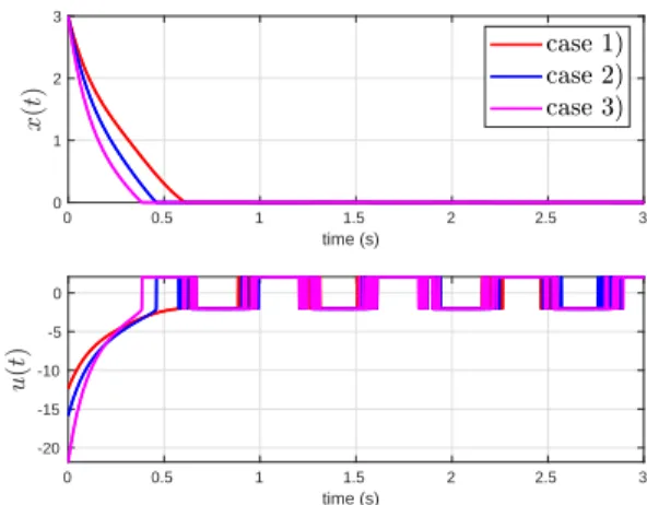
In the following, we compare in simulation the robustness of the state x(t) of system (4) and the term u(t) =−k1sgn(x)−
k2|x|αsgn(x)− k3|x|γsgn(x)− k4x in several cases with the disturbance d(t) = sin(10t) leading to δ = 1, the initial condition x(0) = 3, α = 1.5 and γ = 0.5. Here are the three cases:
• Case 1. k1= 2, k2= 2, k3= 0, k4= 0; • Case 2. k1= 2, k2= 2, k3= 2, k4= 0; • Case 3. k1= 2, k2= 2, k3= 2, k4= 2;
that leads to T (x0) ≤ 2s. Figure 1 shows that system (4) is robust with respect to the disturbance for all cases and Figure 2 shows the induced chattering for the steady state x(t). The settling-time of system (4) in case 3 is strictly lower than the settling-time in cases 1 and 2 because the time-derivative
˙
V is rendered more negative. This explains the interest of
introducing additional terms in system (4) while keeping the robust fixed-time stability.
0 0.5 1 1.5 2 2.5 3 time (s) 0 1 2 3 0 0.5 1 1.5 2 2.5 3 time (s) -20 -15 -10 -5 0
Fig. 1. Top. States x(t) versus time (sec) Bottom. u(t) versus time (sec)
B. Variable exponent coefficient
Consider the following new robust fixed-time stability result using a state-dependent variable exponent coefficient.
Theorem 2: The system
˙ x(t) =−k|x(t)| λx(t)2 1+µx(t)2 sgn(x(t)) + d(t) x(0) = x0 (8)
with x(t) ∈ R, λ > 0 and µ > 0 such that θ = 1+µλ > 1, d(t) ∈ R an external disturbance such that |d(t)| < δ for a
2 2.1 2.2 2.3 2.4 2.5 time (s) -3 -2 -1 0 1 2 3 10 -3
Fig. 2. Zoom on the steady state x(t) versus time (sec)
given δ > 0 and k > δe2eλ is globally fixed-time stable and
the settling-time satisfies
T (x0)≤ 1 (k− δ)(θ − 1)+ 1 ke−λ2e − δ . (9)
Proof. First note that the function φ : x 7→ |x|
λx2 1+µx2 = exp ( λx2 1+µx2ln(|x|) ) is continuous at x = 0 with φ(0) = 1. Therefore the right-hand side of (8) is locally bounded.
Consider the following quadratic Lyapunov function
V (x) = x2. (10) It leads to
˙
V (x) =−2k|x|1+µx2λx2 +1+ 2dx (11)
Consider the case V (x)≥ 1. We have 1+µxλx22 + 1≥
λ 1+µ+ 1 > 2. As |x| ≥ 1 and θ = 1+µλ > 1 it leads to ˙ V (x) ≤ −2 (k − δ) |x|θ+1 (12) ≤ −2 (k − δ) V (x)θ+1 2 (13)
As k− δ > 0 and θ+12 > 1 the proof of [9, Lemma 1] ensures
that all the solutions starting from{V (x) ≥ 1} reaches the set
{V (x) ≤ 1} in a fixed time T1≤ (k−δ)(θ−1)1 . Consider now the case V (x)≤ 1. We have
˙
V (x) =−2k|x||x|1+µx2λx2 + 2dx (14)
As 1 + µx2 ≥ 1 and |x| ≤ 1 it leads to min ( |x|1+µx2λx2 ) ≥ min ( |x|λx2)= e−λ2e and we have ˙ V (x) ≤ −2 ( ke−λ2e − δ ) |x| (15) ≤ −2(ke−λ2e − δ ) V (x)12 (16)
with ke−λ2e − δ > 0. Theorem 4.2 in [4] implies that all the
solutions starting from {V (x) ≤ 1} reach the origin in a uniform time T2≤ 1
ke−λ2e−δ
.
Finally, system (8) reaches the origin in a fixed time
T (x0)≤ T1+ T2.
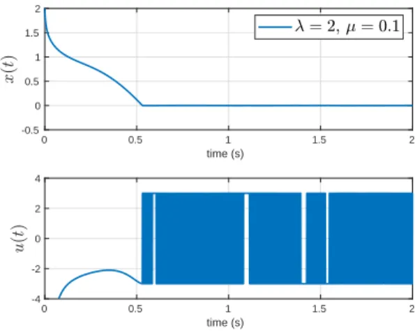
Figure 3 displays the time variations of the state x(t) and
u(t) =−k|x(t)|
λx(t)2
1+µx(t)2 sgn(x(t)) of system (8) with k = 3,
λ = 2, µ = 0.1 and d(t) = sin(10t). As δ = 1, it leads to T (x0)≤ 1.5s . Moreover, a zoom on the steady state x(t) of system (8) is given in Figure 4.
0 0.5 1 1.5 2 time (s) -0.5 0 0.5 1 1.5 2 0 0.5 1 1.5 2 time (s) -4 -2 0 2 4
Fig. 3. Top. State x(t) versus time (sec) Bottom. u(t) versus time (sec)
0.5 1 1.5 2 time (s) -3 -2 -1 0 1 2 3 10 -3
Fig. 4. Zoom on the steady state x(t) versus time (sec)
Remark 2: When x→ ∞, system (8) is equivalent to the
system ˙
x(t) =−k|x(t)|λµsgn(x(t)) + d(t) (17)
with λµ > 1. If λ≈ µ, it is possible to obtain a linear behavior
away from the origin.
When x = 0, given the continuity of x 7→ |x|
λx2
1+µx2,
system (8) is equivalent to the system ˙
x(t) =−k sgn(x(t)) + d(t) (18) which is known to be robust with respect to the disturbances but leads to chattering. This is the reason why high frequency oscillations appears on Figure 3 for u(t); by a similar way
chattering appear on the steady state x(t) of system (8) as shown by Figure 4.
IV. APPLICATION TO SLIDING MODE CONTROL
In this section, consider the following uncertain nonlinear second-order system ˙ x1 = x2 ˙ x2 = f (x) + g(x)u + d (19) with x = (x1, x2) ∈ R2 the state, u ∈ R the control input,
f and g continuous functions such that f (0) = 0, g(x) 6=
0 for all x ∈ R2 and d the external disturbance such that
|d(t)| < δ. The second-order systems have been widely used
in practice, see for instance [23]. The objective is to use the previous results on robust fixed-time stability for designing sliding mode controllers.
A. Constant exponent coefficient
Consider the standard sliding variable
s(x) = x2+ βx1 (20) with β > 0 and the controller
u(x) = −g−1(x) [ f (x) + βx2+ k1sgn(s) +k2|s|αsgn(s) + k3|s|γsgn(s) + k4s ] (21) with k1> δ, k2> 0, k3≥ 0, k4≥ 0, α > 1 and 0 < γ < 1.
Proposition 1: The closed-loop system (19)–(20)–(21)
reaches the sliding surface {s(x) = 0} in a fixed-time satisfying T (s0)≤ 1 k1− δ + 1 k2(α− 1) (22) is also globally asymptotically stable.
Proof. s−dynamics read as ˙s =f (x) + g(x)u(x) + βx2+ d
=− k1sgn(s)− k2|s|αsgn(s)− k3|s|γsgn(s)− k4s + d (23) By using Theorem 1, the first part of the proposition is deduced. When the sliding surface is reached, one has
˙
x1=−βx1 (24) which ensures the asymptotic stability of the closed-loop system (19)–(20)–(21) towards the origin.
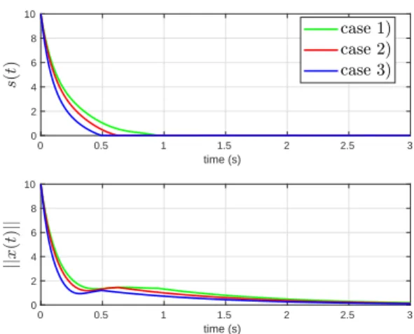
For the simulations, consider the functions f ≡ 0, g ≡ 1,
d(t) = sin(10t), the parameters β = 1, α = 1.5, γ = 0.5, δ = 1 and the gains ki where i = 1,· · · , 4 given by the different cases presented in Subsection III-A. Since all the parameters are the same as in Subsection III-A, one still has
T (s0) ≤ 2s. The time evolution of the sliding variable s(t) and the norms of the state variable kx(t)k associated to the closed-loop system (19)–(20)–(21) are shown on Figure 5.
Remark 3: Let us remark that if system (4) is used for building the simplest fixed-time sliding variable of the form
s(x) = x2+ β1|x1|αsgn(x1) + β2|x1|γsgn(x1) (25) 0 0.5 1 1.5 2 2.5 3 time (s) 0 2 4 6 8 10 0 0.5 1 1.5 2 2.5 3 time (s) 0 2 4 6 8 10
Fig. 5. Top. Sliding variables s(t) versus time (sec) Bottom. Norms of state variable∥x(t)∥ versus time (sec)
with β1 > 0, β2 > 0, α > 1 and 0 < γ < 1 it leads to a singular controller, see for instance [16], [17]. With the classical sliding surface (20), one can get the global robust fixed-time stabilization of the s−system (23), as explained in Proposition 1, but only the global robust asymptotic stabi-lization of the x−system (19). However, the controller (21) is easy to implement. Global robust fixed-time stabilization of the global x−system (19) is obtained in [16], [17] with complex sliding variables and controllers and in the next subsection by using a state-dependent variable power coefficient.
B. Variable exponent coefficient
The main objective of this subsection is to design a new simple sliding variable leading to global robust fixed-time stabilization of system (19). Consider Theorem 2 and the induced sliding variable with a state-dependent variable ex-ponent coefficient given by
s(x) = x2+ β|x1|
λ1x21
1+µ1x21sgn(x1) (26)
with θ1=1+µλ11 > 1, β > 0 and the controller
u(x) =− g(x)−1 [ f (x) + k|s| λ2s 2 1+µ2s2 sgn(s) +βλ1|x1|x2 1 + µ1x21 ( 2 ln|x1| 1 + µ1x21 + 1 ) |x1| λ1x21 1+µ1x21 ] (27) with θ2=1+µλ2 2 > 1, k > δe λ2 2e.
Proposition 2: The closed-loop system (19)–(26)–(27) is
globally fixed-time stable and the settling-time satisfies
T (x0) ≤ 1 (k− δ)(θ2− 1) + 1 ke−λ22e − δ + 1 β(θ1− 1) + 1 βe−λ12e . (28)
Proof. One has ˙s = f (x) + g(x)u(x) +βλ1|x1|x2 1 + µ1x21 ( 2 ln|x1| 1 + µ1x21 + 1 ) |x1| λ1x21 1+µ1x2 1 + d = −k|s| λ2s 2 1+µ2s2 sgn(s) + d (29)
By using Theorem 2, one deduces that system (29) starting at
s(0) = s0 reaches the sliding surface {s = 0} in a fixed-time satisfying T (s0) ≤ (k−δ)(θ1 2−1) + 1 ke−λ22e −δ . From (26), one has ˙ x1=−β|x1| λ1x21 1+µ1x21 sgn(x1). (30)
By using one more time Theorem 2, it is deduced that x1(t) starting at x1(0) = x10 reaches the origin in a fixed-time satisfying T (x10) ≤ β(θ11−1) + 1
βe−λ12e
. Finally, the closed-loop system (19)–(26)–(27) reaches the origin in a fixed-time
T (x0) = T (s0) + T (x10) that is bounded by (28).
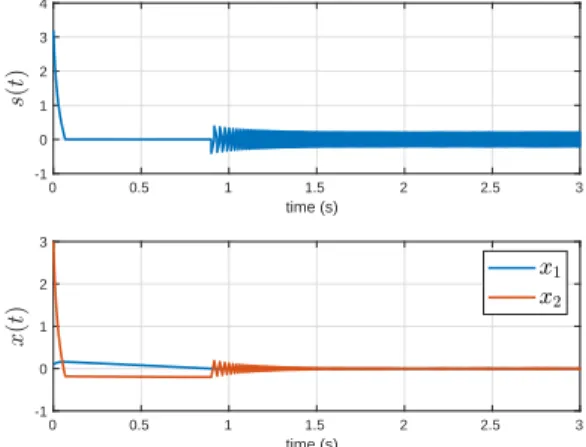
Consider the closed-loop system (19)–(26)–(27) with f = 0, g = 1, β = 0.2, λ1 = 2, λ2 = 4, µ1 = 0.1 µ2 = 1,
k = 10, x(0) = [0.1, x2(0)]T and d(t) = sin(10t). In the case, one gets T (x0) ≤ 13.7s. Figure 6 displays the time evolution of the sliding variable s(t) and the state variable
x(t) = (x1(t), x2(t)). 0 0.5 1 1.5 2 2.5 3 time (s) -1 0 1 2 3 4 0 0.5 1 1.5 2 2.5 3 time (s) -1 0 1 2 3
Fig. 6. Top. Sliding variable s(t) versus time (sec) Bottom. State variable
x(t) = (x1(t), x2(t)) versus time (sec)
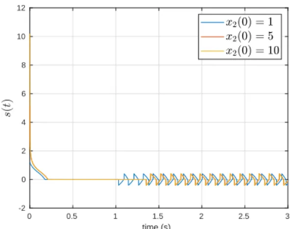
The time evolution of the sliding variable s(t) given by sys-tem (29) is plotted on Figure 7 for different initial conditions
x2(0).
Remark 4: Fist of all, the controller (27) is not singular due
to the fact that limx1→0|x1| ln(|x1|) = 0. Then, if a more simple sliding variable
s(x) = x2+ β|x1|λ|x1|sgn(x1) (31) 0 0.5 1 1.5 2 2.5 3 time (s) -2 0 2 4 6 8 10 12
Fig. 7. Sliding variable s(t) versus time for different initial conditions x2(0)
with β > 0, λ > 0 is chosen and if the controller reads as
u(x) =− g−1(x) [ f (x) + βλ ( x2(ln|x1| + 1) |x1||x1| ) + k|s||s|sgn(s) ] (32) with k > δ then ˙s = f (x) + g(x)u(x) (33) +βλ ( x2(ln|x1| + 1) |x1||x1| ) + d (34) = −k|s||s|sgn(s) + d (35) The fixed-time stabilization is obtained but the controller u(x) is singular due to the fact that limx1→0|x1||x1|ln|x1| = −∞. In order to reduce the chattering induced by the use of controller (27), consider the following controller
u(x) =− g−1(x) [ f (x) + k1sgn(s) + k2|s|αsgn(s) +βλ1|x1|x2 1 + µ1x21 ( 2 ln|x1| 1 + µ1x21 + 1 ) |x1| λ1x21 1+µ1x21 ] (36) with k1> δ, k2> 0, α > 1.
Proposition 3: The closed-loop system (19)–(26)–(36) is
globally fixed-time stable and the settling-time satisfies
T (x0) ≤ 1 k1− δ + 1 k2(α− 1) (37) + 1 β(θ1− 1) + 1 βe−λ12e . (38) Proof.One has
˙s = f (x) + g(x)u(x) +βλ1|x1|x2 1 + µ1x21 ( 2 ln|x1| 1 + µ1x21 + 1 ) |x1| λ1x21 1+µ1x21 + d = −k1sgn(s)− k2|s|αsgn(s) + d (39) By using Theorem 1, one deduces that system (39) starting at
s(0) = s0 reaches the sliding surface{s = 0} in a fixed-time satisfying T (s0)≤k11−δ +k2(α1−1). Then it yields
˙
x1=−β|x1|
λ1x21 1+µ1x2
By using Theorem 2, it is deduced that x1(t) starting at
x1(0) = x10 reaches the origin in a fixed-time satisfying
T (x10) ≤ β(θ11−1) +
1 βe−λ12e
. Finally, the closed-loop sys-tem (19)–(26)–(36) reaches the origin in a fixed-time T (x0) =
T (s0) + T (x10).
The time evolution of the sliding variable s(t) and the state variable x(t) = (x1(t), x2(t)) associated to the closed-loop system (19)–(26)–(36) is plotted on Figure 8 with the same parameters as before and k1= k2= 20, α = 1.5. So one gets
T (x0)≤ 13.5s. 0 0.5 1 1.5 2 2.5 3 time (s) -1 0 1 2 3 4 0 0.5 1 1.5 2 2.5 3 time (s) -1 0 1 2 3
Fig. 8. Top. Sliding variable s(t) versus time (sec) Bottom. State variable
x(t) = (x1(t), x2(t)) versus time (sec)
Remark 5: The use of the sliding variable (26) with a
state-dependent variable exponent coefficient leads to the global robust fixed-time stabilization of the global x−system (19) with the simple controllers (27) and (36) such that the closed-loop system behaves like the standard SMC around the sliding surface. So, a robust behavior of the closed-loop system is obtained similar to the standard SMC but in fixed time. When using system (1) with constant exponent coefficients for building a sliding variable for fixed-time stabilization, the associated controller is singular, see [16], [17].
Remark 6: Note that the proposed fixed-time SMC solution
has the advantage of being simple and easy to tune with respect to the methods presented in [16], [17]. Indeed, our controllers have 6 parameters to tune whereas the controllers in [16] have 14 parameters. In [17], 6 scalar parameters need to be chosen as well as a function to define the sliding surface. The choice of this function is not obvious since it is based on properties of its time-derivative. Finally, both controllers in [16], [17] have a singularity which imposes to use a switched structure and this makes the controller more complex.
V. CONCLUSION
This article deals with global robust fixed-time stability. Several robust fixed-time stability results involving constant and state-dependent variable exponent coefficients are pro-vided and applied to the robust fixed-time stabilization of a class of uncertain nonlinear second-order systems by using
sliding-mode control. For future works, a high order sliding mode strategy could be used for reducing the chattering when dealing with robust fixed-time stabilization.
REFERENCES
[1] V. Utkin, “Variable structure systems with sliding modes,” IEEE
Trans-actions on Automatic control, vol. 22, no. 2, pp. 212–222, 1977.
[2] Y. Shtessel, C. Edwards, L. Fridman, and A. Levant, Sliding mode
control and observation, ser. Control Engineering. Birkh¨auser, 2014. [3] V. Utkin and J. Shi, “Integral sliding mode in systems operating
under uncertainty conditions,” in 35th IEEE conference on decision and
control, vol. 4. IEEE, 1996, pp. 4591–4596.
[4] S. P. Bhat and D. S. Bernstein, “Finite-time stability of continuous autonomous systems,” SIAM Journal on Control and Optimization, vol. 38, no. 3, pp. 751–766, 2000.
[5] Y. Hong, “Finite-time stabilization and stabilizability of a class of controllable systems,” Systems & control letters, vol. 46, no. 4, pp. 231– 236, 2002.
[6] E. Moulay and W. Perruquetti, “Finite time stability and stabilization of a class of continuous systems,” Journal of Mathematical analysis and
applications, vol. 323, no. 2, pp. 1430–1443, 2006.
[7] Y. Feng, X. Yu, and Z. Man, “Non-singular terminal sliding mode control of rigid manipulators,” Automatica, vol. 38, no. 12, pp. 2159–2167, 2002.
[8] S. Yu, X. Yu, B. Shirinzadeh, and Z. Man, “Continuous finite-time con-trol for robotic manipulators with terminal sliding mode,” Automatica, vol. 41, no. 11, pp. 1957–1964, 2005.
[9] A. Polyakov, “Nonlinear feedback design for fixed-time stabilization of linear control systems,” IEEE Transactions on Automatic Control, vol. 57, no. 8, pp. 2106–2110, 2012.
[10] C. Chen, L. Li, H. Peng, Y. Yang, L. Mi, and H. Zhao, “A new fixed-time stability theorem and its application to the fixed-time synchronization of neural networks,” Neural Networks, 2020.
[11] C. Hu, J. Yu, Z. Chen, H. Jiang, and T. Huang, “Fixed-time stability of dynamical systems and fixed-time synchronization of coupled discon-tinuous neural networks,” Neural Networks, vol. 89, pp. 74–83, 2017. [12] S. Parsegov, A. Polyakov, and P. Shcherbakov, “Nonlinear fixed-time
control protocol for uniform allocation of agents on a segment,” in 51st
IEEE Conference on Decision and Control. IEEE, 2012, pp. 7732– 7737.
[13] A. Polyakov and L. Fridman, “Stability notions and lyapunov functions for sliding mode control systems,” Journal of the Franklin Institute, vol. 351, no. 4, pp. 1831–1865, 2014.
[14] Z. Zuo, Q.-L. Han, and B. Ning, Fixed-Time Cooperative Control of
Multi-Agent Systems. Springer, 2019.
[15] A. Levant, “On fixed and finite time stability in sliding mode control,” in 52nd IEEE Conference on Decision and Control. IEEE, 2013, pp. 4260–4265.
[16] Z. Zuo, “Non-singular fixed-time terminal sliding mode control of non-linear systems,” IET control theory & applications, vol. 9, no. 4, pp. 545–552, 2015.
[17] M. L. Corradini and A. Cristofaro, “Nonsingular terminal sliding-mode control of nonlinear planar systems with global fixed-time stability guarantees,” Automatica, vol. 95, pp. 561–565, 2018.
[18] A. Ferrara and G. P. Incremona, “Predefined-time output stabilization with second order sliding mode generation,” IEEE Transactions on
Automatic Control, 2020.
[19] E. Jim´enez-Rodr´ıguez, J. D. S´anchez-Torres, D. G´omez-Guti´errez, and A. G. Loukinanov, “Variable structure predefined-time stabilization of second-order systems,” Asian Journal of Control, vol. 21, no. 3, pp. 1179–1188, 2019.
[20] Y. Song, Y. Wang, and M. Krstic, “Time-varying feedback for stabi-lization in prescribed finite time,” International Journal of Robust and
Nonlinear Control, vol. 29, no. 3, pp. 618–633, 2019.
[21] A. Anta and P. Tabuada, “To sample or not to sample: Self-triggered control for nonlinear systems,” IEEE Transactions on automatic control, vol. 55, no. 9, pp. 2030–2042, 2010.
[22] E. Tahoumi, F. Plestan, M. Ghanes, and J.-P. Barbot, “New robust control schemes based on both linear and sliding mode approaches: Design and application to an electropneumatic actuator,” IEEE Transactions on
Control Systems Technology, 2020.
[23] G. Bartolini, A. Ferrara, and E. Usai, “Applications of a sub-optimal discontinuous control algorithm for uncertain second order systems,”
International Journal of Robust and Nonlinear Control, vol. 7, no. 4,