Redundancy gain: manifestations, causes and predictions
par Sonja Engmann
Département de Psychologie Faculté des Arts et des Sciences
Thèse présenté à la Faculté des études supérieures et postdoctorales en vue de l’obtention du grade de Ph.D.
en Psychologie
option Sciences Cognitives et Neuropsychologie
Avril 2009
Université de Montréal
Faculté des études supérieurs et postdoctorales
Cette thèse intitulée :
Redundancy gain: manifestations, causes and predictions
présentée par : Sonja Engmann
a été évaluée par un jury composé des personnes suivantes :
Martin Arguin Président-rapporteur Denis Cousineau Directeur de recherche Pierre Jolicoeur Membre du jury Aaron Johnson Examinateur externe Stéphane Molotchnikoff Représentant du doyen
A
BSTRACTKeywords: redundancy gain, coactivation, analysis of response time distributions
Response times in a visual object recognition task decrease significantly if targets can be distinguished by two redundant attributes. Redundancy gain for two attributes is a common finding, but redundancy gain from three attributes has been found only for stimuli from three different modalities (tactile, auditory, and visual). This study extends those results by showing that redundancy gain from three attributes within the visual modality is possible. It also provides a more detailed investigation of the characteristics of redundancy gain. Apart from a decrease in response times for redundant targets, these include a decrease in minimal response times and an increase in symmetry of the response time distribution.
This study further presents evidence that neither race models nor coactivation models can account for all characteristics of redundancy gain. In this context, we discuss the problem of calculating an upper limit for the performance of race models for triple redundant targets, and introduce a new method of evaluating triple redundancy gain based on performance for double redundant targets. In order to explain the results from this study, the cascade race model is introduced. The cascade race model consists of several input channels, which are triggered by a cascade of activations before satisfying a single decision criterion,
and is able to provide a unifying approach to previous research on the causes of redundancy gain.
The analysis of the characteristics of response time distributions, including their mean, symmetry, onset, and scale, is an essential tool in this study. It was therefore important to find an adequate statistical test capable of reflecting differences in all these characteristics. We discuss the problem and importance of analysing response times without data loss, as well as the inadequacy of common methods of analysis such as the pooling of response times across participants (e.g. Vincentizing) in the present context.
We present tests of distributions as an alternative method for comparing distributions, response time distributions in particular, the most common of these being the Kolmogorov-Smirnoff test. We also introduce a test yet unknown in psychology: the two-sample Anderson-Darling test of goodness of fit. We compare both tests, presenting conclusive evidence that the Anderson-Darling test is more accurate and powerful: when comparing two distributions that vary (1) in onset only, (2) in scale only, (3) in symmetry only, or (4) that have the same mean and standard deviation but differ on the tail ends only, the Anderson-Darling test proves to detect differences better than the Kolmogorov-Smirnoff test. Finally, the Anderson-Darling test has a type I error rate corresponding to alpha whereas the Kolmogorov-Smirnoff test is overly conservative. Consequently, the Anderson-Darling test requires less data than the Kolmogorov-Smirnoff test to reach sufficient statistical power.
R
ÉSUMÉMots-clés: gain de redondance, coactivation, analyse des distributions de temps de réponse
Les temps de réponse dans une tache de reconnaissance d’objets visuels diminuent de façon significative lorsque les cibles peuvent être distinguées à partir de deux attributs redondants. Le gain de redondance pour deux attributs est un résultat commun dans la littérature, mais un gain causé par trois attributs redondants n’a été observé que lorsque ces trois attributs venaient de trois modalités différentes (tactile, auditive et visuelle). La présente étude démontre que le gain de redondance pour trois attributs de la même modalité est effectivement possible. Elle inclut aussi une investigation plus détaillée des caractéristiques du gain de redondance. Celles-ci incluent, outre la diminution des temps de réponse, une diminution des temps de réponses minimaux particulièrement et une augmentation de la symétrie de la distribution des temps de réponse.
Cette étude présente des indices que ni les modèles de course, ni les modèles de coactivation ne sont en mesure d’expliquer l’ensemble des caractéristiques du gain de redondance. Dans ce contexte, nous introduisons une nouvelle méthode pour évaluer le triple gain de redondance basée sur la performance des cibles doublement redondantes. Le modèle de cascade est présenté afin d’expliquer les résultats de cette étude. Ce modèle comporte plusieurs voies de traitement qui sont déclenchées par une cascade d’activations
avant de satisfaire un seul critère de décision. Il offre une approche homogène aux recherches antérieures sur le gain de redondance.
L’analyse des caractéristiques des distributions de temps de réponse, soit leur moyenne, leur symétrie, leur décalage ou leur étendue, est un outil essentiel pour cette étude. Il était important de trouver un test statistique capable de refléter les différences au niveau de toutes ces caractéristiques. Nous abordons la problématique d’analyser les temps de réponse sans perte d’information, ainsi que l’insuffisance des méthodes d’analyse communes dans ce contexte, comme grouper les temps de réponses de plusieurs participants (e. g. Vincentizing).
Les tests de distributions, le plus connu étant le test de Kolmogorov-Smirnoff, constituent une meilleure alternative pour comparer des distributions, celles des temps de réponse en particulier. Un test encore inconnu en psychologie est introduit : le test d’Anderson-Darling à deux échantillons. Les deux tests sont comparés, et puis nous présentons des indices concluants démontrant la puissance du test d’Anderson-Darling : en comparant des distributions qui varient seulement au niveau de (1) leur décalage, (2) leur étendue, (3) leur symétrie, ou (4) leurs extrémités, nous pouvons affirmer que le test d’Anderson-Darling reconnait mieux les différences. De plus, le test d’Anderson-Darling a un taux d’erreur de type I qui correspond exactement à l’alpha tandis que le test de Kolmogorov-Smirnoff est trop conservateur. En conséquence, le test d’Anderson-Darling nécessite moins de données pour atteindre une puissance statistique suffisante.
C
ONTENTSABSTRACT ... iii
RÉSUMÉ ...v
CONTENTS ... vii
List of tables ... xii
List of figures ... xiii
List of abbreviations...xv
Dedication ...xvi
Acknowledgements ... xvii
CHAPTER 1: Introduction ...1
Analysis ...6
Threshold of race model performance...6
Miller Inequality ...6
Townsend Bound...8
Differentiating between response time distributions ...11
Empirical data...15
Pilot experiment A (3RedA)...15
Method ...15
Results...20
Further research: General method ...25
Practice effects...27
Effects of masking...32
3RedC : Masked...32
2RedM&M : Masked / Unmasked...36
Early processing stages...39
3RedD : colour, orientation, frequency...40
3RedDSat : low saturation...44
3RedE1 : colour, form, and movement ...45
Do certain brain areas favour coactivation? ...46
2RedMST : perceived depth and direction of movement ...47
Characteristics of redundancy gain ...53
Modelling ...55
Final research questions ...57
CHAPTER 2: Coactivation results cannot be explained by pure coactivation models...58
Déclaration des coauteurs...59
Apport original ...60
Abstract ...61
Introduction ...62
Method...71
Participants ...71
Stimuli and Apparatus ...71
Procedure...73
Results ...75
Difference in negative contingencies ...76
Redundancy gain ...77
Excluding Race Models...80
Excluding race models for gain from double to triple redundancy ...83
Characteristics of the RT distributions ...86
Predictions of the coactivation model ...89
The cascade race model...92
The serial coactivation model...94
The parallel coactivation model ...96
Some conclusions related to model fitting ...100
Discussion ...102
Acknowledgements ...109
References ...110
Appendix A: Simulating the coactivation model ...120
Tables ...122
Figures ...127
CHAPTER 3: Comparing distributions: the two-sample Anderson-Darling test as an alternative to the Kolmogorov-Smirnoff test...138
Déclaration des coauteurs...139
Abstract ...141
Introduction ...142
Why combining response time distributions across participants is problematic ...143
Different methods of comparing distributions participant-by-participant..144
Comparison of Kolmogorov-Smirnoff and Anderson-Darling tests...148
Kolmogorov-Smirnoff Test ...148
Anderson-Darling Test ...150
Comparison of the two tests when shift, scale and symmetry are varied independently ...153
Method ...154
Results...155
Comparison of the two tests when D1 and D2 differ in the tails only...158
Method ...158
Results...159
Sample size needed to reach sufficient statistical power when shift, scale and symmetry are varied independently...159
Method ...161 Results...161 Discussion ...164 Acknowledgments ...166 References ...167 Appendix ...172
Tables ...174
Figures ...177
CHAPTER 4: Conclusion...183
GENERAL REFERENCES...186
APPENDIX ...195
List of tables
CHAPTER 1
Table I. Stimulus distribution for one block for three target attributes...19
CHAPTER 2
Table 1. Stimulus distribution for one block of 60 trials ...122 Table 2. Proportion of participants for whom the distribution in a condition
was significantly different from the distribution in a condition with less redundancy ...123
Table 3. Summary of the various predictions made by race models...124 Table 4. Fit of the models to the response time distributions of the correct
response ...125
Table 5. Mean fit and mean parameter values for the models tested ...126
CHAPTER 3
Table 1. Parameters of the Weibull and Normal distributions...174 Table 2. Definition of large, medium and small effect size for the three
parameters of the Weibull distribution...175
List of figures
CHAPTER 1
Figure 1. Examples of stimuli...18
Figure 2. Experiment 3RedA...22
Figure 3. Experiment 3RedB ...30
Figure 4. Experiment 3RedC ...35
Figure 5. 2RedM&M: effect of condition and masking on response times.38 Figure 6. Experiment 3RedD...43
Figure 7. Examples of stimuli for the experiment 2RedMST ...49
Figure 8. Experiment 2RedMST ...52
CHAPTER 2 Figure 1. Mean response time per condition. ...127
Figure 2. RT distributions of participant 13 for single- and double redundant conditions...128
Figure 3. RT distributions of participant 13 for double and triple redundant conditions...129
Figure 4. Townsend Bound and RT distributions of participant 13 for double redundant conditions ...130
Figure 5. Townsend Bound and RT distributions of participant 13 for triple redundant conditions...131
Figure 6. Townsend Bound and Townsend Bound calculated from double redundant distributions...132
Figure 7. Parameters of RT distributions...133 Figure 8. Parameters of RT distributions – real and simulated ...134 Figure 9. Different versions of a race model with three possible inputs ...136 Figure 10. Influence of the parameters ρ (internal redundancy), R (external
redundancy) and k (decision threshold) on the observed
symmetry...137
CHAPTER 3
Figure 1. The proportion of significant differences between the two
distributions for the AD and KS test as a function of Δ1 (changes in shift) ...177 Figure 2. Absolute advantage of AD over KS test as a function of Δ1
(changes in shift)...178 Figure 3. The proportion of significant differences between the two
distributions for the AD and KS test as a function of Δ2 (changes in scale) ...179 Figure 4: The proportion of significant differences between the two
distributions for the AD and KS test as a function of Δ3 (changes in asymmetry) ...180 Figure 5. Weibull and Normal distributions used for evaluation of
performance when distributions differ at tails ...181 Figure 6. The two distributions compared when the effect size of change in
List of abbreviations
AD test Anderson-Darling test °VA degree of visual angle KS test Kolmogorov-Smirnoff test
ms milliseconds
P probability RT response times RTE Redundant Target Effect std standard deviation
Acknowledgements
First and foremost, I would like to thank my supervisor, Denis Cousineau. His support - professional, financial and moral - through experimental and statistical problems, visa troubles and loss of motivation, has been greatly appreciated, and this thesis wouldn’t have been possible without it.
My colleagues, especially Jade Girard and Sophie Callies, have made my studies so much more enjoyable and fun. I would like to thank them for the numerous animated discussions, lunch breaks in company of M Hubertu, and all other moments of procrastination we shared.
The encouragement and support of my friends has been invaluable. I want to thank in particular: The Rhizome, for its warmth, colourfulness and craziness, for being my home, for providing the balance to sitting in front of a computer; the Coop sur Genereux, for feeding me and letting me crash; Zbyněk, for Hostyn, for always being there, and listening patiently to the latest developments in my thesis.
And finally, I am very grateful for the continued support and love of my parents and brother. They have given me the freedom and strength to become the person I am today. And they have been very patiently waiting for me to finally finish my studies!
C
HAPTER1
I
NTRODUCTIONRecognizing objects is a seemingly simple, even trivial task to ask of a human. However, when trying to disassemble the process of object recognition into its different components, or trying to simulate human performance on object recognition tasks, we quickly realize that it is far more complex, and that we are still far from understanding why humans perform so well, and far from achieving close to human performance in models of object recognition.
Visual input is decomposed into its smallest parts (single neuron receptive fields) by the visual processing system. Visual processing is organised in a hierarchical manner, with a series of subsequent processing areas analysing more and more complex combinations of information (Goodale & Milner, 1992; Kandel, Schwarz & Jessell, 2000). Complex objects can either be processed holistically (such as faces; Desimone, 1991; Farah, 1990) or analytically, that is by analysing the constituent parts (Farah, 1990; Biederman, 1990). However, we do not know how complex objects are reconstituted from their individual components. How does the visual system know which features belong together? This problem is referred to as the binding problem (Treisman & Gelade, 1980, Treisman, 1996). Several possible solutions for the binding problem have been proposed including the ‘grandmother cell theory’, which postulates highly specialised cells that respond to a specific combination of attributes (Barlow, 1972), spatial proximity
(Wolfe, Cave & Franzel, 1989), and the theory of synchronized firing of cells responding to the same object (Milner, 1974; Singer & Gray, 1995). Although the debate is not resolved yet, a combination of combined selectivity, synchronized firing and spatial proximity seems most likely to account for binding of objects (Treisman, 1996).
Spatial proximity, perceived continuity, or similarity of features can account for what is perceived as an object (Treisman, 1990; Palmer, 1981; Gestalt Psychology: Köhler, 1947, among others). This is generally known as an effect of grouping. Contrast also plays a major role in object recognition. It is the most important and most studied tool for defining what constitutes an object, where the edges of an object are (Marr, 1976), and what belongs to another object or background (Lamme, 1995). Our visual system is based upon an analysis of contrast (e.g. luminance contrast, colour, motion or orientation contrast; Livingstone & Hubel, 1988), and contrast plays an important role in the attraction of attention (Engmann et al., in press). Contrast is frequently high around the edges of objects (e.g. there is a difference in colour between an object and its background), and it has been shown that high contrast attracts fixation (Tatler, Baddeley & Gilchrist, 2005) and that the visual cortex responds selectively to objects that are separated from the background by elevated high contrast (Zipser, Lamme & Schiller, 1996; Lamme, 1995).
Object recognition can be facilitated or inhibited by a number of factors, such as familiarity or complexity of the object (Logothetis & Sheinberg, 1996),
familiarity of viewing angle (Tarr & Pinker, 1989), or context (Torralba, Murphy, Freeman & Rubin, 2003). Another characteristic that can facilitate or inhibit object recognition involves the number of target attributes by which an object can be recognised. In certain situations, several distinct attributes that indicate the identity of an object can facilitate object recognition, in other situations, object recognition is inhibited by several target attributes. If a target object is defined by a single attribute that separates it from its surroundings, recognition is facilitated independently of the number of surrounding distracters (Pop-out effect; Treisman & Souther, 1985). If a combination of attributes is needed to unambiguously identify a target (i.e. if the target itself is unique, but shares at least one feature with all surrounding distracters) target recognition is inhibited and becomes dependent on the number of distracters (Treisman & Souther, 1985). However, if a target is defined by a combination of attributes, either of which is sufficient to identify the target, recognition is facilitated. This is known as the redundant target effect (RTE; Kinchla, 1974; Miller 1982). Chapter two contains a review of literature on the RTE, the main body of which studies objects defined by two target attributes. Stimuli defined by three target attributes have rarely been studied (Diederich, 1995), and never within a single modality. An investigation of triple redundancy gain in purely visual stimuli is a novel question.
The initial motivation for the present study was to provide evidence for triple redundancy gain in the visual modality. The main goal was to show that within one modality, redundancy gain is not limited to two features, but that each new target feature added has a facilitatory effect on object recognition. We also
wanted to investigate for which feature combinations a triple redundancy gain is possible. A combination of three visual target features that produces a significant gain in reaction time speed over double redundant targets is therefore sought.
The question of a possible generalisation from a “double” RTE to a “triple” RTE is a very important one. An in-depth investigation would shed much light on information processing within a single modality. It has been shown that the RTE is only possible when parallel processing is assumed (Van der Heijden, La Heij & Boer, 1983, Krummenacher, Müller & Heller, 2001). The absence of additional gain from a third target attribute would, for instance, demonstrate a limit of parallel processing in the visual system. Therefore, the first important question is whether enough resources can be made available for a single modality to process three features in parallel quickly enough to enable a redundancy gain from the third attribute.
Another motivation for this study was to clarify the question of possible causes of redundancy gain (again, chapter two contains a more detailed review of different theories). Several types of models have been proposed to explain the RTE, namely the race model (Raab, 1962), the coactivation model (Smith, 1968; Miller 1982; Schwartz, 1989) and crosstalk (Mordkoff & Yantis, 1991). Race models assume independent channels separately accumulating evidence in favour of the specific signal or feature to which they are tuned. Object recognition occurs when one channel has accumulated enough evidence to overcome its decision threshold. Race models allow redundancy gain because more channels improve the
chances of evidence for one feature being accumulated particularly fast. This probability-based explanation of the RTE allows the calculation of an upper limit to performance of race models (Miller 1982). Coactivation models combine evidences from different channels to satisfy a single threshold criterion. If several channels exist, the pooling of activation from several still weakly activated channels will be sufficient to overcome the threshold, thereby causing redundancy gain. Crosstalk models are basically race models with connections between channels, allowing benefit from correlations between different features, and thus causing a redundancy gain.
The goal of this study was to provide experimental data that is able to distinguish between three different theories explaining the RTE in the visual system, and thereby to exclude two out of three of these possible explanations, either a priori, through the experimental design, or a posteriori, by the use of a decision criterion definitely favouring or excluding one theory based on the experimental results. We hypothesized that coactivation is the rule in the visual system, but might not always be directly observable due to different noise levels, or different processing speeds as a function of the visual features involved.
Analysis
The research goals formulated above posed two methodological problems for the analysis of response time data. First, we had to define a threshold of race model performance for triple redundancy. Second, we needed to find an appropriate statistical test for finding differences between response times from different conditions without losing information.
Threshold of race model performance
Miller Inequality
To provide evidence in favour of or against race models as a cause for gain, most recent studies investigating redundancy gain and coactivation models used the Miller Inequality (Miller, 1978),
(1)
where P(TR<t|Ti) is the probability of participants responding faster than time t
given a target (Ti) is present on channel i.
It is conceivable that two feature channels are not independent of each other. Since this dependency can stem from any number of possible causes, many of which could be biological and therefore not directly observable, one cannot estimate the degree of dependence between channels. All one knows is that it must
be equal to or greater than zero. If X equals the degree of dependency between two channels,
(2)
then X needs to be subtracted from the sum of response time distributions of the separate channels to calculate race model performance for two redundant channels:
(3)
Subtracting X, an unknown positive quantity, from both sides of the equation leaves us with the Miller Inequality (eq. 1), a definite upper limit to the performance of race models with two channels, and a very efficient criterion of exclusion for race models on any task with two redundant targets.
When generalising equation (3) to three channels, we need to factor in dependencies between any two channels
(4)
and all three channels,
(5)
(6)
The degree of dependency between all three channels, Y123, an unknown
positive number, is a subset of each Xij, and therefore, having been subtracted
thrice with each Xij, needs to be added twice to the equation again to make it valid.
Both types of dependencies are of unknown positive size, so trying to factor them out of equation (6) makes it impossible to determine in which direction the extension of the Miller Inequality would tend.
Diederich and Colonius, in their 2004 study, used an extension of the Miller Inequality to three channels to refute race models in a stimulus detection task with stimuli from three different modalities (auditory, visual, and/ or tactile). Their extension is not valid for this study, however, since it did not account for the unknown factor of dependency between all three channels, and we cannot assume three channels from a single modality to be completely independent of each other.
Townsend Bound
An alternative to the Miller Inequality was proposed by Townsend and Nozawa (1995; a similar bound was proposed by Mordkoff and Yantis, 1991, p. 535). It is based upon survivor functions (one minus the cumulative distribution) of response times instead of cumulative distribution functions. The upper limit to race model performance with more than one channel is given by the survivor function of the product of the survivor functions of each channel:
(7)
where RT123 is a response time when target attributes from all three channels are
present and i indexes the three channels. If the observed response time distribution in a redundant target task is significantly faster than predicted by this boundary, race models as the sole explanation of redundancy gain are rejected. The Townsend Bound can be calculated for any number of channels.
For a pure race model, the Townsend Bound for three channels based on the three survivor functions of the single channels is perfectly valid. However, we need to consider the possibility of a mixed coactivation and race model being able to explain the results. What if a decision about object identity was made coactively by two channels, but the third channel contributes solely on a winner-take-all basis? So the question is: how do we distinguish between the possibility of a mixed model and a pure coactivation model (i.e. a model where responses from all three channels are pooled to satisfy a single decision criterion)? We calculated a Townsend Bound for mixed models (models where two channels interact by coactivation and the third channel contributes only within the range of statistical facilitation) based on the survivor functions of an RT distribution where target attributes are present on two channels plus the RT distribution of the target attribute on the respectively missing channel. This yields three Townsend Bounds (one for each combination of two plus one channels), which we combine into one
single threshold criterion for mixed models by taking the maximum value out of these three criteria at each time point:
(8)
This yields the most liberal evaluation of performance if any of the three channels contributes only by statistical facilitation as a third redundant attribute. Hence, exceeding the limit can only be achieved if all three target attributes contribute significantly by coactivation to the amount of redundancy gain. Alternatively, the Townsend Bound for mixed models could have been calculated from the product of the survivor functions of response times in the three possible conditions when target attributes on any two channels were present, analogous to equation (7). However, in this case, the gain contributed by each attribute would be included twice (once in each of the two double redundant conditions it is part of), thereby obtaining an upper limit which would definitely exceed performance of a combination of coactivation for two and statistical facilitation for the third attribute. Equation (8) ensures that each attribute contributes only once, while still ensuring the best possible performance under the assumption that statistical facilitation is responsible for the gain attributed to the third target attribute.
When testing for triple redundancy, we used the simple Townsend Bound (eq. 7) as a default. Should it be violated, we also tested violation of the mixed-model Townsend Bound (eq. 8).
Differentiating between response time distributions
We decided to analyse response time data on a participant by participant basis for various reasons, mainly because grouping of several participants’ response time data is invariably accompanied by some loss of information – information about variance and symmetry which is particular to individual participants. This leads to false representations of RT data, such as flattened or bimodal distributions, which tend towards normality, even if the underlying individual response time distributions are not normally distributed. Using a technique such as Vincentizing (Vincent 1912, Rouder & Speckman, 2004) for grouping avoids bias due to loss of variance information. Vincentizing involves grouping RT distributions by quantiles: response times in the first nth percentile of each RT distribution are averaged, and response times in the next nth percentile,
and so on. Distributions are “averaged” by taking into account the relative position of each response time, thereby avoiding flattening or bimodality. However, Vincentized distributions still tend towards normality (Thomas & Ross, 1980), whereas normality cannot be assumed for response time distributions (Logan, 1992; Rouder, Lu, Speckman, Sun & Jiang, 2005).
Several authors used multiple t-tests on quantiles (Miller, 1982; Mordkoff & Yantis, 1991, 1993, among others). Quantiles (e. g. the 5th percent quantiles) are computed for each participant in the two conditions whose distributions are to be compared, and then tested for equality using a t-test. This procedure is replicated for all quantiles at given intervals (e. g. the 10th, the 15th, etc. percent). This
method allows an estimate of where RT distributions of all participants differ significantly. It keeps individual participants’ data separate, and analyses more than distribution means.
However, we noticed a large between-participant variability in all our experiments (see next section), the difference between participants being at times larger than the actual effect of redundancy gain. In this case, multiple t-tests cannot detect redundancy gain. Additionally, sample size for each t-test is only as large as the number of participants in an experiment; therefore statistical power may not be sufficient, especially if the effect size is not very large to begin with. Finally, the data at one time point are highly correlated with the data at the previous and following time point, influencing the probability of a type I error. We therefore decided upon a participant by participant analysis.
An analysis of redundancy gain on a participant by participant basis has the advantage of keeping all information particular to a participant, while making the effect of redundancy gain directly observable, without having to factor out between-participant variability. The most common methods of comparing response time distributions, a t-test or an ANOVA, were not an option for analysis, since both assume normality, and only analyse differences in mean and variance of samples. Therefore, the best choice for a participant by participant analysis of response times in the present experimental context is a test of distributions, the most well-known being the Kolmogorov-Smirnoff (KS) test (Kolmogorov, 1941; Smirnoff, 1939). The Anderson-Darling (AD) test (Anderson & Darling, 1952), an
alternative similar to the KS test, is mainly used in the field of engineering and not known in psychology at all.
We implemented a two-sample version of the AD test in Matlab (MathWorks Inc., Natick, MA). After comparing the performance of the KS and the AD test on our experimental data, we noticed that the AD test was more sensitive to small differences between response time distributions. Also there is evidence that the one-sample version of the AD test is especially sensitive to the tail ends of distributions (Darling, 1957). If this holds true for the two-sample version as well, the AD test is even better suited to the current context: we hypothesize that minimal response times are more affected by redundancy than other characteristics of response time distributions. We suspect that the two-sample AD test is a powerful tool for comparing response time distributions, and should be more frequently used in the field of cognitive psychology. After implementing the two-sample version, we therefore decided to test power and reliability of the AD test more rigorously. At the same time this gave us an opportunity to review other techniques for analysing response time distributions (see chapter three for details).
In order to determine which test was more powerful and better suited to the present context, we calculated the probability of both the AD test and the KS test to detect differences in shape, symmetry, shift and behaviour at the extrema of samples drawn from theoretical distributions in a series of Monte Carlo simulations. These are four additional ways, apart from mean and variance, to
characterise response time distributions (especially if these aren’t normally distributed). We relied on all this additional information in order to differentiate between response time distributions, and needed the test most adapted to detecting differences in all these dimensions. Also, due to the participant by participant analysis, the amount of data per condition was not very large in most of the subsequently described experiments. We therefore also needed to determine which test would yield greater statistical power (Cohen, 1992) given the expected effect size. The Anderson-Darling test proved superior on the detection of differences between distributions as well as for statistical power. Please refer to chapter three for details of method and results of Monte Carlo simulations and the calculation of statistical power.
Empirical data
The following section provides a description of the progression of this research, and the subsequent evolution of the research questions. A series of pilot experiments were necessary in order to develop the paradigm for the last, successful experiment described in chapter two. Each of these pilot experiments provides interesting results, such as empirical evidence that parallel processing is needed to observe a redundancy gain (2RedMST), or the effect of practice (3RedB) and masking (3RedC and 2RedM&M) on the redundancy gain. This section can be skipped without compromising the comprehension of the remaining chapters.
Pilot experiment A (3RedA)
Method
Participants. Participants were 4 female undergraduate students from the
Université de Montréal, between 19 and 25 years of age. All had normal or corrected-to-normal vision. Participants were compensated with 8$ per hour for their participation.
Stimuli and apparatus. We used simple two-dimensional geometrical
objects as stimuli. Stimuli were created in the RGB color space, using Matlab (MathWorks Inc., Natick, MA). Stimuli were presented using E-Prime (Psychology Software Tools, Inc., Pittsburgh, PA) on a SVGA monitor (refresh rate: 85 Hz) at a distance of 80 cm from the participants. The stimuli measured 1.5,
2 or 3 °VA (degrees of visual angle); they were either red, green, or blue; and lastly, their form was a circle, a triangle or a square (see Figure 1 for an example of the stimuli used). Stimuli were presented in front of an equiluminant gray background with stimulus luminance at 50% and stimulus saturation at 100% percent. Target stimuli possessed one or more of the following attributes: color red, form of a circle, and medium size (2 °VA). The presence of any single one of these attributes was sufficient to define a given stimulus as a target. Non-target stimuli did not possess any of the target attributes. They were either green or blue, a triangle or a square and large or small in size.
Design. 50% of all stimuli presented to participants were targets. To avoid
contingencies between attributes on different channels which would facilitate redundant target recognition, the stimulus distribution shown in Table I (top) is an extension of the distribution suggested by Mordkoff and Yantis (1991), following the three rules of contingency formulated by Mordkoff and Yantis (1991).
Procedure. The experiment consisted of 17 blocks with 42 trials per block
for a total of 714 trials. Stimulus distribution did not vary between blocks, but the order of trials was randomized. Participants had the possibility to take a break between blocks. The triple redundant target (target with all three target attributes present), the three double redundant targets (any two target attributes present, plus one of two possible distracters on the third channel), and the three stimuli with only one target attribute present, were presented 51 times per participant. Non-target stimuli were presented 357 times per participant. Each trial started with the
presentation of a fixation point for 850 ms. The stimulus was then presented for 1000 ms. Finally, a feedback slide appeared for 1200 ms, which was followed by a blank screen for 1000 ms in preparation for the next trial.
We used a Go-NoGo experimental paradigm. Participants were required to press the SPACE key on a keyboard as soon as they recognized a target stimulus, and discouraged from doing so if they recognized a non-target. They were encouraged to respond as fast as possible while making as few errors as possible. Responses had to happen within a time frame of 0 to 1000 ms after stimulus onset.
Participants received feedback on their performance on each trial. Feedback on false responses was accompanied by a 700 Hz sound. Fast and correct performance was further encouraged by a system of points: participants were encouraged to try for the best score. Participants received 30 points for hits and 15 for correct rejections, 50 for particularly fast hits (under 300 ms), and -350 points for false alarms and misses. At the end of each block participants were given their cumulative score.
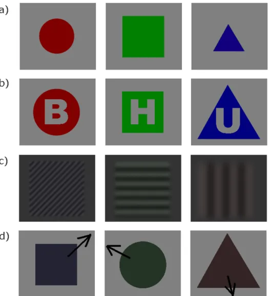
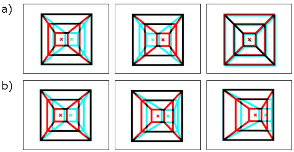
Figure 1. Examples of stimuli. First column shows stimuli with all three target attributes present, second and third columns with three non-target attributes.
a) Stimuli for experiment 3RedA
b) Stimuli for experiments 3RedB and 3RedC c) Stimuli for experiments 3RedD and 3RedDSat d) Stimuli for experiment 3RedE
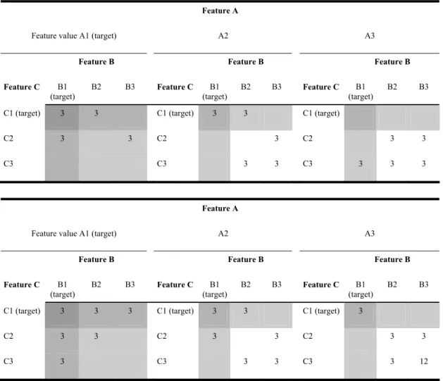
Table I. Stimulus distribution for one block for three target attributes, for 3redA (top) and all subsequent experiments (bottom). Panels, rows and columns show the different attribute values. White fields are non targets, light gray fields are stimuli with one target attribute, medium gray fields are stimuli with two target attributes, and the dark gray field represents a stimulus with all three target attributes present.
Feature A
Feature value A1 (target) A2 A3
Feature B Feature B Feature B
Feature C B1 (target) B2 B3 Feature C B1 (target) B2 B3 Feature C B1 (target) B2 B3
C1 (target) 3 3 C1 (target) 3 3 C1 (target)
C2 3 3 C2 3 C2 3 3
C3 C3 3 3 C3 3 3 3
Feature A
Feature value A1 (target) A2 A3
Feature B Feature B Feature B
Feature C B1
(target) B2 B3 Feature C (target)B1 B2 B3 Feature C (target) B1 B2 B3 C1 (target) 3 3 3 C1 (target) 3 3 C1 (target) 3
C2 3 3 C2 3 3 C2 3 3
Results
Participants performed very well on the task, with an average of 0.1 % of misses (1 miss per 357 Go-trials per participant) and 1.3 % of false alarms (9.25 false alarms per 357 NoGo-trials per participant). They maintained a mean response time (RT) of 373 ms with a standard deviation (std) of 91 ms across conditions.
Response times varied greatly across conditions and participants. Participants mean response times varied between 400 ms (std: 90 ms) and 314 ms (std: 85 ms). Mean response times in conditions where only one target attribute was presented (colour only: c, form only: f, or size only: s) were 392, 382, and 485 ms respectively (std: 79, 78, and 107 ms respectively). In double-redundant conditions, i.e. conditions with two target attributes present (colour and form: cf, colour and size: cs, or form and size: fs), mean RTs were 319, 342, and 373 ms respectively (std: 46, 55, and 78 respectively). In the triple-redundant condition (all three target attributes present, cfs) the mean RT was 322 ms (std: 64 ms). Note that the variation between participant means is almost half as large as the difference in means of the slowest (s) and fastest (cfs) conditions.
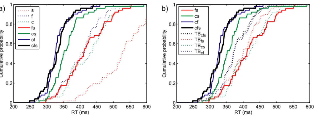
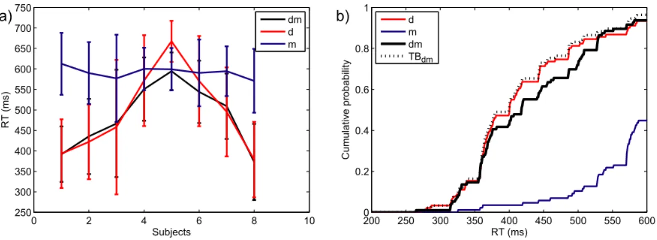
Figure 2 a) shows the cumulative response time distributions of one representative participant, for all three single-target conditions, as well as for all three conditions where two target attributes were presented simultaneously, and the triple redundant condition. The probability of responding at time t or faster is plotted as a function of time. All participants were significantly faster in the
double redundant conditions cf and cs than in their constituent single target conditions (mean value of the Anderson-Darling test: cf vs. c: AD = 20.08, cf vs. f: AD = 16.69, cs vs. c: AD = 10.44, cs vs. s: AD = 26.53; the critical value of the AD test being 2.49 for a type I error rate of .05). All participants also responded significantly faster to form and size (fs) than to size alone (mean AD = 18.27). However, only participant 2 was significantly faster in condition fs than when only form was present as a target attribute (AD = 3.02). In the triple redundant condition, all participants were significantly faster than in the double redundant condition fs (mean AD = 12.44), three of four participants were faster than in condition cs (mean AD = 6.02), and none of the participants was faster than in condition cf (mean AD = 1.11).
Figure 2 b) shows the cumulative response time distributions for a representative participant of the three double redundant conditions as well as the triple redundant condition. Additionally it shows the Townsend Bound for each of these conditions. The Townsend Bound gives the upper limit of race model performance, based on the RT distributions of this participant in the single target conditions. All four participants respond significantly faster than the Townsend Bound in the triple redundant condition (mean AD = 6.73), as well as in the double redundant conditions cf (mean AD = 9.00) and cs (mean AD = 7.25). However, in the condition fs participants did not pass the Townsend Bound (mean AD = 1.17).
Figure 2. Experiment 3RedA: Performance of participant 3.
a) RT distributions for single, double and triple redundant conditions. Dotted coloured lines are the cumulative distributions for single-target conditions, full coloured lines for double redundant conditions, black for the triple redundant condition.
b) Townsend Bounds for triple and double redundant conditions. Coloured lines are double redundant RT distributions, the black line the triple redundant condition. Dotted lines of the same colour are the Townsend Bounds for the respective conditions.
200 250 300 350 400 450 500 550 600 0 0.2 0.4 0.6 0.8 1 RT (ms) Cumulative probability s f c fs cs cf cfs 200 250 300 350 400 450 500 550 600 0 0.2 0.4 0.6 0.8 1 RT (ms) Cumulative probability fs cs cf cfs TBcfs TBfs TBcs TBcf a) b)
As was to be expected from previous studies on redundancy gain, we managed to replicate findings of double redundancy gain that surpass the performance predicted by race models. However, we have not found evidence of a triple redundancy gain.
There are several patterns to be observed in these results. First, the attribute size is significantly slower than either colour or form for all participants. Second, participants perform equally well when both target attributes form and size are present than when colour only or form only are present. Third, performance on triple redundant trials and performance on trials with colour and form present does not differ significantly for any participant.
We therefore conclude that even though the Townsend Bound was violated for all participants in the triple redundant condition, these results cannot be evidence for a possible triple redundancy gain, nor for coactivation as an explanation of such a gain. Since the RT distributions for conditions cfs and cf do not differ in speed, all the gain in the triple redundant condition can be attributed to the presence of colour and form as target attributes. The presence of size does not seem to contribute to an additional gain.
In order to be able to observe a triple redundancy gain, it might be important that all target attributes have the opportunity to contribute equally to such a gain. If the recognition of one attribute is already much slower than the other two, this attribute can only contribute minimally, if at all, since the
advantage of its presence is negligible compared to the presence of two easily recognisable attributes.
This leads to the question why response times for size were slower than for colour or form. The most noticeable difference is that colour and form are absolute values, whereas size is a relative measure. The value of “large” or “small” only takes on meaning in relation to a reference, whereas “red” or “square” can be defined without a reference. In all further experiments we therefore chose only to investigate absolute target attributes.
We hypothesized that single target response time distributions need to be as close as possible to the same speed to be able to observe maximal redundancy gain. If one target attribute is processed noticeably slower than the other two, this attribute cannot contribute sufficiently to triple redundancy gain. There are a number of underlying processes involved in the processing of a visual stimulus (e.g. detection, identification, decision, and motor response). The speed of each of these processes, depending on the speed of the attribute to be processed, cannot be estimated, nor can their mutual independence be established. Therefore it is not possible to estimate a priori the processing speed of any given visual attribute. The most practicable solution to this problem is to test empirically a large number of different attributes until finding a set of three attributes which are processed at approximately the same speed. In this case, we would predict that triple redundancy gain is larger than double redundancy gain.
Further research: General method
The procedure and design of all further pilot experiments, designed to find an appropriate set of target attributes, stayed essentially the same as for the first experiment. Stimulus size was maintained at 3°VA (degree of visual angle). However, the stimulus attributes change for each experiment. Also, all further experiments use a different distribution of stimuli than the one used in 3RedA (and as a result of this, a different number of blocks per experiment and trials per block). Finally, presentation times of stimuli, as well as the time frame for participants to respond, were considerably shortened.
For all further experiments we used the stimulus distribution illustrated in Table I (bottom). This was done for two reasons. First, we felt it was necessary to include all possible combinations of attributes. In the distribution proposed by Mordkoff and Yantis (1991), target attributes were only combined with other target attributes or one of the two possible non-target values. The other non-target value was automatically associated with a non-target. In the case of the stimulus distribution used in this experiment, this meant that certain target attributes (such as the colour red) were never combined with one of the two possible non-target values of one of the other two stimulus dimensions (i.e. form or size). In order to reduce the impact of the identity of the non-target attribute, we felt that it was important for the non-target attribute(s) on single and double redundant targets not to be predictable. Secondly, by combining all possible attributes, we had the means of evaluating the impact of certain contingencies mentioned by Mordkoff
and Yantis (1991, 1993), thereby calculating the contribution of crosstalk to redundancy gain. There are now two types of stimuli per double redundant condition, one with each type of non-target attribute, therefore we can compare RTs in the double redundant conditions depending on non-target type (see chapter two for details on this).
However, this choice made finding a distribution of stimuli with three different attributes that satisfied the criteria formulated by Mordkoff and Yantis (1991) much harder. In the end, in order to keep 50% of targets, with more combinations of target and non-target attributes, and avoid facilitatory contingencies, we accepted certain inhibitory contingencies. But, as mentioned above, these contingencies would potentially slow down recognition of redundant targets, and also, we had the means to evaluate their impact. Therefore this choice of a stimulus distribution is conservative with respect to our goal of attributing redundancy gain to coactivation, and can be considered valid.
As a result of the new distribution, subsequent experiments consisted of 16 blocks per experimental session, with 60 trials per block, for a total of 960 trials. Presentation time of the fixation point preceding the stimulus was shortened to 494 ms, stimulus presentation itself was shortened to approximately 750 ms (this varied slightly between experiments, depending on the stimulus). The time limit for participants to respond to a stimulus was set at 750 ms after stimulus onset, and the feedback slide was presented for 753 ms only.
Practice effects
It is conceivable that practice effects (Newell & Rosenbloom, 1981) could have an effect on the observed redundancy gain. Either response times on single target trials might improve, thereby leaving less room for redundancy gain, or treatment on single target trials might stay the same while participants become experts on recognition of redundant trials, i.e. experts at recognising certain
combinations of attributes. Since the task was fairly easy (low error rates in
experiment 3RedA), we judged that practice effects if any would be visible after the completion of two sessions of approximately 45 minutes each. This hypothesis was tested in the following experiment.
3RedB : Colour, form and letter
Method. Three female undergrads from the Université de Montréal, with
normal or corrected-to-normal vision, were compensated with 8$ for their participation. For the reasons mentioned above, the target attribute size was replaced by the attribute letter. Stimuli were 3°VA in size, and varied in colour (red, green, or blue) and form (circle, square, or triangle). Each shape contained a cut out letter (either an H, a U or a B) of 2.7 degrees of visual angle (see Figure 1 b). Target attributes were red, circle, and the letter B. The letter B as a target was chosen because it shares attributes with both non-target letters. This experiment consisted of two experimental sessions, each with 960 trials, which were completed over two consecutive days by three subjects. This was done to test for potential effects of training that might influence the amount of redundancy gain
observed. All other design and procedure details remain the same as mentioned above.
Results. Error rates were as low as expected, with 0.07 % of misses (0.33
misses per 480 Go-trials) and 0.69 % of false alarms (3.33 per 480 NoGo-trials) in session one, and 0.07 % of misses (0.33 per 480 trials) and 1.11 % of false alarms (5.33 per 480 trials) in session two. Neither the number of misses (t(4) = 0, p = 1) nor the number of false alarms (t(4) = -0.59, p = 0.59) differed significantly between sessions.
An analysis of variance of mean response times by condition and session reveals that all participants respond significantly faster in session two than in session one (F(1,28) = 12.22, p < 0.002), and faster in the triple redundant condition than in the double or non-redundant conditions (F(6,28) = 3.26, p < 0.015). However, there is no interaction between condition and session (F(6,28) = 0.2, p = 0.97). We conclude that although practice does have an effect on response times, performance increases equally independent of the degree of redundancy. Therefore there is no effect of practice on the amount of redundancy gain between conditions. All subsequent experiments will contain only one experimental session of the above-mentioned length.
Analogous to other experiments, analysis of redundancy gains is done only on session one. As expected, participants mean response times varied a lot (participant 1: 393 ms (std 68); participant 2: 478 ms (std 155); participant 3: 362 ms (std 69)), as did response times between conditions. Mean response times in
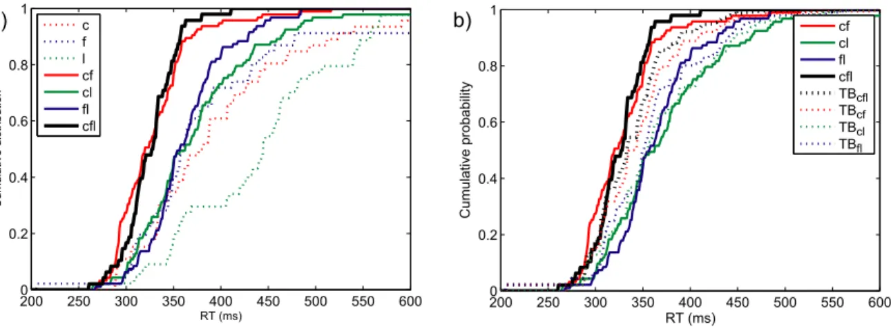
conditions where only one target attribute was presented (colour only: c, form only: f, or letter only: l) were 417, 482, and 459 ms respectively (std: 98, 132, and 163 ms respectively. In double-redundant conditions, i.e. conditions with two target attributes present (colour and form: cf, colour and letter: cl, or form and letter: fl), mean RTs were 389, 383, and 423 ms respectively (std: 85, 93, and 122 respectively). In the triple-redundant condition (all three target attributes present, cfl) the mean RT was 358 ms (std: 84 ms).
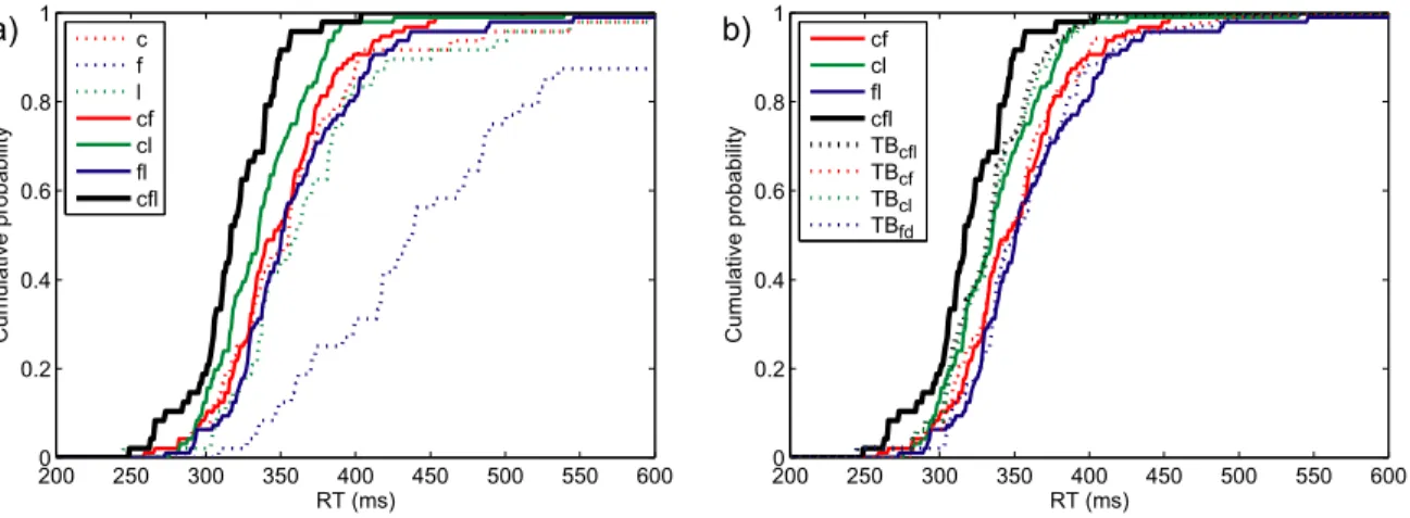
Figure 3 a) shows the cumulative response time distributions of one representative participant, for all three single-target conditions, as well as for all three conditions where two target attributes were presented simultaneously, and the triple redundant condition. The probability of responding at time t or faster is plotted as a function of time. Only one participant showed a significant double redundancy gain for all three double redundant conditions over all single target conditions (value of the Anderson-Darling test between 28.42 and 6.96; the critical value of the AD test being 2.49 for a type I error rate of .05). For the other two participants, the combination of form and letter was not significantly faster than letter only, the faster of the two single target conditions (mean AD = 1.01). The combination of colour and letter was significantly faster than colour, the faster of the two single-target conditions, for one participant, but not for the other (AD = 2.60 and AD = 0.66 respectively). In the triple redundant condition, all participants were significantly faster than in the double redundant condition fl (mean AD = 14.74), and two out of three participants were faster than in condition cl (mean AD = 4.26) and in condition cf (mean AD = 8.16).
Figure 3. Experiment 3RedB: Performance of participant 3.
a) RT distributions for single, double and triple redundant conditions. Dotted coloured lines are the cumulative distributions for single-target conditions, full coloured lines for double redundant conditions, black for the triple redundant condition.
b) Townsend Bounds for triple and double redundant conditions. Coloured lines are double redundant RT distributions, the black line the triple redundant condition. Dotted lines of the same colour are the Townsend Bounds for the respective conditions.
200 250 300 350 400 450 500 550 600 0 0.2 0.4 0.6 0.8 1 RT (ms) Cumulative pr obability c f l cf cl fl cfl 2000 250 300 350 400 450 500 550 600 0.2 0.4 0.6 0.8 1 RT (ms) Cumulative pr obability cf cl fl cfl TBcfl TBcf TBcl TBfd a) b)
Figure 3 b) shows the cumulative response time distributions for a representative participant of the three double redundant conditions as well as the triple redundant condition. Additionally it shows the Townsend Bound for each of these conditions. The Townsend Bound gives the upper limit of race model performance, based on the RT distributions of this participant in the single target conditions. All three participants responded significantly faster than the Townsend Bound in the triple redundant condition (mean AD = 3.02). However, in all three double redundant conditions, only one participant was significantly faster than the corresponding Townsend Bound (cf: AD = 4.90; cl: AD = 6.62; fl: AD = 3.48).
Not all participants showed a significant redundancy gain in the double redundant conditions, let alone a gain large enough to overcome the Townsend Bound, and thus provide evidence against race models. Therefore we conclude that the gain observed in the triple redundant condition is again due to the interaction of two target attributes, without contribution of a third. This is supported by the fact that for all participants, the attribute form is processed slower than the other two attributes. Notably, when comparing the response time distributions of the double redundant conditions cf and fl to the distributions for single attributes, cf and c are practically overlapping (see Figure 3 a), as are fl and l, whereas form is visibly slower. Even at a double redundant level, one can conclude that form hardly contributes to an increase in performance. Since in experiment 3RedA form and colour were processed at approximately the same speed, we conclude that the relative decrease of performance for form is related to the addition of the attribute letter. This might be because letter and form are essentially two variations of the
same attribute, or because the attribute letter is more familiar (participants are exposed to letters innumerable times in everyday life), and might therefore be processed more easily (Wang, Cavanagh & Green, 1994).
Effects of masking
In an attempt to counteract the processing advantage the attribute letter has over form, stimuli were masked after a brief delay in the subsequent experiment. We hypothesised that since “reading” of a letter happens at a later stage in the processing pathway than identification of form (Kandel et al., 2000), a very brief exposure of the stimulus would force participants to process form and letter similarly, and thus equalise response time distributions of the two attributes. Another reason for masking was to avoid benefit from a visual imprint or afterimage left by the stimulus.
3RedC: Masked
Method. Six undergrads (3 male) from the Université de Montréal, with
normal or corrected-to-normal vision, were compensated with 8$ for their participation. Stimuli remained the same as for 3RedB (Figure 1b), except that the target colour was switched to green because this colour is less salient than red, in an attempt to render colour recognition slightly more difficult. The target form was also switched from circle to square, because a square shares attributes of each of the other two attributes, analogous to the target letter B, which shares characteristics of both non-target letters. Masks were constituted of four quadrants
from four randomly selected stimuli. Stimuli were presented for 75 ms, followed by a mask for 925 ms. All other methodological details are the same as mentioned above.
Results. Error rates were still low, although a little higher than in previous
experiments, with 2.08 % of misses (10 misses per 480 Go-trials) and 4.03 % of false alarms (19.3 per 480 NoGo-trials). Mean response times varied between 364 ms and 519 ms across participants.
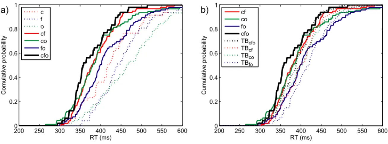
Mean response times over all participants in conditions where only one target attribute was presented (colour only: c, form only: f, or letter only: l) were 458, 476, and 485 ms respectively (std: 134, 149, and 125 ms respectively). Compared to experiment 3RedB, the difference between the mean RT of the fastest and slowest single-target condition has more than halved (3RedB: 65 ms; 3RedC: 27 ms). Processing speed of the three attributes seems to be more similar. The double-redundant conditions also had very similar mean RTs (cf: 409 ms (std 119 ms); cl: 420 ms (std 105 ms); fl: 419 ms (std 114 ms)). In the triple-redundant condition the mean RT was 384 ms (std: 100 ms).
Figure 4 a) shows the cumulative response time distributions of one representative participant, for all three single-target conditions, as well as for all three conditions where two target attributes were presented simultaneously, and the triple redundant condition. The probability of responding at time t or faster is plotted as a function of time. Five participants responded significantly faster in double redundant condition cf than in condition c (mean AD = 7.50; the critical
value of the AD test being 2.49 for a type I error rate of .05) and four participants faster than condition f (mean AD = 10.38). Two and four participants responded faster in condition cl than in conditions c (mean AD = 6.82) and l (mean AD = 11.27). Five participants responded significantly faster in condition fl than in f (mean AD = 5.04) or l (mean AD = 11.52). In the triple redundant condition, three, five and four participants responded significantly faster than in the conditions cf (mean AD = 5.10), cl (mean AD = 7.27), or fl (mean AD = 9.05) respectively.
Figure 4 b) shows the cumulative response time distributions for a representative participant of the three double redundant conditions as well as the triple redundant condition. Additionally it shows the Townsend Bound for each of these conditions. The Townsend Bound gives the upper limit of race model performance, based on the RT distributions of this participant in the single target conditions. Only one participant, in condition cf, performed significantly faster than the Townsend Bound for that condition (AD = 4.85). All other response time distributions in double or triple redundant conditions were not significantly different from their respective Townsend Bounds.
Figure 4. Experiment 3RedC: Performance of participant 3.
a) RT distributions for single, double and triple redundant conditions. Dotted coloured lines are the cumulative distributions for single-target conditions, full coloured lines for double redundant conditions, black for the triple redundant condition.
b) Townsend Bounds for triple and double redundant conditions. Coloured lines are double redundant RT distributions, the black line the triple redundant condition. Dotted lines of the same colour are the Townsend Bounds for the respective conditions.
2000 250 300 350 400 450 500 550 600 0.2 0.4 0.6 0.8 1 RT (ms) Cumulative probability cf cl fl cfl TBcfl TBcf TBcl TBfl 2000 250 300 350 400 450 500 550 600 0.2 0.4 0.6 0.8 1 RT (ms) Cum ulativ e dis tribution c f l cf cl fl cfl a) b)
The total absence of evidence in favour of coactivation models in this experiment is rather surprising, especially so since conditions for observing maximal redundancy gain were better here than in previous experiments (given our assumption is correct in that redundancy gain is maximal if single targets are processed as close as possible to the same speed). The variance between processing speed of single targets is smaller in this experiment than in previous ones, and processing speed for letter is similar to that of form – for some participants, form is even faster than letter.
We hypothesize that the disappearance of evidence against race models might be related to the masking of stimuli. To test for a causal relation between masking and the amount of redundancy gain observed, an experiment which balances masked and non-masked trials is conceived.
2RedM&M: Masked / Unmasked
Method. To test the effect of a mask on redundancy gain, response times of
four undergrads (1 female) from the Université de Montréal, with normal or corrected-to-normal vision, were measured in a Go-NoGo paradigm, with stimuli defined by two attributes, colour and form. Target stimuli were green and/ or square. Masks consisted of quadrants from four randomly selected stimuli. The experiment consisted of two experimental sessions, one in which stimuli were masked, the other in which they were unmasked, counterbalanced across participants. Sessions consisted of 576 trials each, half of which were non-target trials. Stimuli were presented for 1000 ms in the unmasked condition and for 75
ms, followed by a mask of 925 ms, in the masked condition. Analogous to the 3Red experiments, stimuli were preceded by a fixation point and followed by a feedback slide.
Results. An analysis of variance of mean response times by subject,
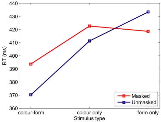
stimulus type (redundant, colour only or form only) and session (masked or unmasked) reveals that although participants respond significantly faster to redundant than to non-redundant stimuli (F(2,8) = 10.43, p < 0.006), response times do not differ whether stimuli are unmasked or masked (F(1,8) = 0.65, p = 0.44), and there is no interaction between stimulus type and session (F(2,8) = 1.84, p = 0.22) (see Figure 5 for a plot of mean response times by session and stimulus type). We conclude that masking does not have an effect on response times in general, or on the amount of redundancy gain between conditions.
Figure 5. 2RedM&M: effect of condition and masking on response times. Conditions are plotted on the x-axis. Mean response times when stimuli were masked are plotted in red, unmasked in blue.
colour-form colour only form only
360 370 380 390 400 410 420 430 440 Stimulus type RT (ms) Masked Unmasked
In order to find an answer to two major problems in the previous experiments, we decided to look at the structure of the visual processing pathway in the brain. First, this might help us find an appropriate combination of three target attributes. Up to now, one attribute was always considerably slower than the other two, and therefore affected the triple redundancy gain. Second, we needed to explain the mixture of our results: for some combinations (pairs or set of three) of attributes we find redundancy gain significantly faster than the Townsend Bound, for others no redundancy gain, or gain but not above the Townsend Bound. This could also be related to the structure of visual processing areas.
Note that we do not wish to establish a causal relation between the structure of the visual system and our results. We merely use it as an indication to point us in the right direction. The main foundation for the conception of further experiments remains empirical data.
Early processing stages
Visual processing is organised in a hierarchical fashion, going from the analysis of single neuron responses to more and more complex units of information (Maunsell & Newsome, 1987). The primary visual processing area V1 is the first area of visual processing to receive input from both eyes, both from the Magnocellular and Parvocellular pathway (Hubel & Wiesel, 1979; Hubel, 1988). V1 is selective to orientation and spatial frequency information, which is used to define contours, one of the most basic features to be extracted from visual input (Hubel & Wiesel, 1962, 1979). Contours are what is essentially used in form
recognition, which means that form recognition can happen at a processing stage as early as V1. V1 is also selective to colour (Hubel, 1988; Livingstone & Hubel, 1987).
Colour and form seem to be the most reliable attributes across experiments (they are processed at roughly the same speed and produce redundancy gain fairly reliably faster than the Townsend Bound). If we break down form into its two components, spatial frequency and orientation, we get a set of three attributes which are all processed at a very early level in visual processing, and all in the same area, namely in V1. Since we know that colour and form are processed at roughly the same speed, we hypothesize that these three attributes will be as well.
3RedD : colour, orientation, frequency
Method. To test this hypothesis, four undergrads (1 male) from the
Université de Montréal, with normal or corrected-to-normal vision, participated in an experiment similar to those described above, with stimuli being defined by three attributes: colour, spatial frequency of bars and orientation of bars. Stimuli consisted of squares (size: 3°VA) filled with a sinusoidal gratings alternating between colour and gray of different cycle length and orientation. Luminance of stimuli was reduced to 20%, and saturation to 50%. Stimuli were presented in front of a gray background with luminance reduced to 20%. This was done to slow down the recognition of target attributes, in particular colour, thereby leaving more room for improvement due to redundancy. Also, the attribute spatial frequency is again a relative instead of an absolute attribute. Therefore the disadvantage to