HAL Id: hal-01860250
https://hal.archives-ouvertes.fr/hal-01860250
Submitted on 23 Aug 2018
HAL is a multi-disciplinary open access
archive for the deposit and dissemination of
sci-entific research documents, whether they are
pub-lished or not. The documents may come from
teaching and research institutions in France or
L’archive ouverte pluridisciplinaire HAL, est
destinée au dépôt et à la diffusion de documents
scientifiques de niveau recherche, publiés ou non,
émanant des établissements d’enseignement et de
recherche français ou étrangers, des laboratoires
Kinematic Spline Curves: A temporal invariant
descriptor for fast action recognition
Enjie Ghorbel, Rémi Boutteau, Jacques Boonaert, Xavier Savatier, Stéphane
Lecoeuche
To cite this version:
Enjie Ghorbel, Rémi Boutteau, Jacques Boonaert, Xavier Savatier, Stéphane Lecoeuche. Kinematic
Spline Curves: A temporal invariant descriptor for fast action recognition. Image and Vision
Com-puting, Elsevier, 2018, 77, pp.60-71. �10.1016/j.imavis.2018.06.004�. �hal-01860250�
Kinematic Spline Curves: A temporal invariant descriptor
for fast action recognition
Enjie Ghorbela,b,∗, R´emi Boutteaub, Jacques Boonaerta, Xavier Savatierb, St´ephane Lecoeuchea
aIMT Lille Douai, Univ. Lille, Unit de Recherche Informatique et Automatique, F-59000 Lille, France bNormandie Univ, UNIROUEN, ESIGELEC, IRSEEM, 76000 Rouen, France
Abstract
Over the last few decades, action recognition applications have attracted the growing interest of researchers, especially with the advent of RGB-D cameras. These applica-tions increasingly require fast processing. Therefore, it becomes important to include the computational latency in the evaluation criteria.
In this paper, we propose a novel human action descriptor based on skeleton data provided by RGB-D cameras for fast action recognition. The descriptor is built by in-terpolating the kinematics of skeleton joints (position, velocity and acceleration) using a cubic spline algorithm. A skeleton normalization is done to alleviate anthropomet-ric variability. To ensure rate invariance which is one of the most challenging issue in action recognition, a novel temporal normalization algorithm called Time Variable Replacement (TVR) is proposed. It is a change of variable of time by a variable that we call Normalized Action Time (NAT) varying in a fixed range and making the de-scriptors less sensitive to execution rate variability. To map time with NAT, increasing functions (called Time Variable Replacement Function (TVRF)) are used. Two dif-ferent Time Variable Replacement Functions (TVRF) are proposed in this paper: the Normalized Accumulated kinetic Energy (NAE) of the skeleton and the Normalized Pose Motion Signal Energy (NPMSE) of the skeleton. The action recognition is car-ried out using a linear Support Vector Machine (SVM). Experimental results on five challenging benchmarks show the effectiveness of our approach in terms of
recogni-∗Corresponding author
tion accuracy and computational latency.
Keywords: RBG-D cameras, action recognition, low computational latency, temporal normalization
1. Introduction
Human action recognition has represented an active field of research over the last decades. Indeed, it has become important due to its wide range of applications. As ex-ample, it could be cited video surveillance, Human Machine Interaction (HMI), gam-ing, home automation and e-health.
5
The first generation of approaches dealing with human action recognition was gen-erally based on Red Green Blue (RGB) videos. Many reviews of these methods can be found in the literature [1, 2]. However, RGB videos present some major disadvan-tages such as the sensitivity to illumination changes, occlusions, viewpoint changes and background extraction. To overcome these limitations, new acquisition systems have
10
recently been proposed to give additional information about the observed scene: Red Green Blue-Depth (RGB-D) cameras. Depth images have simplified and sped up the extraction of human skeletons via integrated libraries such as OpenNI and KinectSDK (around 45ms for skeleton extraction per frame according to [3]), which was a very difficult task with the use of RGB images. Other acquisition systems such as motion
15
capture systems provide more accurate skeleton sequences but remain unadapted due to their high cost and their non-portability.
In [4], it has been demonstrated that depth-based methods are generally more ac-curate than skeleton-based methods since depth modality is more robust to noise and occlusions. However, skeleton-based descriptors are faster to compute because of their
20
lower dimension and are therefore more suited for applications requiring a fast recog-nition.
Many recent papers have proposed RGB-D-based descriptors for human action recognition, showing their high accuracy of recognition in various datasets [5, 6, 7, 8, 9, 10, 11]. Nevertheless, a central challenge is often omitted in these earlier papers:
25
does not work in real-time, its usability in real-life applications remains limited. Thus, the performance of motion descriptors can be viewed as a trade-off between accuracy of recognition and low latency as mentioned in [12], where latency is defined as the sum of computational latency (the time necessary for computation) and observational
30
latency (the time of observation required to make a good decision). In this paper, we will focus mainly on computational latency because the actions are assumed to have already been segmented. Indeed, many off-line applications still require a quick recog-nition such as medical rehabilitation, gaming, coaching, etc.
Based on these observations, we propose a new skeleton-based human action
de-35
scriptor called Kinematic Spline Curves (KSC) which operates with low computational latency and with acceptable accuracy compared with recent state-of-the-art methods. To build this descriptor, a Skeleton Normalization (SN) is first carried out to overcome the anthropometric variation. Then, kinematic features including joint position, joint velocity and joint acceleration are calculated from the normalized skeleton data.
40
After this step, a Temporal Normalization (TN) is carried out in order to reduce the effect of execution rate variability. The TN introduced in this paper is called Time Variable Replacement (TVR). It is based on a change of variables of time by a variable called Normalized Action Time (NAT). Thus, this variable is invariant to execution rate and varies in a fixed range whatever the length of the action is. Functions that can be
45
used to do this change of variables are called Time Variable Replacement Functions (TVRF). In this article, Two TVRF are introduced, namely, the Normalized Accumu-lated kinetic Energy (NAE) of the skeleton and the Normalized Pose Motion Signal Energy (NPMSE).
This step is a novel, fast and simple way to make actions with different execution
50
rate comparable, without the loss of the temporal information. Finally, features are interpolated via a cubic spline interpolation and are uniformly sampled in order to obtain vectors with the same size.
To achieve a fair comparison of our descriptor with other approaches in terms of accuracy and computational latency, we report the accuracy of recognition and the
55
execution time per descriptor on various challenging benchmarks. Available algorithms of recent state-of-the-art methods are tested with the same parameters and settings on
four datasets: MSRAction3D dataset [5] UTKinect dataset [13], MSRC12 dataset [14] and Multiview3D Action dataset [15]. Our descriptor is also tested on a large-scale dataset NTU RGB+D dataset [16].
60
Based on our previous work [17], the paper presents a complete action recognition method including novelties such as: 1) The generalization and the extension of a fast and simple novel Temporal Normalization (TN) method called Time Variable Replace-ment (TVR) in order to avoid the execution rate variability. 2) The detailed analysis of the different component influence (kinetic values, temporal normalization, spatial
65
normalization, etc). 3) A larger experimentation by including three other challenging benchmarks (MSRC-12, Multiview3D and NTU RGB+D datasets).
This article follows this scheme: in Section 2, an overview of related methods is given. Section 3 presents the concept of cubic spline interpolation and Section 4 presents the methodology used to build our descriptor. In Section 5, the experiments
70
and the results are discussed. Finally, Section 6 summarizes this paper and includes some ideas for future work.
2. Related work
In a recent survey [18], action recognition methods have been categorized accord-ing to the nature of the used representation: learned representations and hand-crafted
75
representations.
Hand-crafted methods are the most common approaches used in the literature [6, 8, 19]. They are based on the classical schema of action recognition, where low-level features are first extracted, then the final descriptor is modeled using low level features and finally a classifier is used to train a classification model such as Support Vector
80
Machine (SVM) or k Nearest Neighbors (kNN).
With the recent advances in deep learning, learning-based representations have been proposed. Instead of selecting specific features, this category of methods learn itself the appropriate ones as in [20, 21, 22, 23, 24]. These methods are very interest-ing and efficient. However, they require an important amount of data, as well as an
85
In this paper, we focus on hand-crafted methods, since we are interested in recog-nizing actions using small scale datasets.
The RGB-D-based human action descriptors are commonly divided into two cate-gories, namely depth-based descriptors and skeleton-based descriptors.
90
2.1. Depth-based descriptors
The first tendency was to adapt motion descriptors, initially developed for RGB or gray-level images, to depth images. For example, we can cite the work of [25] where the Spatio-Temporal Interest Points detector (STIP) [26] and the cuboid de-scriptor [27] were adapted to depth images. They called them respectively the
Depth-95
Spatio-Temporal Interest Points (DSTIP) and the Depth-Similarity Cuboid Features (DSCF).
Other examples can be mentioned such as the extension of Histogram of Oriented Gradient (HOG) [28] to the HOG3D [29] and also its extension to HOG2 [6]. However, some researchers rapidly pointed out the limitations of these adapted methods
justify-100
ing their claims by the fact that depth modality has different properties and a different structure from color modality [7, 9].
Because of the popularity of the Bag-Of-Words approach and its variants in the field of RGB-based action recognition [30, 31], many attempts have been made to extend this kind of methods to depth modality [32, 33, 34].
105
Less conventional depth-based descriptors were also proposed [7, 35, 36, 9]. One of the most efficient representations that we can cite is the 4D normals. This origi-nal idea was introduced in the work of [7] where the motion of the human body was considered as a hyper-surface of R4(three dimensions for the spatial components and one dimension for the temporal component). In differential geometry, one of the
well-110
known ways to characterize a hyper-surface is to find its normals. Thus, Oreifej and Liu chose these features and built the descriptors by quantifying a 4D histogram of normals using polychrons (a 4D extension of simple polygons [37]).
Many authors were inspired by this relevant representation, but changed the quan-tization step (because of the neighboring information loss with the use of HON4D).
115
the same time, Yang et al. [9] used the same representation by learning a sparse dictio-nary and then by coding each action as a word of the learned dictiodictio-nary. The obtained descriptor was called the Super Normal Vector (SNV). This new generation of features based on depth modality has shown its high accuracy compared to other
representa-120
tions. Notwithstanding this important advantage, they generally require considerable computation time as shown in Section 5.
2.2. Skeleton-based descriptors
One of the pioneer work proposed to build a 3D Histogram Oriented of Joints (HOJ) where the 3D position of joints is used [13]. Thus, each posture is represented by a
125
specific histogram. The evolution of these postures is included in a Hidden Markov Model (HMM) which is based on a bag of postures. These features are interesting but are very sensitive to anthropometric variability.
To reduce the effect of this body variation, new methods emerged, where the rel-ative position of joints were used instead of the absolute position as in [38]. These
130
authors [38] proposed the use of the spatial and temporal distances between joints as features. In [39, 40], the main idea is to calculate a similarity shape measure between joint trajectories. To realize that, these curves are reparametrized using the Square-Root Velocity Function (SRVF), leading to a representation in a Riemannian manifold. Recently, new skeleton-based descriptors have been proposed, inspired by earlier
135
bio-mechanical studies [41] where the skeleton was a very commonly-used represen-tation. Our work is principally inspired by these descriptors more particularly by the two following papers.
On the one hand, Vemulapalli et al. [8, 42] proposed to define the rotations and translations between adjacent skeleton segments using transformation matrices of the
140
Special Euclidean group SE(3). Therefore, the obtained features represent a concate-nation of transformation matrices expressed in SEn(3), where n is equal to the number of segment connections. To switch from a discrete space to a continuous one and to represent descriptors as curves of the Lie group SEn(3), an interpolation is done on the points of SEn(3) after the transition to sen(3), the Lie algebra associated with
145
account some important physical measures such as velocity and acceleration.
On the other hand, Zanfir et al. [43] chose to use the kinematics of skeleton joints as features: joint positions, joint velocities and joint accelerations. To overcome anthro-pometric variability, a skeleton normalization is done. After that, joint velocities and
150
joint accelerations are computed using the information from joint positions. The three kinematic values are then concatenated in a single vector, where the importance of each kinematic value is weighted by optimized parameters. Using this kinematic-based de-scriptor, the action recognition is done using a kNN classifier (k Nearest-Neighbors). Even if this method has given good results according to the experimentation of [43],
155
the discontinuity of features can generate some limitations. Indeed, the non-uniformity of velocity during acquisition or the presence of noisy skeletons can negatively impact the results.
3. Cubic spline Interpolation: A review
As presented in Introduction, a cubic spline interpolation will be used to interpolate
160
kinematic features. We reject the idea of using approximation instead of interpolation because of the low number of frames (generally between 20 and 50 per action in well-known datasets) favoring an inaccurate approximation. This method is a well-well-known numerical method which connects coherently a set of N points (αk, yk))k∈J1,N Kwith α1 < α2 < ... < αk < ... < αN. The goal is to estimate the function f which
165
is assumed to be a continuous C1 piecewise function of N − 1 cubic third degree polynomials fkas described by equation (1).
f (t) = (fk(t)) f or αk < t < αk+1 (1) Each function fk is defined on the slice [αk, αk+ 1] (2). In order to respect the continuity of f , each fkis joined at αkby fk−1(the first derivative yk0 = yk+1−yk
xk+1−xk and
the second derivative yk00 = yk+10−yk0
xk+1−xk of yk are also assumed to be continuous). The 170
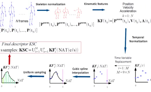
Figure 1: An overview of our approach: this figure describes the different steps to compute Kinematic Spline Curves (KSC). The first step represents the skeleton normalization which re-size skeleton to make it invariant to anthropometric variability. Based on the information of normalized joint positions, the joint velocities and joint accelerations are computed. Therefore, the three values are concatenated to obtain KF. To palliate execution rate variability, t is replaced by the NAT variable by using a Time Variable Replacement Function (TVRF). This step represents a novel temporal normalization method, referred as TVR. Then, each component KF is interpolated using a cubic spline algorithm in order to obtain M functions KFc. Finally, The uniform sampling of KFcallows us to build the final descriptor KSC.
(3). fk(α) = ak(α − αk)3+ bk(α − αk)2+ ck(α − αk) + dk (2) where ak= 1 (αk+1− αk)2 (−2yk+1− yk αk+1− αk + yk0 + yk+10) bk= 1 αk+1− αk(3 yk+1− yk αk+1− αk − 2yk0 − yk+10) ck= yk0 dk= yk (3)
degree polynomial which presents a maximum of one inflection point. Therefore, this kind of curve is at the same time realistic (in our case) and does not present undesired
175
oscillations. Furthermore, this algorithm presents low complexity, compared to other interesting interpolation techniques such as B-spline.
To carry out the cubic spline interpolation, a matlab toolbox implementing the algo-rithm proposed by [44] is directly used.
4. Kinematic Spline Curves (KSC)
180
In this section, we describe the different procedures allowing the calculation of the proposed human action descriptors KSC. Figure 1 illustrates these different processes. Each subsection details one of these steps.
4.1. Spatial Normalization (S.N.) via skeleton normalization
In this study, an action is represented by a skeleton sequence varying over time.
185
At each instant t, the skeleton is represented by the pose P(t), which is composed of n joints with the knowledge of their 3D position pj(t) = [xj(t), yj(t), zj(t)] with j ∈J1, nK .
P(t) = [p1(t), ..., pj(t), ..., pn(t)] (4) Thus, a skeleton sequence, which represents a specific action (segmented actions), can be seen as a multidimensional time series. As in the majority of bio-mechanical
190
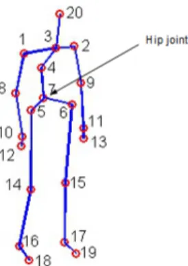
studies, the initial position of human hip joint is assumed to be the origin. This is why we subtract the hip joint coordinates phipfrom each joint coordinates. Figure 2 gives an example of skeleton and describes hip joint location.
P(t) = [p1(t) − phip, ..., pj(t) − phip, ..., pn(t) − phip] (5) Although we consider that the hip joint is the absolute origin, an important spatial variability continues to be present, mainly due to anthropometric variability. To
over-195
come this variability, we propose a skeleton normalization that is very similar to the normalization used in [43]. However, these latter chose to learn an average skeleton
Figure 2: Skeleton modality extracted using KinectSDK
for each dataset and then to constrain each skeleton of the dataset to have the same limb sizes. The problem is that in real-world applications, the average skeleton of a specific dataset cannot be representative. Thus, we propose the Euclidean normalization of
200
each segment length without imposing a specific length. Hence, we obtain skeletons with unitary segments. Each skeleton is normalized successively starting with the root (hip joint) and moving gradually to the connected segments. This approach preserves the shape of the skeleton and its performance will be discussed in the Section 5. Algo-rithm 1 describes the skeleton normalization used. All joint positions are normalized
205
except the hip joint position which is assumed to be the root and is therefore unchanged. pnorm
hip = phip.
We use the normalized skeleton sequence Pnormobtained after applying Algorithm 1 to phip to design our descriptor as depicted by equation (6). Since all joints are interconnected, we obtain a normalized position for each joint i, (pnormai , pnormb
i with
ai, bi∈J1, nK).
Pnorm= [pnorm1 , pnorm2 , ..., pnormn ] (6)
4.2. Kinematic Features (KF)
As in [43], we assume that human motion can be described by three important mechanical values: joint positions (normalized) Pnorm, joint velocities V and finally
Algorithm 1: Skeleton normalization at an instant t
Input : (pai(t), pbi(t))1≤i≤C represents the segment extremities ordered and
C represents the number of connections with aithe root extremity and bithe other extremity of the segment i
Output: (pnorm ai (t), p
norm
bi (t))1≤i≤C with ai, bi∈J1, nK 1 pnorma
1 (t) := pa1(t)(pa1(t) = phip(t) represents the position of the hip joint)
2 for i ← 1 to C (C:Number of segments) do 3 Si:= pai(t) − pbi(t) 4 s0i:= Si/distance(pai(t), pbi(t)) 5 pnormb i (t) := s 0 i+ p norm ai (t) 6 end
joint accelerations A. These values are concatenated to obtain what we call Kinematic Features (KF), noted KF in Equation (7).
KF(t) = [Pnorm(t), V(t), A(t))] (7) In this subsection, we describe how velocity (8) and acceleration (9) are numer-ically computed from the discrete data of joint positions as in [43]. In reality, the skeleton is composed of a skeleton sequence of N frames. k ∈ J1, N K denotes the
215
frame index and tkrepresents its associated instant.
V(tk) = Pnorm(tk+1) − Pnorm(tk−1) (8)
A(tk) = Pnorm(tk+2) + Pnorm(tk−2) − 2 × Pnorm(tk) (9) The dimension of the KF extracted from each frame is equal to M = 9 × n. We recall that n is the number of joints.
4.3. Time Variable Replacement (TVR) : a new approach for Temporal Normalization (TN)
220
Temporal variability is principally caused by execution rate variability (the tempo-ral differences that exist when a subject repeats a same action or when the different subject performs a same action), which implies changeable action duration and differ-ent distribution of motion. This means that actions are not performed in the same time slice as illustrated on the top panel of the Figure 3. Consequently, recognizing actions with features varying in different time slices proves to be difficult. For this reason, Temporal Normalization (T.N.) is needed to improve the efficiency of our method. We propose to interpolate the components of the features, according to a novel variable called Normalized Action Time (NAT), instead of time. This change of variable is done thanks to a function TVRF which places the actions in a space that is invariant to execution rate variability as shown in Figure 3. Therefore, the KF can be expressed as a variable depending on NAT which is rate-invariant (10).
KF(N AT ) = [Pnorm(N AT ), V(N AT ), A(N AT )] (10) The choice of the function TVFR is crucial for the good functioning of the normal-ization.
1) First, this function should have a physical meaning which makes features invari-ant to the execution rate variability.
2) Second, the used function should be increasing and have to realize a one-to-one
225
correspondence with time.
3) Finally, to compare actions with different temporal length, the latter function should vary in a fixed range independently from the length of the skeleton sequence as described by Figure 4.
In this way, let consider the T V RFinstance(instance represents the index of the
230
action instance) as an increasing one-to-one correspondence between the variable in-terval of time and a fixed inin-terval where NAT varies:
∀instance, T V RFinstance: [0, Ninstance] −→ [a, b] t 7−→ T V RFinstance(t) = N AT
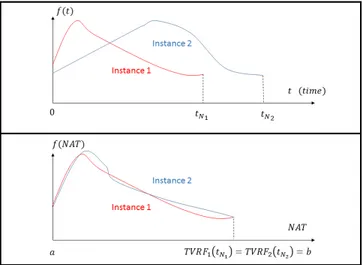
Figure 3: Example of the effect of temporal normalization on a joint component trajectory f (t). In this example, f (t) refers to the x-coordinates of a joint. We consider two instances of the same type of action (Instance1 and Instance2). Top: the trajectories are plotted as functions of time. We can observe that the time slices of the two trajectories are different ( tN16= tN2). Bottom: After the substitution of time by a NAT, we
can observe that the trajectories vary in the same range [a,b]. An important remark can also be made: the two trajectories representing the same action type are more similar.
a, b represent constant values such as [a, b] is the range where varies NAT and Ninstanceis the length of the skeleton sequence instance. This TVR algorithm is ex-pected to improve the accuracy of recognition of our method, since the time-variable
235
features are expressed in a same interval by replacing the time variable by a rate-invariant NAT variable. Thus, the good functioning of this approach is deeply related to the choice of NAT, and consequently to the choice of the TVRF. We present in this paper two different TVRF respecting the mentioned conditions: the Normalized Accu-mulated kinetic Energy (NAE) of the skeleton and the Normalized Pose Motion Signal
240
Energy (NPMSE).
4.3.1. Normalized Accumulated kinetic Energy of the skeleton (NAE) as a Time Re-placement Variable Function (TVRF)
The Normalized Accumulated kinetic Energy (NAE) of the skeleton is proposed as a Time Replacement Variable Function (TVRF). At an instant t and for each instant
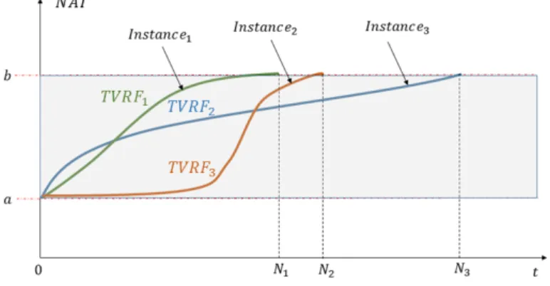
Figure 4: Let Instance1, Instance2and Instance3be three skeleton sequences with a temporal length
respectively equal to N1, N2and N3. This figure shows how the TVR allows the expression of different
instances with different temporal range in a same fixed range [a, b]
instance, NAE refers to the ratio N AE(t) between the kinetic energy Ekinetic acc (t) consumed by the human body until t and the total kinetic energy Ekinetic
total consumed by the human body on the whole skeleton sequence composed of N frames. Equation (11) describes this new term where E(t) represents the kinetic energy consumed by the human body at an instant t.
250 N AT = T V RFinst(t) = N AE(t) = E kinetic acc (t) Ekinetic total (11) Since the data structure is discrete. For each punctual instant tk, NAE is calcu-lated as follows in Equation (12). We recall that N represents the number of frames
contained in the skeleton sequence. N AT = T V RFinst(tk) = N AE(tk) = Ekinetic acc (tk) Ekinetic total = tk P c1=1 Ekinetic(c 1) N P c2=1 Ekinetic(c 2) (12)
Indeed, the NAE variable increases when the velocity of joints increases and conse-quently when the displacement quantity increases as well. If there is no motion, NAE
255
does not increase. We use NAE for two essential reasons. First, all actions must be expressed in the same space which is guaranteed by the normalization of the energy (varying between 0 and 1). Secondly, to perform a coherent interpolation, a growing variable is necessary. This is why accumulation is used.
Kinetic Energy Calculation: Instead of considering the skeleton as a body, it can
260
be assimilated to a set of n points where each one represents a skeleton joint. In many earlier papers [45, 46, 47], the kinetic energy of the human skeleton Ekinetic(t
k), at an instant tk, is expressed by the equation (13) where n represents the number of joints, mi and Vi, respectively, the mass and the velocity of the joint i. Since the skeleton joints are fictitious, we assume that they have a unitary mass (mi= 1, ∀i).
265 Ekinetic(tk) = n X i=1 1 2miV 2 i (tk) = n X i=1 1 2V 2 i (tk) (13) The NAE term N AE(tk) is calculated, thanks to the kinetic energy term Ekinetic(tk) (13) described in the previous paragraph following equation (11). After a change of variables, the KF can be expressed as a variable depending on NAE (10). Hence, Kinematic Features are expressed in the same range [0, 1] and become therefore less sensitive to execution rate variability.
270
4.3.2. Normalized Pose Motion Signal Energy (NPMSE) as a Time Variable Replace-ment Function (TVRF)
A second TVRF is proposed to replace the time variable called Normalized Pose Motion Signal Energy (NPMSE).
Before defining the notion of Pose Motion, we need to define the rest pose. The
275
rest pose represents the position of the spatially normalized skeleton when any gesture can be visually detected as in Figure 2.
To obtain this rest pose, a statistical model could be learnt using the training data. For the moment, since we are still working with temporally segmented data and since we know that all actions in the used datasets start with the rest pose, we can use the
280
first skeleton of the sequence to define the rest pose.
We define the Pose Motion Signal s(t) as the distance d between the current pose Pnorm(t) and the rest pose Pnorm(rest) (first pose in our experimental conditions) (14).
s(t) = d(Pnorm(t), Pnorm(rest)) (14) This used distance can be l2, l1, etc. More details about the nature of the distance
285
will be given in the experimental section. Since the available data has a discrete nature, the energy of the discrete signal s(tk) at an instant tk is calculated as follows (15). This term is called Pose Motion Signal Energy.
Esignal(tk) = k X i=1
|s(ti)|2 (15)
It is important to specify that in this paragraph the energy calculated is the signal energy and not the kinetic one, which are two different notions.
290
The Pose Motion Signal Energy is a growing term, thanks to the use of the sum in the energy calculation. However, to ensure that all the actions will be expressed in the same range, a normalization of this term has to be done. For an instance instance, the TVRF is therefore the Normalized Pose Motion Signal Energy (NPMSE) which is calculated by dividing the Pose Motion Signal Energy at an instant t by the Pose
295
Motion Signal Energy at the final instant of the sequence tf as described by equation (16).
N AT = T V RFinstance(t) = N P SM E(t) = E
signal(t)
Since the time data are discrete, the NPMSE at an instant tkis calculated as follows (17). N AT = T V RFinstance(tk) = N P M SE(tk) = E signal(tk) Esignal(t N) = Pk i=1|s(ti)|2 PN i=1|s(ti)|2 (17) Relation with key poses:The idea of using the distance between the current pose and
300
the rest pose provides from the fact that the more the poses are different from the rest state, the more they can discriminate actions. It is in a certain way related to the notion of key poses presented in many papers [48, 49, 50], where the key pose is defined as the extreme pose of an action. In [48], authors show that this kind of pose is sufficient to obtain interesting results. However, this kind of method does not
305
include the spatio-temporal aspect which is also important. For this reason, we propose this TVRF function which exploits the notion of keypose without removing the spatio-temporal aspect.
4.4. Cubic spline interpolation of Kinematic Features (KF)
Based on the continuous nature of human actions, we assume that the kinematic
310
values (position, velocity, acceleration) also represent continuous functions of time. To switch from a numerical space to a continuous one, we propose to interpolate KF components depending on NAT as described in Section 4.3. For the interpolation, we use the cubic spline interpolation described in Section 3. Using the discrete information of each KF component, we obtain continuous functions KFcdepending on a chosen
315
TVRF, as described in equation (18), where Spline refers to the cubic spline operator. We recall that M represents the dimension of KF.
KFci(N AT ) = KFci(T V RFinstance(t)) = Spline(KFi(T V RF (tk)))k∈J0,N K, ∀i ∈J1, M K (18)
4.5. Uniform sampling
To build the final descriptor KSC of an instance instance, the obtained functions are uniformly sampled, choosing a fixed number of samples s. The choice of s will be
Figure 5: Uniform sampling Interest: In this figure, we propose the visualization of a component curve sampling, after the temporal normalization. We consider two instances of the same type of action on the top and two instances containing different actions on the bottom. These samples are used to design the final descriptor. The more the curves are similar, the more the distances diand d
0
ibetween their samples are
smaller, for i = 0...5 (because the number of samples s is equal to 6 in this example). The classification will be based on this distance since an SVM classifier is used.
discussed in Section 5. This process allows us not only to obtain same-size descriptors regardless of the sequence length but also to normalize the actions temporally and obtain values according to the same amount of NAT. The step used for the sampling is proportional to the sequence length in order to obtain a fixed size of 9 ∗ n ∗ s for all human motion descriptors. The final descriptor KSC used for the classification is
325
depicted by equation (19).
KSC = ∪i=1..M∪e=0..s−1KFci(N AT (a +
e(b − a)
s − 1 )) (19) Figure 5 illustrates the interest of uniform sampling after interpolation of curves ex-pressed as functions of a TVRF. The idea is to maximize the Euclidean distance
be-tween two feature vectors when the represented actions are different and to maximize it when they represent the same action. We summarize the different processes that
330
allow us to compute a KSC descriptor from a skeleton sequence in Algorithm 2.
Algorithm 2: Computation of KSC from an instance instance Input : skeleton sequence (Pj(tk))1≤j≤n,1≤k≤N
Output: KSC
1 Normalize Skeleton (Pnormj (tk))1≤j≤n,1≤k≤N (6) 2 Compute Kinematic Features KFi(tk))1≤i≤M (10) 3 Compute (T V RFinstance(tk))1≤k≤N (11)
4 for i ← 1 to M do
5 Interpolation: KFci(N AT ) = KFci(T V RFinstance(t)) := Spline(KFi(T V RFinstance(tk)))1≤k≤N
6 end
7 Uniform sampling with a sampling rate s: KSC := ∪i=1..M∪e=0..s−1KFc
i(N AT (a + (b−a)e
s−1 ))
4.6. Action recognition via linear Support Vector Machine
To perform action recognition, the KSC is used with a linear Support Vector Ma-chine (SVM) classifier provided by the SVM library LibSVM [51]. The multi-class SVM proposed by [52] is carried out with a cost which is equal to 10. The main
335
advantage of the linear kernel classifier is its low computational latency compared to non-linear kernel ones [53].
5. Experimental evaluation
In this section, we propose to evaluate the proposed method for action recognition on five benchmarks: MSRAction3D [5], UTKinect [13], MSRC12 [14], Multiview3D
340
Action dataset [15] and NTU RGB+D dataset [16].
MSRAction3D dataset: This dataset represents one of the most famous bench-marks captured by a RGB-D camera and contains segmented human actions. This
benchmark is composed of 20 actions, performed by 10 different subjects, 2 or 3 times. It provides 2 modalities: skeleton joints and depth maps. The challenge of this dataset
345
resides in its very similar actions.
UTKinect dataset: The UTKinect is also a well-known benchmark often used for the testing of RGB-D based human action recognition methods. It contains 3 modali-ties: RGB images, depth images and skeleton joints. 10 actions are performed twice by 10 subjects. This dataset is very challenging especially due to a significant intra-class
350
variation.
MSRC12 dataset: This dataset is generally used for skeleton-based action detec-tion. It contains 594 sequences including 12 different types of gestures performed by 30 subjects. In total, there are 6244 annotated gesture instances. MSRC12 only pro-vides skeleton joints and action points which correspond to the beginning of an action.
355
Despite the fact that MSRC12 dataset has been initially proposed for action detection, it could be very useful for the action recognition task because of its large volume.
Multiview3D Action1dataset: In opposition to the two other benchmarks, Multi-view3D is a very recent dataset. It also contains the three modalities captured by an RGB-D sensor. The dataset is composed of 12 actions performed by 10 actors in 3
360
different orientations (−30◦, 0◦, 30◦). The challenge of this dataset is its wide body orientation variation.
NTU RGB+D dataset: The NTU RGB+D dataset is a very large action recogni-tion dataset containing human skeletons. It contains a total of 56880 sequences. This dataset is composed of 60 classes performed by 40 different subjects. Each skeleton is
365
composed of 25 joints. It contains also 80 different viewpoints.
5.1. Experimental Settings
In this subsection, we specify the conditions of experimentation settings chosen for the four first benchmarks. All calculations were run on the same machine, a Dell Inspiron N5010laptop computer with intel Core i7 processor, Windows 7 operating
370
1Multiview3D dataset can be download from the following link:
system and 4GB RAM. To evaluate a given method in terms of computational latency, we propose to report the Mean Execution Time (MET) per descriptor. Indeed, this value which represents the average time necessary to compute a descriptor is an interesting indicator. We underline that each descriptor corresponds to the feature vector extracted from a whole action.
375
It could be noted that in the literature, papers generally do not report the execution time per descriptor, providing only the recognition accuracy. On the other hand, the pa-rameters of evaluation vary greatly from one paper to another as discussed in the work of [54]. Since the goal of this work is to realize a trade-off between computational la-tency and accuracy, we propose to recover and to evaluate some available descriptors in
380
terms of MET and accuracy. These latter can be divided into two main groups. The first one composed of depth-based descriptors, includes the square Histogram of Oriented Gradient (HOG2), the Histogram of Oriented Normals 4D (HON4D) and the Super Normal Vector (SNV) representations. The second one composed of skeleton-based descriptors, includes Joint Positions (JP), Relative Joint Positions (RJP), Quaternions
385
(Q) and finally Lie Algebra Relative Pairs (LARP). These descriptors are tested on four datasets by respecting the same protocol of evaluation.
For MSRAction3D, the parameters used [5] are followed. The dataset is divided into three groups (AS1, AS2, AS3) where each one is composed of 8 actions. Hence, the classification is done on each group separately. A cross-splitting is carried out to
390
separate the data in training and testing samples as in [9]: the data performed by the subjects 1,3,5,7,9 have been used for training and the rest has been used for testing.
For UTKinect, we used the settings given in the experimentation of [8], where the actions performed by half of the subjects were considered as training data and the rest as testing data.
395
For MSRC12, we followed the same protocol used in the paper of [55] where the end points of actions have been added to the dataset. Thanks to these points, it became possible to benefit from the large amount of data in order to test an action recognition method without detecting actions. Thus, a cross-splitting is done where the actions performed by half of the subjects are used for training, while the rest of data is used for
400
Descriptor AS1(%) AS2(%) AS3(%) Overall(%) Time(s) HOG2 [6] 90.47 84.82 98.20 91.16 6.44 HON4D [7] 94.28 91.71 98.20 94.47 27.33 SNV [9] 95.25 94.69 96.43 95.46 146.57 JP [8] 82.86 68.75 83.73 78.44 0.58 RJP [8] 81.90 71.43 88.29 80.53 2.15 Q [8] 66.67 59.82 71.48 67.99 1.33 LARP [8] 83.81 84.82 92.73 87.14 17.61 HOPC* [35] - - - 86.5 -KSC-NAE (ours) 86.92 72.32 94.59 84.61 0.092 KSC-NPMSE-l1(ours) 85.05 85.71 96.4 89.05 0.091 KSC-NPMSE-l2(ours) 84.11 87.50 97.30 89.64 0.092
Table 1: Accuracy of recognition and execution time per descriptor(s) on MSRAction3D: AS1, AS2 and AS3 represents the three groups proposed in the protocol experimentation of [5]. *The values have been recovered from the state-of-the-art
For Multiview3D, we followed the experimental settings proposed in [15]. A cross-splitting is also done dividing the training and the testing samples. Then, the classifi-cation is done several times taking each time a specific orientation for the training and another specific orientation for the testing. This procedure allows us to analyze the
405
effect of view-point changes on the accuracy of recognition.
In the experiments, the two TVRF presented in Section 4.3 are tested: the NAE and the NPMSE. When the KSC is calculated based on the temporal normalization using the NAE, our descriptor is noted KSC-NAE. To calculate NPMSE, two kind of distances are used l1and l2. When the function NMPSE (using the distances l1and l2)
410
during the temporal normalization, our descriptor is respectively noted KSC-NMPSE-l1and KSC-NMPSE-l2.
The first benchmark allows us to test our algorithm against others in terms of accu-racy and rapidity. Testing our descriptor in the other three datasets shows its robustness.
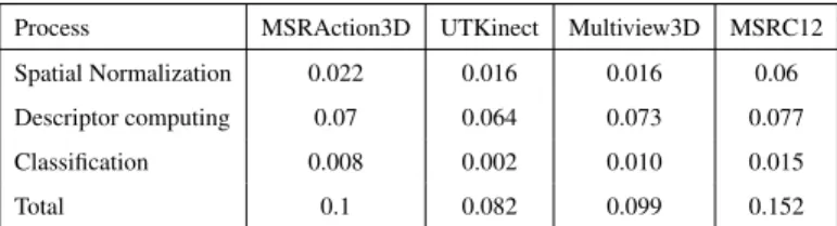
Process MSRAction3D UTKinect Multiview3D MSRC12 Spatial Normalization 0.022 0.016 0.016 0.06
Descriptor computing 0.07 0.064 0.073 0.077 Classification 0.008 0.002 0.010 0.015
Total 0.1 0.082 0.099 0.152
Table 2: Execution time (s) of each process per KSC-NPMSE-l1descriptor on the four benchmarks
Descriptor Accuracy (%) MET (s) HOG2 [6] 74.15 5.03 HON4D [7] 90.92 25.39 SNV [9] 79.80 1365.33 JP [8] 100 0.43 RJP [8] 97.98 1.91 Q [8] 88.89 1.40 LARP [8] 97.08 42.00 Random Forrest* [56] 87.90 -ST-LSTM* [21] 95 -KSC-NAE (ours) 84.00 0.08 KSC-NPMSE-l1(ours) 94.00 0.09 KSC-NPMSE-l2(ours) 96.00 0.10
Table 3: Accuracy of recognition and MET per descriptor on UTKinect dataset. *The values have been recovered from the state-of-the-art
Descriptor Accuracy (%) MET (s) Logistic Regression* [12] 91.2 -Covariance descriptor* [55] 91.7 -KSC-NAE (ours) 84.00 0.137 KSC-NPMSE-l1(ours) 93.22 0.134
KSC-NPMSE-l2(ours) 94.27 0.134
Table 4: Accuracy of recognition and MET per descriptor on MSRC12 dataset. *The values have been recovered from the state-of-the-art
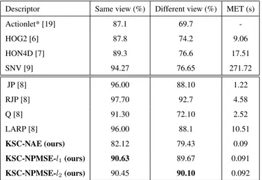
Descriptor Same view (%) Different view (%) MET (s) Actionlet* [19] 87.1 69.7 -HOG2 [6] 87.8 74.2 9.06 HON4D [7] 89.3 76.6 17.51 SNV [9] 94.27 76.65 271.72 JP [8] 96.00 88.10 1.22 RJP [8] 97.70 92.7 4.58 Q [8] 91.30 72.10 2.52 LARP [8] 96.00 88.1 10.51 KSC-NAE (ours) 82.12 79.43 0.09 KSC-NPMSE-l1(ours) 90.63 89.67 0.091 KSC-NPMSE-l2(ours) 90.45 90.10 0.092
Table 5: Accuracy of recognition and MET per descriptor on Multiview3D dataset. *The values have been recovered from the state-of-the-art
5.2. Results and discussion 5.2.1. Low computational latency
Table 1, Table 3, Table 4 and Table 5 compare our approach with state-of-the-art methods in terms of computational latency by reporting the MET per descriptor in respectively MSRAction3D, UTKinect, MSRC12 and Multiview3D datasets. As
men-420
tioned in [3], it has been shown that the skeleton extraction process lasts approximately 45ms/per frame with the knowledge that actions are generally contained in a window composed of 12 to 50 frames. Thus, a fair comparison of execution time would have consisted in adding a penalty of 2250 ms for skeleton methods. But, this would have no influence on the fact that our approach remains more suited to real-time
applica-425
tions, despite an additional extraction process. Indeed, we show that our descriptors KSC-NAE, KSC-NPMSE-l1and KSC-NPMSE-l2are faster in terms of computational latency with a maximum of only 0.092s of MET on MSRAction3D dataset, 0.10 on UTKinect dataset, 0.137 on MSRC12 dataset and 0.092 on Multiview3D dataset. Also, Table 2, which presents the execution time per descriptor of each process on the four
430
benchmarks. Since some state-of-the-art methods do not provide their codes, we added an asterisk in front of their name to indicate that the accuracy has been directly
re-covered from the associated papers (the experimental conditions can be different than ours). For this reason, we could not provide the MET required for these methods. However, in [35], the time of calculation required for each frame is reported. The
au-435
thors mention that the calculation of their descriptor takes about 2 seconds per frame (between 30 seconds and 100 seconds for a whole video of the MSRAction3D dataset). Knowing that the machine used for their experiments (3,4 GHz with 24 GB RAM) is largely more powerful than our laptop, one can say that the descriptors presented in our paper require less execution time.
440
Thus, with these results, we can assume that the constraint of low computational latency is respected. However, it is important to notice that the computational latency also depends from a lot of parameters such as the image resolution (from the number of joints, in this case) as well as the number of classes (20 for MSRAction3D, 10 for UTKinect, 12 for MSRC12 and 12 for Multiview3D datasets) and Table 1, Table 3,
Ta-445
ble 4 and Table 5 aim just at comparing execution time of different techniques applied to a similar situation.
5.2.2. Good accuracy and Robustness
Computational latency is an important criterion of evaluation, but is not sufficient. In fact, the accuracy of recognition must be acceptable. On the MSRAction3D, our
450
method allows us to recognize 89.64% of the actions correctly using KSC-NPMSE-l2descriptor, which is a better score than other skeleton representations. On the other hand, even if depth-based descriptors give better results in terms of accuracy of recogni-tion, their MET per descriptor remain too high and seem to be unsuitable for real-time applications (6.44s for HOG2, 27.333s for HON4D, 146.57s for SNV versus 0,092s
455
for KSC). Table 3, Table 9 and Table 4 respectively report the accuracy of recognition of our method on UTKinect, MSRC12 and Multiview3D datasets and compare it to state-of-the-art methods. While on UTKinect the accuracy of recognition using KSC-NPMSE-l2 descriptor is 96% (1% less than the highest score), the accuracy of our method on MSRC12 dataset outperforms recent state-of-the-art method with 94.27%
460
. On Multiview3D dataset, the accuracy of recognition given by the descriptor KSC-NPMSE-l2is also acceptable. When the training and testing are carried out using data
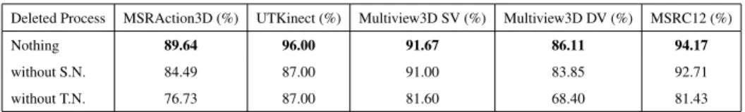
Deleted Process MSRAction3D (%) UTKinect (%) Multiview3D SV (%) Multiview3D DV (%) MSRC12 (%) Nothing 89.64 96.00 91.67 86.11 94.17 without S.N. 84.49 87.00 91.00 83.85 92.71 without T.N. 76.73 87.00 81.60 68.40 81.43
Table 6: Effect of each process on the accuracy of recognition using KSC-NPMSE-l2
with the Same Viewpoint (SV), the score of accuracy is equal to 91.67% (around 4% percent less than the highest score and 4% percent better than Actionlet). And when the training and testing use data with Different Viewpoints (DV), the recognition accuracy
465
is equal to 86.11% (versus 88.1% for LARP and 69.7% for Actionlet). As mentioned before, Table 2 shows that computational latency remains relatively low on the four datasets using our method. Thus, we can conclude that the performance of our descrip-tor is acceptable on the four benchmarks and that our method is robust to the dataset changing.
470
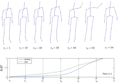
5.2.3. NAE vs NPMSE
Thanks to the experiments, we can conclude that the NMPSE function gives better results than the NAE function on the four datasets. Indeed, we can notice a difference of around 5% on MSRAction3D dataset, 12% of UTKinect dataset, 10% on MSRC12 dataset and 4% on Multiview3D dataset between the descriptors NAE and
KSC-475
NPMSE-l2, while the execution time per descriptor remains the same. Also, compared to the distance l1, the distance l2gives slightly more accurate results. In future work, it could be interesting to compare a wider range of more sophisticated distances. By observing the shape of the two curves (NAE and NPMSE-l2) as shown by Figure 6, it can be noticed that the NMPSE is smoother than NAE and that NMPSE increases
480
importantly only in the presence of key poses, while NAE increases more uniformly. The superiority of NMPSE as a TVRF function could be explained by the fact that the notion of key frames is more exploited with the use of NMPSE. In the rest of experiments, only the KSC-NPMSE-l2 will be taken into account since it gives the best results.
Figure 6: The visualization of the NAE (green) and the NPMSE (blue) varying over time. Skeletons at some instants tkare also visualized.
5.2.4. Benefits of Spatial Normalization (SN)
Table 9 reports the effect of the different processes of normalization. Each column of the table presents the obtained accuracy of recognition, after deleting one of the pro-posed processes contributing to spatial and temporal normalizations. We can observe that SN contributes considerably to increasing the accuracy on the three datasets. We
490
observe an increase of around 5% for MSRAction3D, 9% for UTKinect and approxi-mately 0.67% and around 2 % for Multiview3D (for respectively SV and DV tests) and more than 1% for MSRC12, when SN is used. To explain the use of unitary Euclidean normalization instead of the use of an average skeleton as in [43], we report the results of our method combined with an average skeleton-based normalization on the four
495
datasets used. The accuracy of recognition is very low compared with the values ob-tained using our spatial normalization algorithm with only 81.92% on MSRAction3D, 84% on UTKinect and 87.5%(SV) - 79.95% (DV) on Multiview3D.
Kinematics MSRAction3D (%) UTKinect (%) Multiview3D SV (%) Multiview3D DV (%) MSRC12 (%) P+V+A 89.64 96.00 91.67 86.11 94.17 P+V 86.06 92.00 90.63 82.64 93.92 P 86.04 90.00 86.98 70.05 93.50 V 83.01 90.00 85.07 78.56 89.68 A 82.39 81.00 83.33 77.78 86.46
Table 7: Effect of each kinematic component on the accuracy of recognition using KSC-NPMSE-l2
5.2.5. Benefits of Temporal Normalization (TN): the TVR algorithm
In Table 5, the removal of the TN process (TVR algorithm) shows its important role
500
in our method. Indeed, without TN, the accuracy of recognition decreases from 89.64% to 76.73% on MSRAction 3D, from 96% to 87% on UTKinect, from 91.67%(SV)-86.11%(DV) to 81.60%(SV)-68.40%(DV) on Multiview3D and from 94.17% to 81.43%. These results confirm the ability of our algorithm to cope with execution rate variabil-ity. This algorithm is very useful for pre-segmented actions, since it is fast and efficient.
505
However, to work efficiently, the video should start with a skeleton in a rest state. In-deed, the calculation of the NPMSE term, which quantifies the important phase of the motion, is based on this assumption.
5.2.6. Benefits of kinematic features
In Table 7, we evaluate the importance of each kinematic term. This table shows
510
that position is generally the most discriminative value followed by velocity and ac-celeration. This may be due to the increase of the approximation error caused by the derivations. Nevertheless, the combined information of the three kinematic values give us the best amount of accuracy on the four datasets.
5.2.7. Parameters influence
515
The parameter s, which represents the number of samples affects the accuracy of recognition. As shown in the Table 8, with varying the parameter s, the accuracy of recognition will also vary. The parameter s is therefore fixed according to the best score obtained ( s = 15 for MSRAction3D, UTKinect and Multiview3D and s = 40 for MSRC12). If s is fixed too small, the accuracy decreases because of a loss of
numberof sampless 5 (%) 10 (%) 15 (%) 20 (%) 25 (%) 30 (%) 35 (%) 40 (%) 45 (%) 50 (%) MSRAction3D 86.03 86.90 89.64 88.75 88.46 88.14 87.55 87.86 86.96 86.94 UTKinect 94.00 95.00 96.00 93.00 95.00 95.00 95.00 94.00 94.00 94.00 Multiview3D (SV) 88.54 90.28 91.67 90.45 89.58 89.76 89.76 90.10 90.10 90.10 Multiview3D (DV) 83.51 85.07 86.11 84.11 84.20 84.72 84.38 84.55 84.37 84.46 MSC12 92.20 92.96 93.91 93.92 93.69 94.04 94.11 94.17 94.08 93.98
Table 8: Effect of s the number of samples s on the accuracy of recognition using KSC-NPMSE-l2
information. On the other hand, if s is too high, the accuracy also decreases since the influence of the interpolation errors increases. Indeed, the original data is numerical and has been interpolated. Nevertheless, is important to notice that the choice of s does not affect the results considerably. For the values tested, we observe a decrease of up to 3% compared with the highest score of accuracy for a number of samples varying
525
between 5 and 50.
5.3. Performance on a large-scale dataset: NTU + RGB-D dataset
In this part, we propose to test our method on the recent large-scale action recogni-tion benchmark: NTU-RGB+D dataset. Because of the important amount of data, we use for this experimentation another laptop: an i7 macbook pro with 16 Go of RAM.
530
Since this dataset contains mutual actions involving more than one human, only the skeleton consuming more kinetic energy is considered. On the other hand, some joints are sometimes confused and have exactly the same coordinates. To overcome that, a small Gaussian noise is added to one of the two joints. We follow the same experimen-tal protocol used in [16] and we propose to report the accuracy in Table 9 obtained for
535
the two settings: cross-subject and cross-view. Compared to hand-crafted methods, our approach reaches the best score of accuracy while realizing the cross-subject test (with 51.12 %) and the second best score while performing cross-view test (with 51.39 %, slightly inferior to the accuracy obtained for the Lie Group [8] representation 52.76 %). We specify that the parameter s has been fixed to 20. Despite the promising results, it
540
can be noted in Table 9 that methods based on learned features remain more efficient on this dataset in terms of accuracy.
Class of method Method Cross-subject (%) Cross-view (%) hand-crafted HOG2 [6] 32.24 22.27 SNV [9] 31.82 13.61 HON4D [7] 30.56 7.26 Lie Group [8] 50.08 52.76 Skeletal Quads [57] 38.62 41.36 KSC-NMPSE-l2(ours) 51.12 51.39 learned features HBRNN-L [58] 59.07 63.97 ST-LSTM [21] 69.2 77.7 SkeletonNet [22] 75.94 81.16 Rahmani et al. [59] 75.2 83.1 Clips + CNN + MTLN [20] 79.57 84.83
Table 9: Accuracy of recognition of different methods on NTU-RGB+D
6. Conclusion and future work
In this work, we have presented a novel descriptor for fast action recognition. It is based on the cubic spline interpolation of kinematic values of joints, more precisely,
545
position, velocity and acceleration. To make our descriptor invariant to anthropometric variability and execution rate variation, we perform a skeleton normalization as well as a temporal normalization. For this reason, a novel method of temporal normalization is proposed called TVR. The proposed method have shown its efficiency in terms of accuracy and computational latency on four different datasets.
550
However, actions are assumed to be already segmented. In future work, the issue of temporal segmentation will be studied. Some techniques developed for dynamical switched models can be used to detect different modes in an unsegmented sequence, allowing the detection of particular points of transition from an action to another or from an action to the rest state. First attempts have been made to adapt these methods
555
in [60, 61, 62, 23].
References
[1] R. Poppe, A survey on vision-based human action recognition, Image and Vision Computing 28 (6) (2010) 976–990.
[2] D. Weinland, R. Ronfard, E. Boyer, A survey of vision-based methods for
ac-560
tion representation, segmentation and recognition, Computer Vision and Image Understanding 115 (2) (2011) 224–241.
[3] G. T. Papadopoulos, A. Axenopoulos, P. Daras, Real-time skeleton-tracking-based human action recognition using kinect data, in: International Conference on Multimedia Modeling, Springer, 2014, pp. 473–483.
565
[4] E. Ghorbel, R. Boutteau, J. Boonaert, X. Savatier, S. Lecoeuche, 3D real-time human action recognition using a spline interpolation approach, in: International Conference on Image Processing Theory Tools and Applications, IEEE, 2015. [5] W. Li, Z. Zhang, Z. Liu, Action recognition based on a bag of 3D points, in:
Con-ference on Computer Vision and Pattern Recognition Workshops, IEEE, 2010,
570
pp. 9–14.
[6] E. Ohn-Bar, M. M. Trivedi, Joint angles similarities and HOG2 for action recog-nition, in: Conference on Computer Vision and Pattern Recognition Workshops, IEEE, 2013, pp. 465–470.
[7] O. Oreifej, Z. Liu, HON4D: Histogram of oriented 4D normals for activity
recog-575
nition from depth sequences, in: Conference on Computer Vision and Pattern Recognition, IEEE, 2013, pp. 716–723.
[8] R. Vemulapalli, F. Arrate, R. Chellappa, Human action recognition by represent-ing 3D skeletons as points in a Lie group, in: Conference on Computer Vision and Pattern Recognition, IEEE, 2014, pp. 588–595.
580
[9] X. Yang, Y. Tian, Super Normal Vector for activity recognition using depth se-quences, in: Conference on Computer Vision and Pattern Recognition, IEEE, 2014, pp. 804–811.
[10] S. J. Kim, S. W. Kim, T. Sandhan, J. Y. Choi, View invariant action recognition using generalized 4D features, Pattern Recognition Letters 49 (2014) 40–47.
[11] J. Luo, W. Wang, H. Qi, Spatio-temporal feature extraction and representation for RGB-D human action recognition, Pattern Recognition Letters 50 (2014) 139– 148.
[12] C. Ellis, S. Z. Masood, M. F. Tappen, J. J. Laviola Jr, R. Sukthankar, Exploring the trade-off between accuracy and observational latency in action recognition,
590
International Journal of Computer Vision, Springer 101 (3) (2013) 420–436. [13] L. Xia, C.-C. Chen, J. Aggarwal, View invariant human action recognition using
histograms of 3D joints, in: Conference on Computer Vision and Pattern Recog-nition Workshops, IEEE, 2012, pp. 20–27.
[14] S. Fothergill, H. Mentis, P. Kohli, S. Nowozin, Instructing people for training
595
gestural interactive systems, in: SIGCHI Conference on Human Factors in Com-puting Systems, ACM, 2012, pp. 1737–1746.
[15] M. Hammouche, E. Ghorbel, A. Fleury, S. Ambellouis, Toward a real time view-invariant 3d action recognition, in: International Joint Conference on Computer Vision, Imaging and Computer Graphics Theory and Applications, 2016.
600
[16] A. Shahroudy, J. Liu, T.-T. Ng, G. Wang, NTU RGB+D: A large scale dataset for 3D human activity analysis, in: Conference on Computer Vision and Pattern Recognition, IEEE, 2016, pp. 1010–1019.
[17] E. Ghorbel, R. Boutteau, J. Bonnaert, X. Savatier, S. Lecoeuche, A fast and accu-rate motion descriptor for human action recognition applications, in: International
605
Conference on Pattern Recognition, IEEE, 2016, pp. 919–924.
[18] F. Zhu, L. Shao, J. Xie, Y. Fang, From handcrafted to learned representations for human action recognition: a survey, Image and Vision Computing 55 (2016) 42–52.
[19] J. Wang, Z. Liu, Y. Wu, J. Yuan, Mining actionlet ensemble for action recognition
610
with depth cameras, in: Conference on Computer Vision and Pattern Recognition, IEEE, 2012, pp. 1290–1297.
[20] Q. Ke, M. Bennamoun, S. An, F. Sohel, F. Boussaid, A new representation of skeleton sequences for 3D action recognition, in: Conference on Computer Vision and Pattern Recognition, IEEE, 2017, pp. 4570–4579.
615
[21] J. Liu, A. Shahroudy, D. Xu, G. Wang, Spatio-temporal LSTM with trust gates for 3D human action recognition, in: European Conference on Computer Vision, Springer, 2016, pp. 816–833.
[22] Q. Ke, S. An, M. Bennamoun, F. Sohel, F. Boussaid, Skeletonnet: Mining deep part features for 3-D action recognition, Signal Processing Letters, IEEE 24 (6)
620
(2017) 731–735.
[23] Z. Liu, C. Zhang, Y. Tian, 3D-based deep convolutional neural network for action recognition with depth sequences, Image and Vision Computing 55 (2016) 93– 100.
[24] R. Qiao, L. Liu, C. Shen, A. Van Den Hengel, Learning discriminative
trajecto-625
rylet detector sets for accurate skeleton-based action recognition, Pattern Recog-nition 66 (2017) 202–212.
[25] L. Xia, J. Aggarwal, Spatio-temporal depth cuboid similarity feature for activity recognition using depth camera, in: Conference on Computer Vision and Pattern Recognition, IEEE, 2013, pp. 2834–2841.
630
[26] S. Belongie, K. Branson, P. Dollar, V. Rabaud, Monitoring animal behavior in the smart vivarium, in: Measuring Behavior, 2005, pp. 70–72.
[27] P. Doll´ar, V. Rabaud, G. Cottrell, S. Belongie, Behavior recognition via sparse spatio-temporal features, in: International Workshop on Visual Surveillance and Performance Evaluation of Tracking and Surveillance, IEEE, 2005, pp. 65–72.
635
[28] N. Dalal, B. Triggs, Histograms of oriented gradients for human detection, in: Conference on Computer Vision and Pattern Recognition, IEEE, Vol. 1, 2005, pp. 886–893.
[29] A. Klaser, M. Marszałek, C. Schmid, A spatio-temporal descriptor based on 3D-gradients, in: British Machine Vision Conference, 2008, pp. 275–1.
640
[30] A. M. Sabri, J. Boonaert, S. Lecoeuche, E. Mouaddib, Human action classifi-cation using surf based spatio-temporal correlated descriptors, in: International Conference on Image Processing, IEEE, 2012, pp. 1401–1404.
[31] V. Bettadapura, G. Schindler, T. Pl¨otz, I. Essa, Augmenting bag-of-words: Data-driven discovery of temporal and structural information for activity recognition,
645
in: Conference on Computer Vision and Pattern Recognition, IEEE, 2013, pp. 2619–2626.
[32] P. Foggia, G. Percannella, A. Saggese, M. Vento, Recognizing human actions by a bag of visual words, in: International Conference on Systems, Man, and Cybernetics, IEEE, 2013, pp. 2910–2915.
650
[33] P. Shukla, K. K. Biswas, P. K. Kalra, Action recognition using temporal bag-of-words from depth maps, in: International Conference on Machine Vision Appli-cations, IEEE, 2013, pp. 41–44.
[34] L. Brun, G. Percannella, A. Saggese, M. Vento, Action recognition by using ker-nels on aclets sequences, Computer Vision and Image Understanding 144 (2016)
655
3–13.
[35] H. Rahmani, A. Mahmood, D. Huynh, A. Mian, Histogram of oriented principal components for cross-view action recognition, Transactions on Pattern Analysis and Machine Intelligence, IEEE 38 (12) (2016) 2430–2443.
[36] R. Slama, H. Wannous, M. Daoudi, Grassmannian representation of motion depth
660
for 3D human gesture and action recognition, in: International Conference on Pattern Recognition, IEEE, 2014, pp. 3499–3504.
[37] H. S. M. Coxeter, Regular polytopes, Courier Corporation, 1973.
[38] X. Yang, Y. Tian, Eigenjoints-based action recognition using Naive-bayes-Nearest-Neighbor, in: Conference on Computer Vision and Pattern Recognition
665
[39] M. Devanne, H. Wannous, S. Berretti, P. Pala, M. Daoudi, A. Del Bimbo, 3-D human action recognition by shape analysis of motion trajectories on Riemannian manifold, Transactions on Cybernetics, IEEE 45 (7) (2015) 1340–1352.
[40] M. Devanne, S. Berretti, P. Pala, H. Wannous, M. Daoudi, A. Del Bimbo, Motion
670
segment decomposition of RGB-D sequences for human behavior understanding, Pattern Recognition 61 (2017) 222–233.
[41] G. Johansson, Visual perception of biological motion and a model for its analysis, Perception & psychophysics, Springer 14 (2) (1973) 201–211.
[42] R. Vemulapalli, F. Arrate, R. Chellappa, R3DG features: Relative 3D
geometry-675
based skeletal representations for human action recognition, Computer Vision and Image Understanding 152 (2016) 155–166.
[43] M. Zanfir, M. Leordeanu, C. Sminchisescu, The moving pose: An efficient 3D kinematics descriptor for low-latency action recognition and detection, in: Inter-national Conference on Computer Vision, IEEE, 2013, pp. 2752–2759.
680
[44] C. De Boor, Spline toolbox for use with MATLAB: user’s guide, version 3, Math-Works, 2005.
[45] K. Onuma, C. Faloutsos, J. K. Hodgins, FMDistance: A fast and effective dis-tance function for motion capture data., in: Eurographics, 2008, pp. 83–86. [46] J. Shan, S. Akella, 3D human action segmentation and recognition using pose
685
kinetic energy, in: Workshop on Advanced Robotics and its Social Impacts, IEEE, 2014, pp. 69–75.
[47] Y. Shi, Y. Wang, A local feature descriptor based on energy information for hu-man activity recognition, in: Advanced Intelligent Computing Theories and Ap-plications, Springer, 2015, pp. 311–317.
690
[48] L. Miranda, T. Vieira, D. Martinez, T. Lewiner, A. W. Vieira, M. F. Campos, Real-time gesture recognition from depth data through key poses learning and
decision forests, in: SIBGRAPI Conference on Graphics, Patterns and Images, IEEE, 2012, pp. 268–275.
[49] N. P. Cuntoor, R. Chellappa, Key frame-based activity representation using
695
antieigenvalues, in: Asian Conference on Computer Vision, Springer, 2006, pp. 499–508.
[50] M. Raptis, D. Kirovski, H. Hoppe, Real-time classification of dance gestures from skeleton animation, in: SIGGRAPH/Eurographics symposium on computer ani-mation, ACM, 2011, pp. 147–156.
700
[51] C.-C. Chang, C.-J. Lin, LIBSVM: A library for Support Vector Machines, Trans-actions on Intelligent Systems and Technology, ACM 2 (3) (2011) 27.
[52] K. Crammer, Y. Singer, On the learnability and design of output codes for multi-class problems, Machine learning, Springer 47 (2-3) (2002) 201–233.
[53] S. R. Fanello, I. Gori, G. Metta, F. Odone, Keep it simple and sparse:
Real-705
time action recognition, The Journal of Machine Learning Research 14 (1) (2013) 2617–2640.
[54] J. R. Padilla-L´opez, A. A. Chaaraoui, F. Fl´orez-Revuelta, A discussion on the validation tests employed to compare human action recognition methods using the MSR Action3D dataset, arXiv preprint arXiv:1407.7390.
710
[55] M. E. Hussein, M. Torki, M. A. Gowayyed, M. El-Saban, Human action recog-nition using a temporal hierarchy of covariance descriptors on 3D joint locations, in: International Joint Conferences on Artificial Intelligence, Vol. 13, 2013, pp. 2466–2472.
[56] Y. Zhu, W. Chen, G. Guo, Fusing spatiotemporal features and joints for 3D
ac-715
tion recognition, in: Conference on Computer Vision and Pattern Recognition Workshops, IEEE, 2013, pp. 486–491.
[57] G. Evangelidis, G. Singh, R. Horaud, Skeletal quads: Human action recogni-tion using joint quadruples, in: Internarecogni-tional Conference on Pattern Recognirecogni-tion, IEEE, 2014, pp. 4513–4518.
[58] Y. Du, W. Wang, L. Wang, Hierarchical recurrent neural network for skeleton based action recognition, in: Conference on Computer Vision and Pattern Recog-nition, IEEE, 2015, pp. 1110–1118.
[59] H. Rahmani, M. Bennamoun, Learning action recognition model from depth and skeleton videos, in: Conference on Computer Vision and Pattern Recognition,
725
IEEE, 2017, pp. 5832–5841.
[60] K. Boukharouba, L. Bako, S. Lecoeuche, Temporal video segmentation using a switched affine models identification technique, in: International Conference on Image Processing Theory Tools and Applications, IEEE, 2010, pp. 157–160. [61] F. Ofli, R. Chaudhry, G. Kurillo, R. Vidal, R. Bajcsy, Sequence of the most
infor-730
mative joints (SMIJ): A new representation for human skeletal action recognition, Journal of Visual Communication and Image Representation 25 (1) (2014) 24–38. [62] R. Vidal, S. Soatto, A. Chiuso, Applications of hybrid system identification in computer vision, in: European Control Conference, IEEE, 2007, pp. 4853–4860.

![Table 1: Accuracy of recognition and execution time per descriptor(s) on MSRAction3D: AS1, AS2 and AS3 represents the three groups proposed in the protocol experimentation of [5]](https://thumb-eu.123doks.com/thumbv2/123doknet/12434093.334785/23.918.265.658.185.434/accuracy-recognition-execution-descriptor-msraction-represents-proposed-experimentation.webp)