HAL Id: hal-01982609
https://hal.laas.fr/hal-01982609
Submitted on 15 Jan 2019
HAL is a multi-disciplinary open access
archive for the deposit and dissemination of sci-entific research documents, whether they are pub-lished or not. The documents may come from
L’archive ouverte pluridisciplinaire HAL, est destinée au dépôt et à la diffusion de documents scientifiques de niveau recherche, publiés ou non, émanant des établissements d’enseignement et de
Enhancing systematic protein-protein docking methods
using ray casting: Application to ATTRACT
Yi Li, Juan Cortés, Thierry Simeon
To cite this version:
Yi Li, Juan Cortés, Thierry Simeon. Enhancing systematic protein-protein docking methods using ray casting: Application to ATTRACT. Proteins - Structure, Function and Bioinformatics, Wiley, 2011, 79 (11), pp.3037-3049. �10.1002/prot.23127�. �hal-01982609�
Enhancing Systematic Protein-Protein
Docking Methods using Ray Casting:
Application to ATTRACT
Yi Li, Juan Cort´es, and Thierry Sim´eon
1CNRS; LAAS; 7 avenue du colonel Roche, F-31077 Toulouse, France
Universit´e de Toulouse; UPS, INSA, INP, ISAE; LAAS;
F-31077 Toulouse, France
July 15, 2011
1Correspondence to: Thierry Sim´eon; CNRS; LAAS; 7 avenue du colonel Roche,
F-31077 Toulouse, France; E-mail: [email protected]; Phone: +33 5 61 33 63 49; Fax : +33 5 61 33 64 55.
Abstract
Systematic protein-protein docking methods need to evaluate a huge number of different probe configurations, thus leading to high computational cost. We present an efficient filter — Ray Casting Filter (RCF) — that enables a notable speed-up of systematic protein-protein docking. The high efficiency of RCF is the outcome of the following factors: (i) extracting of pockets and protrusions on the surfaces of the proteins using visibilities; (ii) a ray casting method that finds aligned recep-tor pocket/probe protrusion pairs without explicit similarity computations. The RCF method enables the integration of systematic methods and local shape fea-ture matching methods. To verify the efficiency and the accuracy of RCF, we in-tegrated it with a systematic protein-protein docking approach (ATTRACT) based on a reduced protein representation. The test results show that the integrated docking approach is much faster. At the same time, it ranks the lowest ligand RMSD (L rms) solutions higher when docking enzyme-enzyme inhibitor com-plexes. Consequently, RCF not only enables much faster execution of systematic docking runs but also improves the qualities of docking predictions.
Keywords: protein-protein interaction; protein docking; protein interaction
geometry; biomolecular simulation; ray casting.
Introduction
Proteins are essential biological macromolecules that participate in most of the processes within cells. A better understanding of how proteins interact with each
other (i.e., protein-protein docking) at the atomic level will lead to major scientific advances, with important applications in medicine, pharmacology, and biotech-nology. However, available tools that provide structural information on how pro-teins interact with other molecules are still very limited. Experimental methods such as X-ray crystallography and nuclear magnetic resonance (NMR) are able to obtain an atomic-resolution representation of proteins, but provide very limited information about how proteins interact. Furthermore, it is often more difficult to determine protein complexes experimentally than their isolated components. Thus, the number of experimentally solved protein complexes is still small, which has motivated the development of in silico approaches to investigate the protein-protein docking problem. However, this research remains at the theoretical stage for the time being, because predictions given by the docking methods proposed so far still contain false positives and negatives [1].
The general scheme of flexible docking consists of four major stages [2]. In the first stage, the proteins’ conformational space (i.e., the degrees of freedom to be searched such as global translations and rotations, side-chain rotations, etc.) is defined. The second stage consists of performing a conformational search with the aim of finding candidate structures of the complex. Usually, the two proteins are treated as rigid bodies in this stage. One protein (usually the smaller one) — the ligand protein — is often used as the probe, while the other protein is the receptor and remains fixed during the docking process. In the third stage, each candidate is refined by taking into account backbone flexibility and side-chain flexibility [3, 4, 5] in addition to rigid-body adjustments. Finally, the fourth
and last stage aims to identify the near-native solutions among the candidates by re-scoring and re-ranking them using a more expensive and more accurate scoring function. For a detailed description of available methods, we refer to some excellent review articles [1, 6, 7, 8, 9, 2].
In this paper, we focus on rigid-docking, because refinement using flexible models are futile if the rigid-docking stage does not produce any near-native struc-ture among the top-ranked solution candidates. When docking two proteins as rigid bodies, a set of candidate structures is identified by either matching local shape features [10, 11, 12, 13, 14, 15, 16, 17, 18] or enumerating the transforma-tion space systematically (i.e., by brute force) [19, 20, 21, 22, 3].
The local shape feature matching method presented in [12] uses a soft-potential-based steric scoring scheme to assess surface complementarity between antibody-antigen complexes. Methods that match local curvature maxima and minima points have been studied in [11, 13, 14]. Robust definitions of the curvature can also be provided by a Voronoi-diagram-based model [18] of macromolecu-lar interfaces in addition to the connectivity of the interfaces. Methods that can model proteins with flexibility have been presented in [15, 16]. Even though a more recent method called PatchDock [17] is able to dock some unbound pro-teins by matching geometric patches (concave, convex, and flat surface pieces), local-shape-feature-matching-based methods are usually not sufficient when the structures are unbound [7].
When docking two proteins systematically, a huge number of possible probe geometries, in terms of relative orientation and position to the receptor, must be
evaluated. The problem increases in complexity when internal degrees of freedom (DOFs) also need to be explored, in which case the use of some previously devel-oped search algorithms leads to computational explosion. For example, methods based on the fast Fourier transform (FFT) [19, 20, 21, 22, 23] can take many CPU-hours to execute, because even though the FFT is used to rapidly enumer-ate the translations of the probe, rotations are still being searched systematically. ATTRACT [3], another systematic method, is based on a reduced protein repre-sentation and it docks a probe and a receptor by energy minimization. For each systematic docking run, it generates a large number of start configurations by placing the probe at various positions on the surface of the receptor and then gen-erating many probe orientations for each position. For each start configuration, energy between the probe and the receptor is minimized in the probe’s rotational and translational degrees of freedom. It can also take several CPU-hours for AT-TRACT to dock two proteins, but it has no problem with residual unfavorable interactions caused by the discrete sampling of rotational degrees of freedom (as done by the FFT based methods).
In this paper, we propose an efficient filter that utilizes ray casting — which we have named Ray Casting Filter (RCF) — to enhance systematic docking meth-ods. The RCF method enables the integration of systematic methods and local shape feature matching methods. First, the protein surface areas (such as pockets and protrusions) that are likely part of the binding site are identified by checking local shape features. Then for each configuration of the probe, RCF is applied to verify whether complementary surface areas on the probe and on the
recep-tor are aligned (e.g., whether a surface area on the probe of type protrusion is aligned with a surface area on the receptor of type pocket). If no correct align-ment is found, the configuration can be safely discarded, thus eliminating the need to carry out further operations (e.g., energy minimizations) from this configura-tion. We have to point out that a binding pocket does not necessarily have roughly the same area as the corresponding binding protrusion, at least not for the areas of pockets and protrusions identified by our method. Consequently, protrusion-pocket area similarity is not used in RCF as a criterion. To verify the efficiency and the accuracy of RCF, we implemented RCF-ATTRACT by integrating the filter with ATTRACT [3] and tested it on both the bound-bound cases and the unbound-unbound cases of [3], which mainly consist of enzyme-enzyme inhibitor complexes. Furthermore, since many drug molecules are enzyme inhibitors and hence docking of enzyme-enzyme inhibitor complexes is very important in drug design, the implementation presented in this paper focuses on this type of protein complexes by looking for receptor pocket/probe protrusion pairs using RCF. Our results show that the integrated method is much faster, and that its lowest L rms solutions for enzyme-enzyme inhibitor complexes are similar to the ones obtained by ATTRACT. Moreover, these solutions are ranked higher by RCF-ATTRACT.
Materials and Methods
When docking two proteins, the systematic docking methods initialize a huge number of configurations for the probe, and then for each configuration, the
com-plementarity between the proteins is checked. In this section, we propose a filter-ing approach to avoid expensive operations such as complementarity checks (e.g., the calculation of the correlation function performed by the FFT-based methods) and energy minimizations done by the systematic docking methods. Essentially, we look for aligned receptor pocket/probe protrusion pairs by casting virtual light rays (inspired by ray casting [24] from the field of computer graphics) toward both the probe and the receptor. This operation is extremely fast because no explicit similarity computation between protrusions and pockets is required by RCF. The probe configurations that do not give rise to any aligned pair are rejected, and hence many expensive operations are avoided.
RCF has two major stages: (i) characterization of local geometry of protein surfaces (i.e., compute surface meshes of the proteins and then divide them into three distinct areas: pockets, protrusions, and flat regions) and (ii) finding aligned receptor pocket/probe protrusion pairs with ray casting. At the end of the section, we show that the efficiency of the filter can be dramatically improved using a two-pass ray casting approach.
Characterizing local geometry of protein surfaces
Inspired by VisGrid [25], we use a visibility criterion to characterize local ge-ometry of protein surfaces. However, instead of voxelizing a protein structure as done by VisGrid, we compute protein surface mesh using MSMS [26, 27]. The advantage of using a surface mesh is that it permits a more efficient intersection detection with rays in both stages of the method.
Once the triangulated surface mesh has been computed by MSMS, the visi-bility of each mesh vertex is determined by shooting rays and then counting the number of rays that intersect with the mesh. As shown in Fig. 1, for each vertex P of the surface mesh, P is slightly shifted in the direction of the surface normal N at the vertex to obtain point Q = P + ¡N, where ¡ is a small positive number. Next,
n uniformly distributed rays are shot from Q (following the method presented
in [28]) and intersections with the surface mesh are checked using an efficient collision detection algorithm called PQP [29, 30]. In order to divide the surface meshes into pockets, protrusions, and flat regions, we define two thresholds: pmin and pmax such that 0 < pmin< pmax < 1. If the percentage p of rays that intersect with the mesh is less than pmin, the visibility (1− p) at the vertex is considered to be good. On the other hand, if p > pmax, the visibility at the vertex is considered to be poor. r3 r2 r1 rn r5 r7 r6 r4 ! Q P N
Figure 1: The visibility at the vertex P is determined by shooting uniformly dis-tributed rays from Q and then checking for intersections with the surface mesh.
visibil-ity of its three vertices. If two or three vertices of a mesh triangle have good/poor visibility, the type of the triangle is set to protrusion/pocket. Two adjacent trian-gles of the same type that share a common edge are then merged into one group. Thus, a pocket corresponds to a set of grouped triangles with poor visibility. Sim-ilarly, a protrusion corresponds to a set of grouped triangles with good visibility. The rest of the surface is identified as flat regions. Note that even though it is possible that a large patch of triangles of a certain signature may enclose a few mismatched triangles, the experimental results show that RCF does not rely on topologies of surface patches to work properly. Furthermore, a minimum area threshold could be defined to avoid very small protrusions/pockets.
Since the identified protrusions and pockets are used later to verify whether the probe at one particular configuration is aligned with the receptor (i.e., likely to dock), pminand pmax have to be chosen carefully. Extensive tests have shown that
pmin= 0.40 and pmax= 0.75 are suitable for the identification of probe protrusions and receptor pockets, respectively. For example, the identified 2PTC receptor pockets and 2PTC probe protrusions are displayed in Fig. 2. With larger values for pmax (e.g., pmax = 0.85), only the deepest part of the docking pocket on the 2PTC receptor is classified as pocket, which means that the probability that virtual rays miss the docking pocket is greater. Similarly, with lower values for pmax (e.g., pmax= 0.65), many relatively shallow parts of the receptor surface are also classified as pockets, which degrades the efficiency of RCF and leads to longer docking time. When pmin = 0.30, only tips of many protrusions on the 2PTC probe are classified as protrusions. Consequently, they may be difficult to be
detected by rays. Conversely, more surface areas than necessary are classified as protrusions when pmin= 0.50. The influence of the parameter setting is discussed in depth at the end of the Results and Discussion section.
Next, the largest pockets that are likely to be involved in the docking are iden-tified. The pockets are divided into two sets. Slarge contains pockets with large areas, while Ssmall contains all pockets that are not part of Slarge. The threshold that divides the pockets into the two sets is set to 0.40Amax, where Amaxis the area of the largest pocket. A receptor pocket belongs to Slargeif its area is larger than this threshold. For enzyme-enzyme inhibitor complexes, which are the focus of this paper, the hypothesis is that the area of the docking enzyme pocket should only be slightly smaller than the largest one, if it is not the largest one itself. As shown in supplementary material, there are very few large pockets on enzyme sur-faces, and most of the pockets are very small compared to the ones in Slarge. Note that our approach is different to the one used by VisGrid, which only considers the three largest pockets. Our approach is more conservative in the sense that it often assigns more than three pockets to Slargewhen the largest pockets have very similar areas.
Finally, we point out that precise mathematical studies of protrusions and pockets have been performed in [31, 32, 33]. In [31], the definitions of protru-sions and pockets, according to Connolly, were recast in the framework of Morse theory. It also bridged the gap between Connolly’s definition and the curvature of molecular surfaces. Protrusions and pockets were defined from a canonical height function (i.e., a height function which does not depend on a predefined
z-(a) pmax= 0.65. (b) pmin= 0.30.
(c) pmax= 0.75. (d) pmin= 0.40.
(e) pmax= 0.85. (f) pmin= 0.50.
Figure 2: The three figures on the left show impact of pmaxon the classification of the 2PTC receptor pockets, where the pockets are shown as the red (dark gray in black/white print) regions. The three figures on the right show impact of pmin on the classification of the 2PTC probe protrusions, where the protrusions are shown as the blue (dark gray in black/white print) region.
axis) in [32]. A conception of surface curvature was defined in [33] by the alpha shape framework and then applied to the characterization of the molecular surface topography. However, our approach is much easier to implement, and it incorpo-rates non-local information (i.e., the visibility information) as opposed to strictly local information used by the aforementioned methods.
Finding aligned pocket/protrusion pairs
Our ray-casting-based method that finds all aligned large receptor pocket/probe protrusion pairs consists of two stages. First, rays are cast from the probe at a given position toward the receptor. We emphasize that this initial stage of ray casting is not done for each configuration of the probe, but only for each position, because a position in many systematic docking methods such as ATTRACT [3] is shared by multiple configurations (having different orientations). If a large pocket is detected by the rays on the receptor surface, a second stage of ray casting is executed, but this time the directions of the rays are reversed and they travel toward the probe. Ray casting in this second stage is repeated for each possible orientation of the probe, while its position remains unchanged, in order to detect probe orientations that align protrusions on the probe with the detected pocket(s) on the receptor. Note that the probe orientations at a given position are evaluated if and only if the evaluation of the position in the first stage has resulted in at least one receptor pocket. For example, in Fig. 3.a, the rays hit a flat region on the receptor and hence no rays are cast in the opposite direction toward the probe and all orientations of the probe can be discarded. In Fig. 3.b, a pocket on the
receptor has been detected, although no probe protrusion is aligned with it for that particular probe orientation. The pocket and the protrusion in Fig. 3.c are aligned, and hence the probe configuration has to be kept. The two stages are detailed next.
Receptor Probe Protrusion Rays Pocket Pr Pp
(a) Rays cast to-ward the receptor detect no pocket. Pocket Protrusion Rays Probe Receptor Pr Pp
(b) Rays cast toward the probe detect no protrusion.
Pocket Rays Receptor Protrusion Probe Pr Pp
(c) Rays cast toward the probe detect one protru-sion.
Figure 3: When no aligned receptor pocket/probe protrusion pairs are found for a probe configuration (e.g., the cases of the sub-figures a and b), the configuration can be safely discarded. Note that the probe orientations are explored only in the cases of the sub-figures b and c, not in the case of the sub-figure a.
The aim of the first stage is to identify potential large pockets on the receptor by placing the probe at a given position and then casting rays toward the receptor. Let the receptor position and the current position of the probe be denoted as Pr and Pp(the geometrical centers of the proteins), respectively. As shown in Fig. 4, a vector Vrayis defined by Prand Pp. Plane W is perpendicular to Vrayand passes through point Pp. m points are then sampled uniformly inside a disk on plane W. The disk is centered at Pp and it has a radius of rray= hrprobe, where rprobe is the radius of the probe’s bounding sphere and the values of the parameter h are discussed later. Next, m parallel rays are emitted from the sampled points
toward the receptor in the direction of Vray. Intersections between each ray and the surface mesh of the receptor are checked until the plane that is perpendicular to
Vray and passes through point Pr. Note that m is such that the maximum distance between two neighboring rays is 0.5 ˚A, which is short enough so that an atom is unlikely to be missed by the rays.
Receptor Probe Disk Pr Plane Π rray m rays Pp Vray
Figure 4: Parallel rays are cast from plane W toward the receptor protein in the direction of Vrayto detect large receptor pockets.
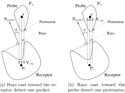
Rays cast towards the receptor are aimed at identifying interesting pockets. Note that a pocket is considered to be intersected by a ray as long as there is an intersection between them, and hence this intersection is not necessarily the first one between the receptor surface and the ray. If an intersection occurs between the pocket and the ray, the pocket is eliminated if e > emax, where e is the angle between−Vrayand the normal of the pocket Npocket (see Fig. 5.a), and emaxis the cutoff angle. The reason for this is that the probe is less likely to dock with the receptor at that particular pocket from the current probe position when e is large,
Protrusion Rays Receptor Probe θ Npocket Pr Pp Vray
(a) Rays cast toward the re-ceptor detect one pocket.
Protrusion Rays Receptor Probe Pp θ Npocket Pr −Vray
(b) Rays cast toward the probe detect one protrusion.
Figure 5: Ray casting is used to determine whether a pocket/protrusion pair (if any) is aligned. Note that the orientation of the probe is not important in the sub-figure a as only its position is used for ray casting in the first stage. However, in the second stage, ray casting in the sub-figure b is done once for every possible orientation of the probe.
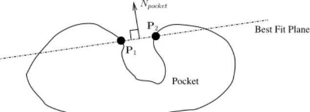
since a smaller e allows the probe easier access to the pocket. Npocket is com-puted by first finding the best fit plane for all mesh vertices between the pocket and its neighboring flat region (such as P1and P2in Fig. 6), then Npocketis simply the normal of the best fit plane, where the normal direction points away from the pocket. To justify the choice of emax as one control parameter, the rim (a non-planar 3D curve) of each large receptor pocket needs to be adequately represented by its best fit plane. The data in supplementary material indicate that the best fit planes are indeed good approximations of the rims. Both the mean and the stan-dard deviation of distances between all MSMS surface vertices that belong to the
rim of each large receptor pocket and its best fit plane are listed in supplementary material.
Best Fit Plane
Pocket P1
P2
Npocket
Figure 6: The pocket’s normal Npocketis determined by mesh vertices between the pocket and its neighboring flat region (such as P1 and P2).
In the second stage, rays are cast toward the probe in order to detect probe orientations for which protrusions are aligned with the receptor pocket. Suppose that a ray from the first stage detected a large pocket, its direction is reversed (i.e., let it travel in the direction of −Vray as shown in Fig. 5.b). If the first intersec-tion between the ray (after the reversion of the direcintersec-tion) and the probe surface occurs on a protrusion, the receptor pocket and the probe protrusion are consid-ered to be aligned. For example, the pocket/protrusion pair in Fig. 5 is aligned. As mentioned before, the second round of ray casting is repeated once for each orientation of the probe at that particular position.
Influence of h and e
max: Two-pass RCF filter
Both h and emax have a significant impact on the effectiveness and the efficiency of RCF. If h is too small, the pockets that are not located in the neighborhood of the axis passing through Pp and Pr may be missed. For example, the two
pocket/protrusion pairs in Fig. 7 will not be detected if h is set to a small value. On the other hand, if a large h is also used for all pockets that are located in the neighborhood of the axis (see Fig. 5), the filtering efficiency will decrease and this results in slower docking. emax has a similar effect. When emax is too small, a pocket may not be detected. But a large emax will lead to decreased filtering efficiency.
Pocket 2 Protrusion 1 Rays Protrusion 2
Pocket 1 Probe
Receptor
Pp
Pr
Figure 7: To detect the pockets that are not located in the neighborhood of the axis that passes through Ppand Pr, h must have a larger value.
Instead of a single-pass ray casting with a large h and a large emax, we propose a two-pass ray casting approach to dramatically improve the efficiency of the filter. The values of h and the cutoff angle emax for the two passes are given in Table I (see the Results and Discussion section for a short discussion on how the values of these parameters were chosen).
RCF works as follows: In the first pass, both h and emaxare set to small values. If some large pockets are not detected after the first pass, the values of both h and emax are increased and a second pass is executed in order to cover cases like the one shown in Fig. 7. The complete RCF method with the two-pass ray casting is
Table I: Setting of the two-pass ray casting for detection of aligned large receptor pocket/probe protrusion pairs.
Pass h The cutoff angle emaxin radians
1 0.10 //5
2 0.50 //4
sketched in Algorithm 1. In the algorithm, q(P, R) specifies the configuration of the probe as a rigid body (i.e., its position P and orientation R).
We have implemented RCF-ATTRACT by integrating RCF with ATTRACT [3]1. RCF-ATTRACT consists of two stages: (1) the filtering stage using RCF; (2) the docking stage using energy minimization. The main difference between AT-TRACT and RCF-ATAT-TRACT is that RCF-ATAT-TRACT tries to dock the proteins by performing energy minimizations from and only from the start configurations of the probe stored in Qgood (obtained by RCF as shown in Algorithm 1), while ATTRACT iterates through all start configurations of the probe and minimizes energy from each and every one of the configurations. Consequently, substantial speedup of the docking can be achieved if RCF is highly efficient and the size of the set Qgood is much smaller than the total number of probe configurations used by ATTRACT.
1The ATTRACT implementation in Fortran we used was provided to us by prof. Martin
Algorithm 1: Ray Casting Filter (RCF).
input : A set Ssettingof two pairs of (h, emax) as shown in Table I, a set P of probe positions, and a set R of
probe orientations;
output: A set of good probe configurations Qgood;
1 Qgood← /0;
2 Construct surface meshes of both the receptor and the probe;
3 Slarge← characterization of local geometries of the proteins’ surfaces;
4 S#large← Slarge;
5 foreach s∈ Ssettingdo
6 h← s.h (i.e., set h to the value of the element h stored in the pair s);
7 emax← s.emax(i.e., set emaxto the value of the element emaxstored in the pair s);
8 foreach P∈ P do
9 Cast rays from the neighborhood of P toward the receptor;
10 Spocket← detected large receptor pocket(s) (i.e., ∈ Slarge);
11 if Spocket%= /0 then
12 foreach R∈ R do
13 Reverse the rays in intersections toward the probe to look for protrusions;
14 if protrusion(s) detected then
15 Qgood= Qgood∪ q(P,R);
16 S#pocket← pockets in Spocketaligned with the protrusion(s);
17 S#large= S#large\ S#pocket;
18 if S#
large= /0 then
19 break;
Results and Discussion
In this section, we compare both the running times and the solutions of ATTRACT and RCF-ATTRACT. In addition, we present values of the parameters for the surface mesh construction and the visibility computation, and evaluate the effi-ciency of RCF for extracting of the good probe configurations. We have used the data set of [3], which consists of 18 bound-bound protein pairs (i.e., 16 enzyme-enzyme inhibitor pairs (2PTC, 2SIC, 2KAI, 1CHO, 1ACB, 1UGH, 1BRS, 1FSS, 1AVW, 2TEC, 2SNI, 1TGS, 1CGI, 1CSE, 1BTH, 1BRC), one antibody-antigen pair (1MLC), and one hormone-hormone receptor pair (3HHR)) and 15 unbound-unbound enzyme-enzyme inhibitor pairs (2PTN + 1BA7, 1BRA + 1AAP, 1A2P
+ 1A19, 2HNT + 6PTI, 1CHG + 1HPT, 5CHA + 2OVO, 1SCD + 1ACB, 2ACE + 1FSC, 2PTN + 1HPT, 1AKZ + 1UGI, 2PKA + 6PTI, 2PTN + 4PTI, 1SUP + 3SSI, 1SUP + 2CI2, 1THM + 2TEC). All experiments were performed on a SUN workstation with two 3.0GHz dual-core AMD Opteron processors and 8GB RAM, although all computations were executed using a single core.
ATTRACT versus RCF-ATTRACT
We compared the solutions of ATTRACT and RCF-ATTRACT for both bound-bound cases and unbound-bound-unbound-bound cases, followed by a comparison of their run-ning times.
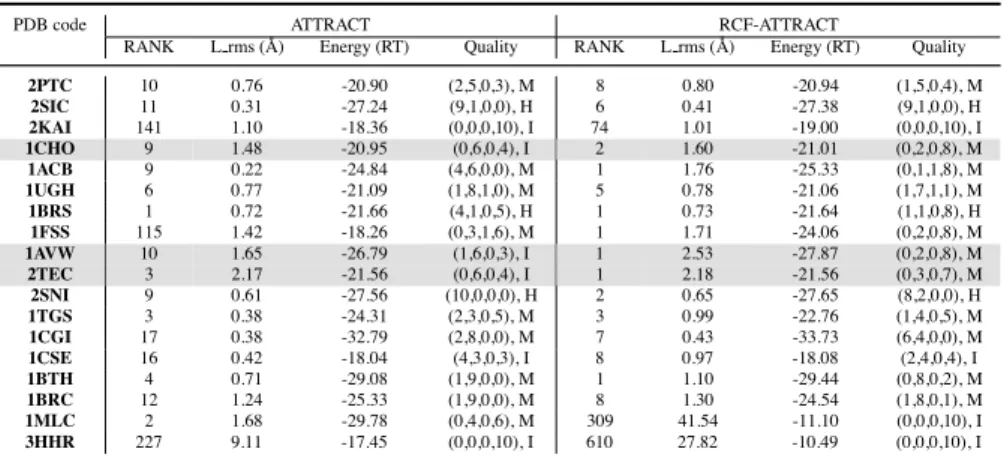
Using the default setting of h and emax, the solutions of ATTRACT and RCF-ATTRACT for the 18 bound-bound cases are listed in Table II. The 15 unbound-unbound cases are listed in Table III. The last complex in Table III (i.e., 1THM + 2TEC) is a special unbound-bound case. The L rms listed in the tables are the lowest RMSD of the backbone atoms of the ligand with respect to the experimen-tal complex structures (bound), along with the corresponding ranks and energies. The energy values are the ones computed with the reduced protein representation used by ATTRACT. When docking enzyme-enzyme inhibitor pairs, the solutions obtained by both methods are comparable both in terms of both energy and L rms values, but RCF-ATTRACT ranks these solutions with the lowest L rms higher than ATTRACT. For example, the native bound configuration of the 2TEC probe and the top-ranked configuration by RCF-ATTRACT are similar to each other, as shown in Fig. 8.a. The probe at both configurations blocks the active site
cav-ity of the enzyme. On the contrary, the top-ranked configuration by ATTRACT in Fig. 8.b does not block the active site cavity of the enzyme, even though it has a lower energy than both the native bound configuration and the top-ranked configuration by RCF-ATTRACT. For bound-bound cases, 6 lowest L rms solu-tions are ranked first by RCF-ATTRACT, while only 1 lowest L rms solution is ranked first by ATTRACT. For unbound-unbound cases, 3 lowest L rms solutions are ranked first by RCF-ATTRACT, while none is ranked first by ATTRACT. The RCF-ATTRACT failed to dock the antibody/antigen pair 1MLC. In addition to the aforementioned evaluation criteria, we used other CAPRI quality measures to rank docking predictions [34, 35]. Solutions are labelled as High, Medium, Ac-ceptable, and Incorrect depending on values of the fraction of native contacts ( fnat) and the backbone RMDS of the interface residues (I rms), in addition to L rms. The first element in the quality columns in Tables II and III is a quadruple of the numbers of solutions among the top 10/100 solutions (ranked by energy) that are labelled as High (H), Medium (M), Acceptable (A), and Incorrect (I) respectively. The second element of the Quality column in Table II is the classification of the quality of the top solution. In Table III, the second element is the rank of the first solution among the top 100 that are labelled as at least acceptable. The high-lighted rows in the two tables (3 for the bound-bound cases and 5 for the unbound-unbound cases) show enzyme-enzyme inhibitor pairs where the top-ranked solu-tions by RCF-ATTRACT are at least acceptable, whereas the top-ranked ones by ATTRACT are labelled as incorrect. Note that, for all cases in Table II and Ta-ble III where the lowest L rms solutions are ranked first by RCF-ATTRACT, these
solutions are at least of medium quality for the bound-bound cases (Table II) and of acceptable quality for the unbound-unbound cases (Table III). The quadruples in Table II and Table III show that ATTRACT in general produces more acceptable docking solutions among the top 10/100. Essentially, when docking with RCF-ATTRACT, there is a trade-off (as shown in supplementary material) between the docking speed and the numbers of high/medium/acceptable solutions, although not between the docking speed and the qualities of the top-ranked solutions. Table II: Comparison of the solutions of ATTRACT and RCF-ATTRACT for 18 bound-bound cases.
PDB code ATTRACT RCF-ATTRACT
RANK L rms ( ˚A) Energy (RT) Quality RANK L rms ( ˚A) Energy (RT) Quality
2PTC 10 0.76 -20.90 (2,5,0,3), M 8 0.80 -20.94 (1,5,0,4), M 2SIC 11 0.31 -27.24 (9,1,0,0), H 6 0.41 -27.38 (9,1,0,0), H 2KAI 141 1.10 -18.36 (0,0,0,10), I 74 1.01 -19.00 (0,0,0,10), I 1CHO 9 1.48 -20.95 (0,6,0,4), I 2 1.60 -21.01 (0,2,0,8), M 1ACB 9 0.22 -24.84 (4,6,0,0), M 1 1.76 -25.33 (0,1,1,8), M 1UGH 6 0.77 -21.09 (1,8,1,0), M 5 0.78 -21.06 (1,7,1,1), M 1BRS 1 0.72 -21.66 (4,1,0,5), H 1 0.73 -21.64 (1,1,0,8), H 1FSS 115 1.42 -18.26 (0,3,1,6), M 1 1.71 -24.06 (0,2,0,8), M 1AVW 10 1.65 -26.79 (1,6,0,3), I 1 2.53 -27.87 (0,2,0,8), M 2TEC 3 2.17 -21.56 (0,6,0,4), I 1 2.18 -21.56 (0,3,0,7), M 2SNI 9 0.61 -27.56 (10,0,0,0), H 2 0.65 -27.65 (8,2,0,0), H 1TGS 3 0.38 -24.31 (2,3,0,5), M 3 0.99 -22.76 (1,4,0,5), M 1CGI 17 0.38 -32.79 (2,8,0,0), M 7 0.43 -33.73 (6,4,0,0), M 1CSE 16 0.42 -18.04 (4,3,0,3), I 8 0.97 -18.08 (2,4,0,4), I 1BTH 4 0.71 -29.08 (1,9,0,0), M 1 1.10 -29.44 (0,8,0,2), M 1BRC 12 1.24 -25.33 (1,9,0,0), M 8 1.30 -24.54 (1,8,0,1), M 1MLC 2 1.68 -29.78 (0,4,0,6), M 309 41.54 -11.10 (0,0,0,10), I 3HHR 227 9.11 -17.45 (0,0,0,10), I 610 27.82 -10.49 (0,0,0,10), I
The running time of RCF-ATTRACT is the sum of following two terms: 1. T1: running time of RCF (i.e., computing surface meshes of both the
re-ceptor and the probe using MSMS and then dividing them into pockets, protrusions, and flat regions according to their visibilities, and then using the two-pass ray casting to find all aligned large receptor pocket/probe pro-trusion pairs in order to extract Qgood);
Table III: Comparison of the solutions of ATTRACT and RCF-ATTRACT for 15 unbound-unbound cases.
PDB code ATTRACT RCF-ATTRACT
RANK L rms ( ˚A) Energy (RT) Quality RANK L rms ( ˚A) Energy (RT) Quality
2PTN + 1BA7 45 6.55 -18.04 (0,4,23,73), 3 1 7.91 -20.42 (0,0,2,98), 1 1BRA + 1AAP 21 4.55 -19.54 (0,17,13,70), 2 9 4.60 -19.58 (0,12,14,74), 1 1A2P + 1A19 261 9.56 -14.12 (0,2,7,91), 11 23 9.59 -15.89 (0,3,5,92), 5 2HNT + 6PTI 2539 10.43 -11.31 (0,0,0,100), x 435 10.43 -10.78 (0,0,0,100), x 1CHG + 1HPT 1680 5.61 -11.55 (0,0,0,100), x 104 20.25 -11.58 (0,0,0,100), x 5CHA + 2OVO 2 8.95 -20.22 (0,9,4,87), 1 1 8.96 -20.26 (0,2,0,98), 1 1SCD + 1ACB 43 2.03 -16.27 (0,7,0,93), 14 18 2.13 -16.02 (0,5,2,93), 4 2ACE + 1FSC 810 3.08 -14.69 (0,0,0,100), x 77 4.64 -15.57 (0,3,9,88), 21 2PTN + 1HPT 351 3.05 -13.88 (0,0,6,94), 27 272 3.15 -10.42 (0,5,6,89), 3 1AKZ + 1UGI 1741 5.89 -11.49 (0,0,14,86), 1 391 6.98 -10.34 (0,0,12,88), 1 2PKA + 6PTI 747 4.47 -14.90 (0,0,2,98), 52 112 4.64 -16.57 (0,3,4,93), 19 2PTN + 4PTI 100 18.81 -15.36 (0,4,4,92), 3 32 18.90 -14.54 (0,2,2,96), 1 1SUP + 3SSI 5 5.20 -19.52 (0,7,6,87), 2 1 5.22 -19.77 (0,15,7,78), 1 1SUP + 2CI2 379 6.77 -12.94 (0,2,9,89), 25 109 6.75 -12.94 (0,1,9,90), 12 1THM + 2TEC 7 1.97 -19.02 (0,6,0,94), 5 32 2.31 -14.97 (0,12,3,85), 1 (a) (b)
Figure 8: The figure on the left shows the top-ranked 2TEC probe configuration by RCF-ATTRACT (in darker gray, L rms = 2.18 ˚A, and energy = −21.56RT), while the figure on the right shows the top-ranked 2TEC probe configuration by ATTRACT (in darker gray, L rms = 39.10 ˚A, and energy =−22.62RT). The native bound configurations of the 2TEC probe and the 2TEC receptor are shown in black and light gray, respectively, in both figures. The energy between the bound probe and the bound receptor is−12.55RT.
2. T2: computational time for docking the proteins using energy minimization
from configurations in Qgood.
As shown in Table IV, RCF-ATTRACT is in average 14.0 times faster than ATTRACT for bound-bound pairs. Among the enzyme-enzyme inhibitor pairs, RCF-ATTRACT needs less than 10 minutes to dock all pairs except 2KAI and less than 5 minutes for 8 pairs. When docking unbound-unbound protein pairs, the average speedup is 15.2 times as shown in Table V. RCF-ATTRACT needs less than 10 minutes to dock all pairs except two (i.e., 2ACE + 1FSC, 1SUP + 3SSI) and less than 5 minutes for 10 pairs.
Table IV: The comparison of the running times of ATTRACT and RCF-ATTRACT when docking bound-bound proteins.
Protein Data Bank code ATTRACT (min) RCF-ATTRACT (min) Speedup
T1 T2 - Ti 2PTC 50.2 0.3 5.0 5.3 9.5 2SIC 93.4 0.5 8.4 8.9 10.5 2KAI 48.7 1.6 9.0 10.6 4.6 1CHO 45.3 0.3 2.7 3.0 15.1 1ACB 55.6 0.4 5.2 5.6 9.9 1UGH 69.3 0.4 3.9 4.3 16.1 1BRS 42.5 0.7 7.2 7.9 5.4 1FSS 111.6 1.1 5.7 6.8 16.4 1AVW 136.7 0.4 6.2 6.6 20.7 2TEC 59.3 0.4 3.8 4.2 14.1 2SNI 62.0 0.4 4.5 4.9 12.7 1TGS 45.9 0.4 3.7 4.1 11.2 1CGI 49.2 0.4 5.0 5.4 9.1 1CSE 62.0 0.4 3.4 3.8 16.3 1BTH 58.1 0.5 3.6 4.1 14.2 1BRC 46.7 0.3 3.1 3.4 13.7 1MLC 214.8 0.9 5.1 6.0 35.8 3HHR 421.3 1.3 22.8 24.1 17.5 Average 92.9 0.6 6.0 6.6 14.0
By eliminating start configurations that are not likely to result in configura-tions similar to the correct bound configuration after energy minimizaconfigura-tions, RCF enables much faster docking. In addition, the lowest L rms solutions obtained by
Table V: The comparison of the running times of ATTRACT and RCF-ATTRACT when docking unbound-unbound proteins.
Protein Data Bank code ATTRACT (min) RCF-ATTRACT (min) Speedup
T1 T2 - Ti 2PTN + 1BA7 133.0 0.4 4.1 4.5 29.6 1BRA + 1AAP 46.2 0.4 5.1 5.5 8.4 1A2P + 1A19 43.6 0.7 4.0 4.7 9.3 2HNT + 6PTI 54.2 0.5 2.8 3.3 16.4 1CHG + 1HPT 46.5 0.4 1.5 1.9 24.5 5CHA + 2OVO 47.6 0.4 3.9 4.3 11.1 1SCD + 1ACB 58.9 0.4 5.5 5.9 10.0 2ACE + 1FSC 107.5 1.1 9.3 10.4 10.3 2PTN + 1HPT 45.0 0.3 1.9 2.2 20.5 1AKZ + 1UGI 68.1 0.5 3.5 4.0 17.0 2PKA + 6PTI 48.4 0.4 3.0 3.4 14.2 2PTN + 4PTI 47.8 0.3 1.7 2.0 23.9 1SUP + 3SSI 93.1 0.6 9.9 10.5 8.9 1SUP + 2CI2 60.0 0.5 6.9 7.4 8.1 1THM + 2TEC 59.5 0.4 3.4 3.8 15.7 Average 64.0 0.5 4.3 4.9 15.2
RCF-ATTRACT are comparable (in terms of both energy and L rms) to the ones obtained by ATTRACT, but RCF-ATTRACT ranks these solutions higher. How-ever, RCF-ATTRACT failed to dock the antibody-antigen pair (1MLC), because the current implementation of RCF focuses on docking between a large pocket and a protrusion, which is common in enzyme-enzyme inhibitor complexes [36], even though the docking interfaces between antibody-antigen complexes are pla-nar [37]. Nevertheless, since there is a high degree of shape complementarity between the antibody-antigen interfaces, we were able to dock 1MLC success-fully and obtained an L rms of the top-ranked solution of 1.71 ˚A, when we used a slightly different implementation of RCF to find matching between small re-ceptor pockets (i.e., the pockets that are part of Ssmall) and probe protrusions. In essence, we replaced Slarge in Algorithm 1 with Ssmall in order to find all probe configurations that align at least one probe protrusion with one small receptor
pocket in Ssmall. Finally, both ATTRACT and RCF-ATTRACT failed to dock the hormone-hormone receptor pair (3HHR), and hence it seems that the scoring function in ATTRACT should be improved/refined for hormone-hormone receptor complexes.
Parameter setting
We present first values of the parameters for the surface mesh construction and the visibility computation, followed by evaluating of the efficiency of RCF and demonstration of why the two passes in RCF are indeed necessary. At the end of this subsection, we evaluate the choices of the RCF parameters.
A surface mesh is computed by rolling a probe sphere with a radius of 1.5 ˚A over a protein and then triangulating the obtained surface with a vertex density of 1.0vertex/ ˚A2, where the values of the probe sphere radius and the vertex density are the default values in MSMS [26, 27]. In order to divide the surface mesh into pockets, protrusions, and flat regions, we set the number of rays we cast for each vertex to 100 (i.e., n = 100).
Since all pockets in Slargecan be reliably detected with the setting of pass 2 in Table I, it was possible to use this setting and run a single-pass ray casting. How-ever, as shown in Table VI, ratios of npoor to ntotal (i.e., the filtering power) are significantly lower when the single-pass ray casting is applied instead of the two-pass ray casting, where npoorand ntotalrepresent the number of poor probe config-urations and the number of all probe configconfig-urations, respectively. Consequently, the single-pass ray casting will lead to much longer docking times, because the
time saved from systematic docking methods increases linearly with the ratio of
npoor to ntotal. Although it is possible to have more than two passes to allow h and emaxto be adjusted gradually, the data show in Table VI that the first pass, the one with the most restrictive setting, is enough for a majority of the protein pairs and a second pass is rarely used.
Table VI: Ratios of npoor to ntotal are significantly higher when the two-pass ray casting is applied instead of the single-pass ray casting. The number of aligned pockets over the total number of large pockets is indicated in each pair of paren-theses.
npoor/ntotal
Protein Data Bank code Two Pass Ray Casting One Pass Ray Casting Pass 1 Pass 2 2PTC 0.91 (4/4) 0.61 (4/4) 2SIC 0.92 (2/2) 0.71 (2/2) 2KAI 0.94 (2/3) 0.83 (3/3) 0.61 (3/3) 1CHO 0.94 (4/4) 0.48 (4/4) 1ACB 0.90 (5/5) 0.35 (5/5) 1UGH 0.95 (1/1) 0.89 (1/1) 1BRS 0.97 (2/4) 0.81 (4/4) 0.59 (4/4) 1FSS 0.95 (1/1) 0.83 (1/1) 1AVW 0.96 (3/3) 0.59 (3/3) 2TEC 0.94 (2/2) 0.75 (2/2) 2SNI 0.94 (1/1) 0.85 (1/1) 1TGS 0.93 (2/2) 0.72 (2/2) 1CGI 0.90 (4/4) 0.44 (4/4) 1CSE 0.96 (1/1) 0.86 (1/1) 1BTH 0.93 (1/1) 0.85 (1/1) 1BRC 0.94 (3/3) 0.65 (3/3) 1MLC 0.98 (1/1) 0.87 (1/1) 3HHR 0.95 (1/1) 0.88 (1/1)
Next, we evaluated the impact of the two RCF thresholds (i.e., pminand pmax) on the solutions generated by RCF-ATTRACT. The solutions for 16 bound-bound enzyme-enzyme inhibitor pair cases when (1) pmax= 0.65, pmin= 0.30; (2) pmax= 0.85, pmin= 0.50 are shown in Table VII. The solutions obtained when pmax = 0.75, pmin= 0.40 (i.e., the default setting) are shown in Table II. The results show that RCF-ATTRACT is quite robust with respect to the choices of both pmin and
exceptions to this are when the lowest L rms is 7.98 ˚A for 1FSS when pmax= 0.65,
pmin= 0.30; the lowest L rms is 15.11 ˚A for 1CSE when pmax= 0.85, pmin= 0.50. For both cases, the top-ranked solutions are labelled as incorrect according to the CAPRI criteria. The L rms of the top 10 solutions in Table II and Table VII are displayed in box and whisker diagrams in supplementary material. Table II shows only the 16 bound-bound enzyme-enzyme inhibitor pairs. Results tend to show that using smaller receptor pocket patches in terms of area compared to the patches detected using the default values for pmin and pmax for docking is more harmful than using smaller probe protrusion patches, because three top-ranked solutions are labelled as incorrect when pmax = 0.65, pmin= 0.30, while four top-ranked solutions are labelled as incorrect when pmax = 0.85, pmin= 0.50.
Table VII: Comparison of the solutions of RCF-ATTRACT for 16 bound-bound enzyme-enzyme inhibitor pairs cases when (1) pmax = 0.65, pmin= 0.30; (2)pmax = 0.85, pmin= 0.50.
Protein Data Bank code RCF-ATTRACT(1) RCF-ATTRACT(2)
RANK L rms ( ˚A) Energy (RT) Quality RANK L rms ( ˚A) Energy (RT) Quality
2PTC 3 1.53 -22.47 (0,5,0,5), M 8 0.76 -20.92 (2,5,0,3), M 2SIC 1 0.43 -27.42 (5,3,0,2), H 6 0.68 -27.26 (6,0,1,3), H 2KAI 50 0.83 -18.49 (0,0,0,10), I 48 0.64 -19.09 (0,0,0,10), I 1CHO 2 1.57 -21.00 (0,3,0,7), M 2 1.69 -21.32 (0,2,0,8), M 1ACB 5 0.34 -24.20 (3,3,1,3), M 9 0.18 -24.37 (6,4,0,0), M 1UGH 3 1.21 -19.90 (0,3,1,6), M 6 0.77 -20.47 (1,7,1,1), M 1BRS 1 0.72 -21.66 (1,0,0,9), H 2 0.72 -21.15 (2,2,0,6), H 1FSS 78 7.98 -12.30 (0,0,0,10), I 3 1.62 -23.72 (0,2,1,7), M 1AVW 2 2.43 -27.88 (0,1,0,9), I 5 2.12 -25.99 (0,7,0,3), I 2TEC 1 2.14 -21.50 (0,3,0,7), M 2 2.14 -21.50 (0,5,0,5), I 2SNI 4 0.65 -27.58 (8,2,0,0), H 3 0.64 -27.52 (7,0,0,3), H 1TGS 3 1.16 -24.99 (0,6,0,4), M 5 0.31 -23.63 (2,5,0,3), M 1CGI 5 0.42 -33.73 (6,4,0,0), M 15 0.37 -33.15 (1,9,0,0), M 1CSE 8 0.94 -17.50 (3,2,0,5), M 23 15.11 -14.03 (0,0,0,10), I 1BTH 1 0.84 -29.62 (1,4,0,5), H 3 0.70 -29.06 (3,0,0,7), H 1BRC 11 1.30 -24.48 (0,10,0,0), M 16 1.24 -25.29 (0,10,0,0), M
The values of h and emax for the first pass given in Table I were chosen by comparing the solutions of ATTRACT and RCF-ATTRACT for 9 different
combi-nations of h and emaxshown in Table VIII, where the default setting is highlighted. Note that only the settings of the first pass are shown in Table VIII, because the settings of the second pass (as shown in Table I) do not change. The solutions of ATTRACT and RCF-ATTRACT for the 18 bound-bound cases and the 9 settings in Table VIII are listed in Table IX, and the solutions corresponding to the default setting are highlighted. The three values in each cell represent (1) the rank of the solution with the lowest L rms with respect to the experimental complex structure, (2) the L rms value ( ˚A) of the solution, and (3) the energy (RT) of the solution. Although the running times of both methods are not shown for improved read-ability of Table IX, the data indicate that RCF-ATTRACT is faster and thus more efficient when h = 0.10 (i.e., settings S1, S4, and S7) than when both h = 0.15 and
h = 0.20. This is achieved without sacrificing the docking quality (at least for set-tings S1 and S4). Setting S4consistently results in faster docking than setting S1.
For most cases, setting S7results in even faster docking, but worse solutions for
some protein pairs (e.g., 1FSS). Consequently, setting S4was chosen as the default
setting and the values of this setting are shown in Table I. Furthermore, the data in the table demonstrate that the choices of the RCF parameters h and emaxhave little effect on the results obtained by RCF-ATTRACT, because the solutions obtained by ATTRACT and RCF-ATTRACT (using 9 different settings) are comparable in terms of both energy and L rms, and in general RCF-ATTRACT ranks these so-lutions with the lowest L rms higher than ATTRACT, at least for enzyme-enzyme inhibitor pairs.
Table VIII: Different settings of the first pass of the two-pass ray casting for de-tection of aligned large receptor pocket/probe protrusion pairs.
Setting Pass 1 h emax S1 0.10 //4 S2 0.15 //4 S3 0.20 //4 S4 0.10 //5 S5 0.15 //5 S6 0.20 //5 S7 0.10 //6 S8 0.15 //6 S9 0.20 //6
Conclusions
We have presented a novel and efficient filtering method called Ray Casting Filter (RCF)2that significantly speeds up protein-protein docking compared to system-atic docking methods. This method finds aligned receptor pocket/probe protru-sion pairs without explicit similarity computations. The RCF method enables the integration of local shape feature matching into systematic docking methods. Fur-thermore, we tested RCF with ATTRACT on both the bound-bound cases and the unbound-unbound cases of [3] to verify its efficiency and accuracy. Our results in-dicate the lowest L rms solutions resulting from RCF-ATTRACT and ATTRACT are comparable in terms of both energy and L rms for enzyme-enzyme inhibitor complexes, but RCF-ATTRACT ranks these solutions higher. Note that RCF can also be integrated with other systematic methods. For examples, by integrating a variant of RCF with the FFT-based methods, many poor orientations of the probe could be eliminated, thus enabling faster docking.
The focus of this paper is on enzyme-enzyme inhibitor complexes. Conse-quently, one possible improvement to the RCF would be to look for large planar surface/large planar surface pairs, so that antibody-antigen complexes can also be docked successfully. Another area of future investigation consists of optimizing the parameter settings using a learning stage based on a large set of benchmark docking pairs. Finally, we plan in the future to dock unbound proteins by introduc-ing flexibility (first flexible side-chains, followed by flexible loops). One idea that we are currently investigating is to prune off parts of solvent exposed side-chains on the unbound proteins (as proposed in [3]) and then produce docked complexes of such simplified models using RCF-ATTRACT. After this we can apply a recent algorithm called transition-based RRT (T-RRT) [38] to refine the candidate con-formations while considering side-chain flexibility. The interest of T-RRT with re-spect to a simple energy minimization procedure is that the conformational search is less local, therefore enabling us to find low-energy conformations behind local energy barriers.
Acknowledgments
We would like to thank prof. Martin Zacharias, Physik-Department, Technis-che Universit¨at M¨unTechnis-chen, for providing us with his ATTRACT implementation in Fortran, and for his helpful discussions and advice. We are also very grateful to
Table IX: The solutions of ATTRACT and RCF-ATTRACT for the 18 bound-bound cases and the 9 settings in Table VIII.
RCF-ATTRACT PDB Code ATTRACT S1 S2 S3 S4 S5 S6 S7 S8 S9 2PTC 10 11 11 9 8 8 6 6 9 9 0.76 0.80 0.79 0.79 0.80 0.79 0.79 0.82 0.89 1.01 -20.90 -20.94 -20.95 -20.95 -20.94 -20.95 -20.95 -21.25 -21.21 -20.69 2SIC 11 7 5 6 6 4 4 3 4 7 0.31 0.39 0.40 0.36 0.41 0.39 0.39 0.40 0.50 0.40 -27.24 -27.44 -27.43 -27.44 -27.38 -27.43 -27.53 -27.42 -27.32 -27.41 2KAI 141 64 55 86 74 66 56 77 103 63 1.10 0.82 0.68 0.81 1.01 0.85 0.63 1.01 0.95 0.63 -18.36 -18.50 -19.14 -18.50 -19.00 -19.15 -19.09 -19.00 -18.33 -19.09 1CHO 9 2 3 4 2 3 4 5 4 5 1.48 1.60 1.57 1.58 1.60 1.57 1.58 1.58 1.58 1.58 -20.95 -21.01 -21.00 -21.00 -21.01 -21.00 -21.00 -21.00 -21.00 -21.00 1ACB 9 3 5 8 1 4 7 12 2 5 0.22 0.34 0.23 0.36 1.76 0.39 0.35 0.16 0.39 0.47 -24.84 -24.21 -24.84 -24.24 -25.33 -24.37 -24.03 -24.36 -24.37 -24.66 1UGH 6 5 4 7 5 7 2 10 8 4 0.77 0.82 0.77 0.79 0.78 1.25 1.73 1.56 0.75 0.77 -21.09 -20.46 -21.07 -20.46 -21.06 -20.10 -22.28 -18.37 -20.49 -21.09 1BRS 1 1 1 1 1 5 1 1 2 1 0.72 0.73 0.73 0.72 0.73 0.67 0.72 0.73 0.72 0.72 -21.66 -21.64 -21.66 -21.66 -21.64 -19.48 -21.66 -21.64 -21.65 -21.66 1FSS 115 5 3 24 1 1 1 9 1 1 1.42 1.60 1.63 1.19 1.71 1.80 1.79 9.07 1.79 1.79 -18.26 -22.44 -23.89 -18.64 -24.06 -24.04 -24.05 -18.34 -24.05 -24.05 1AVW 10 2 4 2 1 1 3 1 2 3 1.65 1.84 1.22 1.60 2.53 2.53 1.99 2.42 2.44 1.12 -26.79 -28.82 -27.57 -28.71 -27.87 -27.88 -28.55 -27.81 -27.88 -27.21 2TEC 3 1 2 1 1 1 1 1 1 1 2.17 2.18 1.96 2.18 2.18 2.15 2.18 2.15 2.23 2.18 -21.56 -21.56 -21.49 -21.55 -21.56 -21.46 -21.55 -21.46 -21.28 -21.55 2SNI 9 6 2 3 2 6 3 3 3 6 0.61 0.71 0.63 0.64 0.65 0.64 0.65 0.64 0.65 0.64 -27.56 -27.48 -27.66 -27.65 -27.65 -27.51 -27.50 -27.65 -27.50 -27.50 1TGS 3 2 3 2 3 2 4 2 2 4 0.38 1.19 0.77 0.32 0.99 1.21 1.16 1.19 1.14 0.57 -24.31 -25.02 -24.77 -24.11 -22.76 -25.00 -24.38 -25.02 -25.22 -24.20 1CGI 17 8 10 9 7 9 11 5 7 11 0.38 0.38 0.44 0.43 0.43 0.44 0.37 0.43 0.43 0.37 -32.79 -33.33 -33.74 -33.73 -33.73 -33.74 -33.14 -33.83 -33.72 -33.14 1CSE 16 11 6 6 8 5 6 8 4 3 0.42 0.97 0.96 0.99 0.97 0.96 1.06 0.97 0.96 1.08 -18.04 -18.08 -19.27 -19.40 -18.08 -19.27 -19.01 -18.08 -19.27 -19.42 1BTH 4 2 3 1 1 3 2 2 3 1 0.71 0.98 1.08 0.69 1.10 1.03 0.71 1.11 0.71 0.87 -29.08 -29.54 -29.25 -29.51 -29.44 -29.36 -29.54 -29.10 -29.54 -29.64 1BRC 12 9 7 5 8 8 10 6 6 5 1.24 1.19 1.27 1.24 1.30 1.27 1.46 1.31 1.27 1.35 -25.33 -24.97 -25.41 -25.32 -24.54 -25.35 -24.55 -25.25 -25.35 -25.41 1MLC 2 664 1207 68 309 944 20 40 244 288 1.68 42.14 42.29 24.68 41.54 43.24 24.90 49.56 45.39 45.33 -29.78 -11.08 -10.95 -17.20 -11.10 -10.21 -19.26 -14.13 -13.11 -13.40 3HHR 227 16 164 1 610 398 8 103 10 274 9.11 22.79 19.97 49.37 27.82 25.85 17.80 22.68 26.40 23.91 -17.45 -18.30 -14.42 -31.43 -10.49 -11.74 -19.57 -13.08 -17.23 -12.05
Bibliography
[1] I. S. Moreira, P. A. Fernandes, and M. J. Ramos, “Protein-protein docking dealing with the unknown,” Journal of Computational Chemistry, vol. 31, pp. 317–342, Jan. 2010.
[2] N. Andrusier, E. Mashiach, R. Nussinov, and H. J. Wolfson, “Principles of flexible protein-protein docking,” Proteins: Structure, Function, and
Bioin-formatics, vol. 73, pp. 271–289, Nov. 2008.
[3] M. Zacharias, “Protein-protein docking with a reduced protein model ac-counting for side-chain flexibility,” Protein Science, vol. 12, pp. 1271–1282, June 2003.
[4] S. J. de Vries, A. D. J. van Dijk, M. Krzeminski, M. van Dijk, A. Thureau, V. Hsu, T. Wassenaar, and A. M. J. J. Bonvin, “Haddock versus haddock: New features and performance of haddock2.0 on the capri targets,” Proteins:
[5] M. Kr´ol, R. A. Chaleil, A. L. Tournier, and P. A. Bates, “Implicit flexibility in protein docking: Cross-docking and local refinement,” Proteins: Structure,
Function, and Bioinformatics, vol. 69, pp. 750–757, Dec. 2007.
[6] J. Cherfils and J. Janin, “Protein docking algorithms: simulating molecular recognition,” Current Opinion in Structural Biology, vol. 3, pp. 265–269, 1993.
[7] G. R. Smith and M. J. E. Sternberg, “Prediction of protein–protein interac-tions by docking methods,” Current Opinion in Structural Biology, vol. 12, pp. 28–35, Feb. 2002.
[8] C. J. Camacho and S. Vajda, “Protein–protein association kinetics and pro-tein docking,” Current Opinion in Structural Biology, vol. 12, pp. 36–40, Feb. 2002.
[9] I. Halperin, B. Ma, H. Wolfson, and R. Nussinov, “Principles of docking: An overview of search algorithms and a guide to scoring functions,” Proteins:
Structure, Function, and Genetics, vol. 47, pp. 409–443, June 2002.
[10] I. D. Kuntz, J. M. Blaney, S. J. Oatley, R. Langridge, and T. E. Ferrin, “A ge-ometric approach to macromolecule-ligand interactions,” Journal of
Molec-ular Biology, vol. 161, pp. 269–288, Oct. 1982.
[11] M. L. Connolly, “Shape complementarity at the hemoglobin _1`1 subunit
[12] P. H. Walls and M. J. E. Sternberg, “New algorithm to model protein-protein recognition based on surface complementarity: Applications to antibody-antigen docking,” Journal of Molecular Biology, vol. 228, pp. 277–297, Nov. 1992.
[13] R. Norel, S. L. Lin, H. J. Wolfson, and R. Nussinov, “Shape complementar-ity at protein-protein interfaces,” Biopolymers, vol. 34, no. 7, pp. 933–940, 1994.
[14] R. Norel, S. L. Lin, H. J. Wolfson, and R. Nussinov, “Molecular surface com-plementarity at protein-protein interfaces: the critical role played by surface normals at well placed, sparse, points in docking,” Journal of Molecular
Biology, vol. 252, no. 2, pp. 263–273, 1995.
[15] T. J. Ewing, S. Makino, A. G. Skillman, and I. D. Kuntz, “Dock 4.0: search strategies for automated molecular docking of flexible molecule databases,”
J Comput Aided Mol Des, vol. 15, pp. 411–428, May 2001.
[16] B. Sandak, H. J. Wolfson, and R. Nussinov, “Flexible docking allowing in-duced fit in proteins: insights from an open to closed conformational iso-mers,” Proteins: Structure, Function, and Genetics, vol. 32, pp. 159–174, Aug. 1998.
[17] D. Duhovny, R. Nussinov, and H. J. Wolfson, “Efficient unbound docking of rigid molecules,” in Proceedings of the Second International Workshop
on Algorithms in Bioinformatics, vol. 2452 of Lecture Notes In Computer Science, pp. 185–200, 2002.
[18] F. Cazals, F. Proust, R. P. Bahadur, and J. Janin, “Revisiting the voronoi description of protein-protein interfaces,” Protein Science, vol. 15, pp. 2082– 2092, Sept. 2006.
[19] E. Katchalski-Katzir, I. Shariv, M. Eisenstein, A. A. Friesem, C. Aflalo, and I. A. Vakser, “Molecular surface recognition: determination of geometric fit between proteins and their ligands by correlation techniques,” in
Proceed-ings of the National Academy of Sciences of the United States of America,
vol. 89, pp. 2195–2199, 1992.
[20] M. Meyer, P. Wilson, and D. Schomburg, “Hydrogen bonding and molecular surface shape complementarity as a basis for protein docking,” Journal of
Molecular Biology, vol. 264, pp. 199–210, Nov. 1996.
[21] H. A. Gabb, R. M. Jackson, and M. J. E. Sternberg, “Modelling protein docking using shape complementarity, electrostatics and biochemical infor-mation,” Journal of Molecular Biology, vol. 272, pp. 106–120, Sept. 1997. [22] D. W. Ritchie and G. J. L. Kemp, “Protein docking using spherical polar
fourier correlations,” Proteins: Structure, Function, and Genetics, vol. 39, pp. 178–194, May 2000.
[23] R. Chen and Z. Weng, “Docking unbound proteins using shape complemen-tarity, desolvation, and electrostatics,” Proteins: Structure, Function and
Ge-netics, vol. 47, no. 3, pp. 281–294, 2002.
[24] S. D. Roth, “Ray casting for modeling solids,” Computer Graphics and
Im-age Processing, vol. 18, pp. 109–144, Feb. 1982.
[25] B. Li, S. Turuvekere, M. Agrawal, D. La, K. Ramani, and D. Kihara, “Char-acterization of local geometry of protein surfaces with the visibility crite-rion,” Proteins: Structure, Function, and Bioinformatics, vol. 71, no. 2, pp. 670–683, 2008.
[26] M. F. Sanner, “Fast and robust computation of molecular surfaces,” in
Pro-ceedings of the eleventh annual symposium on Computational geometry,
pp. 406–407, 1995.
[27] M. F. Sanner and A. J. Olson, “Reduced surface - an efficient way to compute molecular surfaces,” Biopolymers, vol. 38, no. 3, pp. 305–320, 1996.
[28] A. Yershova, S. Jain, S. M. LaValle, and J. C. Mitchell, “Generating uniform incremental grids on SO(3) using the hopf fibration,” International Journal
of Robotics Research, vol. 29, pp. 801–812, June 2010.
[29] S. Gottschalk, M. C. Lin, and D. Manocha, “OBB-Tree: A hierarchical struc-ture for rapid interference detection,” in Proc. of ACM SIGGRAPH, pp. 171– 180, 1996.
[30] E. Larsen, S. Gottschalk, M. C. Lin, and D. Manocha, “Fast proximity queries with swept sphere volumes,” in Proc. of Int. Conf. on Robotics and
Automation, pp. 3719–3726, 2000.
[31] F. Cazals, F. Chazal, and T. Lewiner, “Molecular shape analysis based upon the morse-smale complex and the connolly function,” in Proc. of the
nine-teenth annual symposium on Computational geometry, SCG ’03, pp. 351–
360, 2003.
[32] P. K. Agarwal, H. Edelsbrunner, J. Harer, and Y. S. Wang, “Extreme el-evation on a 2-manifold,” in Proc. of the twentieth annual symposium on
Computational geometry, SCG ’04, pp. 357–365, 2004.
[33] L.-P. Albou, B. Schwarz, O. Poch, J. M. Wurtz, and D. Moras, “Defining and characterizing protein surface using alpha shapes,” Proteins: Structure,
Function, and Bioinformatics, vol. 76, pp. 1–12, 2009.
[34] R. M´endez, R. Leplae, L. De Maria, and S. J. Wodak, “Assessment of blind predictions of protein-protein interactions: current status of docking methods,” Proteins: Structure, Function, and Bioinformatics, vol. 52, no. 1, pp. 51–67, 2003.
[35] R. M´endez, R. Leplae, M. F. Lensink, and S. J. Wodak, “Assessment of capri predictions in rounds 3-5 shows progress in docking procedures,” Proteins:
[36] H. X. Lei and Y. Duan, “Incorporating intermolecular distance into protein-protein docking,” Protein Engineering, Design and Selection, vol. 17, no. 12, pp. 837–845, 2004.
[37] D. M. Webster, A. H. Henry, and A. R. Rees, “Antibody-antigen interac-tions,” Current Opinion in Structural Biology, vol. 4, no. 1, pp. 123–129, 1994.
[38] L. Jaillet, J. Cort´es, and T. Sim´eon, “Sampling-based path planning on configuration-space costmaps,” IEEE Transactions on Robotics, vol. 26, no. 4, pp. 635–646, 2010.