Quadratic distance methods applied to generalized normal Laplace distribution

Université de Montréal

Quadratic Distance Methods Applied to

Generalized Normal Laplace Distribution

par

Ionica Groparu-Cojocaru

Département de mathématiques et de statistique Faculté des arts et des sciences

Mémoire présenté à la Faculté des études supérieures en vue de l’obtention du grade de

lVlaître ès sciences (IVI.Sc.) en mathématiques

Orientation actuariat

mars 2007

p

C

D

de Montréal

Direction des bibtïothèques

AVIS

L’auteur a autorisé l’Université de Montréal à reproduire et diffuser, en totalité ou en partie, par quelque moyen que ce soit et sur quelque support que ce soit, et exclusivement à des fins non lucratives d’enseignement et de recherche, des copies de ce mémoire ou de cette thèse.

L’auteur et les coauteurs le cas échéant conservent la propriété du droit d’auteur et des droits moraux qui protègent ce document. Ni la thèse ou le mémoire, ni des extraits substantiels de ce document, ne doivent être imprimés ou autrement reproduits sans l’autorisation de l’auteur.

Afin de se conformer à la Loi canadienne sur la protection des renseignements personnels, quelques formulaires secondaires, coordonnées ou signatures intégrées au texte ont pu être enlevés de ce document. Bien que cela ait pu affecter la pagination, il n’y a aucun contenu manquant.

NOTICE

The author of this thesis or dissertation has granted a nonexciusive license allowing Université de Montréal to reproduce and publish the document, in part or in whole, and in any format, solely for noncommercial educationat and research purposes.

The author and co-authors if applicable retain copyright ownership and moral rights in this document. Neither the whole thesis or dissertation, flot substantial extracts from it, may be printed or otherwise reproduced without the author’s permission.

In compliance with the Canadian Privacy Act some supporting forms, contact information or signatures may have been removed from the document. While this may affect the document page count, it does flot represent any loss of content from the document.

faculté des études supérieures

Ce mémoire intitulé

Quadratic Distance Methods Applied to

Generalized Normal Laplace Distribution

présenté par

Ionica Groparu-Cojocaru

a été évalué par un jury composé des personnes suivantes Martin Goldstein (président-rapporteur) Louis G. Doray (directeur de recherche) Charles Dugas (membre du jury)

SOMMAIRE

Le but de cette thèse est d’analyser la méthode d’estimation des paramètres de la distribution normale généralisée de Laplace (GNL).

Nous proposons une méthode alternative pour estimer les paramètres basée sur la minimisation de la distance quaciratique entre les parties réelle et imaginaire des fonctions caractéristiques empiriques et théoriques.

L’estimateur de distance quaciratique (QDE) obtenu est convergent, robuste, asymptotiquernent sans biais et de distribution normale. On développe des statis tiques pour les tests d’ajustement et nous démontrons que les tests suivent asymp totiquement une distribution chi-carré.

Les résultats de la simulation sont fournis et les propriétés asymptotiques des estiinateurs obtenus sont étudiées.

$UMMARY

The purpose of this thesis is to analyze the methoci of parameter estimation of the generalized normal Laplace distribution (GNL).

We propose an alternative method for estimating the parameters based on mini

mizing the quadratic distance hetween the real and irnaginary parts of empirical and theoretical characteristic functions.

We show that the quadratic distance estirnator (QDE) ohtained is consistent, robust, asymptotically unbiased and normally distrihuted. We develop test sta tistics for goodness-of-fit and prove that these tests follow asymptotically a chi square distribution.

Simulation resuits are provideci and asymptotic properties of the estimators oh tained are studied.

Keywords: Empirical characteristic function, normal Laplace distribution, generalized normal Laplace distribution, quadratic distance estirnator, influence function, robustness, goodness-of-fit tests, simple anci composite hypotheses.

CONTENTS

Sommaire iii Summary iv List of tables vi Acknowledgements 1 Introduction 2

Chapter 1. The generalized normal Laplace distribution 4

1. 1. iViornent generating function anci

characteristic function ₅

1.2. Genesis, properties and financial applications of the

NL and GNL distributions 13

1.3. Estimation 23

Chapter 2. Quadratic transform distance estimators 26

2.1. Definition 27

2.2. Consistency and asymptotic norniality of the

quaciratic distance estimator 2$ 2.3. Influence functions for the quadratic distance

estimators 31

2.4. Goodness of fit tests 34

2.4.2. _{Gooclness of fit for the simple hypothesis}

. 35

2.4.3. _{Goodness of fit for the composite hypothesis}

36

Chapter 3. _{Inference for the parameters of the GNL distribution} using quadratic distance method ₃₈

3.1. _{Empirical characteristic fiinction}

and its properties ₃₉

3.2. _{Qnadratic distance estimator based on the characteristic ftmction of}

the GNL distribution ₄₆

3.3. _{Consistency arici asymiptotic norrnalit.y}

47

3.4. _{Robustmiess of the qua.clratic distance estimator based on the empirical}

characteristic function ₅₁ 3.5. Hypothesis testing 52 3.5.1. Simple hypothesis ₅₂ 3.5.2. Composite hypothesis 52

Chapter 4. Numerical illustrations ₅₄

4.1. Simulation resuits ₅₄

Chapter 5. Conclusion ₆₁

Bibliography

LI$T 0F TABLES

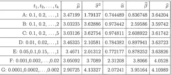
4.1 _{Estimatecl values of the QDE with Q(9) = I usiug a sample of size 500 55} 4.2 _{Estimateci values of the QDE with Q(O) I using a sample of size}

1000 ₅₆

4.3 _{Estirnateci values of the QDE with Q(O) = I using a sample of size}

10000 ₅₆

4.4 _{Absolute biases of the QDE with Q(O) = I using a sample of size 500} 57 4.5 _{Absolute biases of the QDE with Q(9) = I ushig a sample of size 1000 57} 4.6 _{Absolute biases of the QDE with}

_Q(&)

= I using a saniple of size 10000 58

4.7 _{Estirnated values of the QDE with}

_Q(&)

= Z() (size 500) 59

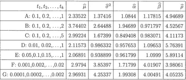
4.8 _{Estimateci values of the QDE with}

_Q(O)

_{= Z’(9) (size 1000)}

59 4.9 _{Estimated values of the QDE with Q(O) = ‘(6) (size 10000)}

59

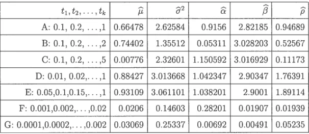
4.10 _{Estimatecl standard deviation (size 500)}

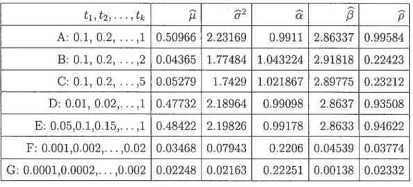
60 4.11 _{Estirnat.ed standard cleviatioii (size 1000)}

60 4.12 _{Estirnated standard cleviation (size 10000)}

ACKNOWLEDGEMENT$

I express my entire gratitude to my supervisor Prof. Louis G. Doray who offerecÏ

an insightful guiclance towards the progress of my project ancÏ who supervised this work with professionalisïn, interest and steacly encouragements.

I acknowledge the ongoing support received from Prof. Roch Roy auJ Prof. Marlène Frigon. I am also grateful to the professors from the Department of Mathematics anci Statistics for their scientific auJ valuable lectures.

I greatly benefited from the help provided by the informatics counselor Francis Forget auJ I would like to thank him.

For financial support, I woulcÏ like to acknowledge FQRNT, the Mathematics auJ Statistics Department, Fondation J.A. Bombardier auJ my supervisor Prof. Louis Doray.

Although the normal (Gaussian) distribution plays a central foie in basic statis tics, it has long been recognized that the empirical distributions of many plie nomena modelleci by the normal distribution sometimes do not follow closely to the Gaussian shape.

In recent years the huge burst of research interest in financial modelling along with the availability of higli frequency price data and the concurrent understand ing that logarithmic price returns do not follow exactly a normal distribution (see e.g. Rydberg, 2000), as previously assumed, lias led to a search for more realistic alternative parametric models.

Reed (2004) introduced new distributions namely, normal-Laplace, general ized normal Laplace and double Pareto-lognormal and proved their usefulness in moclelling the size distributions of various phenomena arising in a wide range of areas of inquiry such as economics, finance, geography, physical sciences and geology.

In this thesis, we focus on the properties and estimation procedure for the generalized normal Laplace (GNL) distribution. To date, attempts to estimate the parameters of GNL distribution have been macle with the maximum likeli hooci method and the method of moments. The lack of a closed form for the GNL densitv generates difficulties for estimation by maximum likelihood. Even though the methoci of moments estimates are consistent and asymptotically nor mal, they are not generally efficient (flot achieving the Cramér-Rao bound) even asymptotically.

Based on these facts, we propose the quadratic distance method as an ai ternative method to the ones mentioned above. Luong and Thompson (1987)

introducecl estimators based on a “ciuadratic transform distance” and derived the asymptotic properties of these estimators.

The thesis consists of five chapters and we provide their description in the following.

In chapter 1 the generalized normal Laplace distribution is defineci ancl its properties are proved. The normal Laplace and the double Pareto-lognormal distributions are presented with a list of some of their properties. Applications of these distributions in financial modeffing are discussed.

In chapter 2 we present the quadratic transform distance estimators. The influence function is derived and sufficient conditions for their collsistency and asymptotic normality are given. Corresponding goodness-of-flt tests in cases of simple and composite null hypotheses are developed.

In chapter 3 we develop the quadratic distance estimators based on the char acteristic function in order to estimate the parameters of the generalized normal Laplace distribution. This is a special distance within the class of quadratic transform distances presented in chapter 2. We develop an expression for the variance-covariance matrix of the errors between the empirical and characteristic functions. Properties such as robustness, consistency and asymptotic normality are established. We present goodness-of-flt test statistics and we show that they have an asymptotic du-square distribution.

Numerical simulation results are provided in chapter 4 and they indicate the performance of these estimators. FindMinimum procedure in MATHEMATICA is used, which proved to be very quick in this case.

THE GENERALIZED NORMAL LAPLACE

DISTRIBUTION

The most effective tool in the study of probability distributions is the use of their functional transforms. The moment generating ftmction and the character istic function are deflned in the first section of this chapter. Properties of these trallsforms such as the multiplication property, that is summation of inclepen dent ranclom variables corresponds to multiplication of their transforrns and the uniqueness, that is if two ranclom variables have the same transform then they also have the same distribution, are proved.

The normal Laplace (NL) distribution and the double Pareto-lognormal dis tribution are introcluced and some of their properties are mentiolled.

Reed (2004) introduced a new infinitely divisible distribution, namely the gen eralized normal Laplace (GNL) distribution, which exhibits the properties seen in ohserved logarithmic returns. The (GNL) distribution is an extension of the (NL) distribution. Properties of the GNL distribution provecl in this chapter inclucle its infinitely clivisibility. its moments ancl its closure imder the convolution operation, i.e. sums of independent GNL ranclom variables follow GNL distributions.

Applications of these distributions in financial modelling are presented. The maximum likelihood estimation method and the rnethod of moments for the generalized normal Laplace distribution are discussecl in this chapter.

1.1. MoMENT GENERATING FUNCTION AND CHARACTERISTIC FUNCTION

Some of the most important tools in probability theory are borrowed from other branches of mathematics. In this section we discuss two snch closeÏy related tools. We begin with moment generating functions and then treat characteristic functions.

Definition 1.1.1. Let X be a random variable. The moment generatingfunction ofX is defined by the fottowing formuta, where “E” means expected value:

M(t) = E[exp(tX)]

provided the expectation is finite for t < h for some h> O.

If Fx(x) is the cumulative distribution function of X, then the moment generating functzon is given by the Riemann-$tieÏtjes integrat:

M(t) = E[exp(tX)] =

f

exp(tx)dFx(x).

In cases in which there is a probability density function, fx(x), this becomes Mx(t) = E[exp(tX)] =fexP(tx)fx(x)dx.

We note that Mx(O) = 1.

Theorem 1.1.1. Let X be a random variable whose moment generatingfunction, i/Ix(t), exists for t < h for some h > O. Then

a) E[IXL] <oo for alt r > O;

b) E[X] Mx(t)o = M(O) for n = 1,2

PR00F. a) Let r > O and t <h be given. Since xT/exp(tx)

— O as

x —* oc for ail r> O, we choose A (clepencling on r) in such way that T

Then

EHXT1

= A) + E[XT]I(X > A)

K + E{exp(tXD]I(X > A) K + E[exp(tXD] <oc

since exp(tx exp(tx) + exp(—tx) and Mx(t) E[exp(tX)] exists for t <h

for some h> O.

b) Using the previous resuit, we obtain by differentiation (under the integralsign):

(t) x’ exp(tx)dFx(x)

which yielcÏs

M(O)

=f

dFx(x) = E[X].

Following are two examples listing the moment generating functions of the

normal anci gamma distributions.

Exampte 1. Let X be a random variable normally distribut.ed with mean

i and variance u2, that is X N([t, u2) with the probahility clensity function

(pdf) given hy f(x) = exp (()2) x

e

R. Then Mx(t) = E[exp(tX)j

=f

exp(tx) exp — [r)2/2u2) dx

œ =

f

exp(t(y + ht)) 1 exp (—y2/2u2) dy -œ

= exp(it)f exp (ty — y2/2u2) dy.

Now

Consequently,

Mx(t) = exp(t) exp(2t2/2)

f

1

exp (—(y — u2t)2/2u2) dy.

U

-00

Since the last integral represents the integral of the normal cÏensity N(u2t u2), its value is one auJ therefore

Mx(t) = exp (tit+ u2t2/2), —oc <t < oc.

Exampte 2. Let X be a ranclom variable which follows a gamma distribution

with shape parameter p> O auJ scale parameter 6> 0 that is, X Gamma(p,

O) with the probability density function (pdf) given hy Op

f(x) —x1 exp(—Ox), x > O, P(p)

where F is the gamma function defineci by

F(a)

f

x1exp(—x)dx, >

o,

then 00 Mx(t) =

f

exp(tx)xP_1exP(_Ox)dx 00 = _{fxP_1exp(_(8_t)x)dx} — O F(p) - F(p)(O_t)P

for —oc <t < O. The integral diverges for O < t < oc. Thus, for —oc < t < O we have

Mx(t) = (1 — t/O).

The following clefinition introcluces the characteristic function of a ranclom

Definition 1.1.2. The characteristic function of any probabitity distribution on the real une is defined by the jottowing formula, where X is a random variable with the distribution in question:

= E[exp(itX)], i2 = —1

where “E” means expected value, t is a reat number and exp(itx) is the function for reat x deftned by

exp(itx) = cos(tx) + i sin(tx).

If Fx(x) is the cumulative distribution function of X, then the characteristic function is given by the Riemann-Stieltjes integral:

x(t) = E[exp(ifX)] =

f

exp(itx)dFx(x).

In cases in which there is a pîvbabitity density function, fx(x), this becomes x(t) E[exp(itX)]

=f

exp(itx)fx(x)d.

We note that ç5x(O) 1.

The following theorem gives some basic properties of the characteristic furie tions. The flrst property teils us that characteristic functions exist for ail random variables.

Theorem 1.1.2. Let X be a random variable with the characteristic function ç5x(t). Then

a) x(t)

x(O)

= 1 for alt reat values of t;

b) çbx(t) (—t) = _x(t) for ail real t, where (t) is the complet conjugate

of 5x(t);

e) çbx(t) is uniformly continuous:

d) aX + b has the characteristic function

PR00F. a) Because exp(ihr) = 1 for ail t and x we obtain

00 00

E[exp(itX)1

<

f

exp(itx)dFx(x)

f

dFx(x) 1= x(O).

-00 -00

b) Using the fact that cosx is even anci sinx is odd, that is cos(—x) = cosx and

sin(—x) = — sinx for ail x, we prove this resuit as follows:

exp(ixt) cos(xt) + j sin(xt) = cos(xt) — i sin(xt)

= cos(x(—t)) + isin(x(—t)) = exp(’ix(—t))

= cos((—x)t) + i sin((—x)t) = exp(i(—x)t).

Therefore, q5(t) bx(—t) = _x(t).

c) Let t be arbitrary anci h> O (a similar argument works for h < O).

Before we prove the resuit, we show the foilowing inequalities: exp(ix) — Ï < 2

and exp(ix) — 1 < x for any reai x.

For the first inequahty we have

exp(ix) — 1 = cosx + isin — 1 = — 2sin2(/2) + 2isin(/2) cos(x/2)

= 2 sin(x/2)H sin(x/2) —icos(x/2) <2

since sin(x/2) < _{1 and sin(x/2)} — icos(r/2) = 1 for ail real x.

For the second inequality we have exp(ix) — 1 = cosx + isinx — 1

= j — 2sill2(/2) + 2isiu(x/2) cos(x/2)j

= 2j sin(x/2)H siu(/2) — icos(x/2)j <2jx/2j

sirice sinxj < jxj and siii(x/2) — icos(/2)j = 1 for ail reai x.

For A > O anci using these two inequalities, we obtain

x(t + h) -

çx(t)j

= jE{exp(i(t + h)X)] - E[exp(itX)]j

= E[exp(itX)(exp(ihX) — 1)]j <E[j exp(itX)(exp(ihX) — 1)j]

= E[j exp(ihX)—lj] = E{j exp(ihX)—ljI(jXj <A)+E[j exp(ihX)—ljI(jXj _> A)]

for any e > O if we have first chosen A so large that 2P(X > A) < , ancl theil

h so small that hA < . This proves that (t) is uniformly contiriuous.

d)

aX+b(t) = E[exp(i(aX + b)t] E[exp(iaXt) exp(ibt)]

= exp(ibt)E[exp(i(at)X)] = exp(ibt)x(at).

D We saw earlier that for real values of t, the moment generating function, M(t),

may not always exist, but for such values the characteristic function, (t), always

exists since exp(itx) is a boundeci and collt.inuous fiinction for ail finite real t ancl x. Similarly M(t) aiways exists when t is purely imagiiiary and we have

M(it). Consequelltly, based on the examples 1 anci 2, we can obtain the characteristic functions of the ilormal and gamma distributiolls.

If X ‘-- N(tt, 2) then its characteristic function has the following expression

= exp(dt — u2t2/2), t R. (1.1.1)

If X ‘—i Gamrna(p, O) theil its characteristic function has the followillg ex

pression

(1 — it/O), t R. (1.1.2)

The multiplication ancl the uniqueness properties of both characteristic fuuc tion and moment gellerating fllnction are establisheci by the following theorems.

Theorem 1.1.3. Let X1, X9. ,X, be randoln varlabtes and h1, /12 , h, be

measurable functions.

If X1, X2 X, are independent, then so are h1(X1), Ïi2(X9),

PROOF. Let (Q, , P) he a probability space alld A1, A2 ,A 5e Borel measur able sets. Since X1, X2, ....,X,. are inciepenclent ranclom variables, ve have

=

II

P[Xk E h’(Ak)] = llPhk(Xk) E Ak]

Thus h1(X1), h2(X2) h(X71) are indepeudent.

Theorem 1.1.4. Let X1, X2 X,, be independent random variables with the

CharacteTstcfunctions 5x1, x2 , 5x respectivety and S7, = X1 + X2 +....X,,.

Then the characteristicfunction ofS7, is

(t) = x1 (t)x2(t)....x (t), t

e

R.

If, in additibn, X1, X2 ,X.1 are eqnidistribnted, then (t) ₌ [ç5x1(t)]7..

PRO0F. Since Xy, X2 ,X7. are inciependent, weknow from theorem 1.1.3. that

the same is true for exp(itXi), exp(itX2) , exp(itX7.), so that

çs(t) E[exp(it(Xj + X2 + .... +

X7.)]

= E[exp(itXi) exp(itX2).... exp(itX,,)] = E[exp(itXi)]E[exp(itX2)]....E[exp(itX7.)] ₌ x1 (t)çbx2 (t).. ••x (t).

The second part is immecliat.e, since ail factors are the sarne. D Theorem 1.1.5. Let X1. X2 X,, be independent random variables whose rrio ment ge’nerating functions ex’ist for t < h for some h > O, and let us define S7.=X1+X2+....X7..Then

Msjt) = i’V[x1(t)i’VIx2(t)....l’VIx,jt), t < h.

If in addition, X1, X2 ,X7. are equidistributed, then

Msjt) = [Mx1(t)]7., t < h.

PRoof. Since X1. X2. ....,X7. are indepenclent, weknow from theorem 1.1.3. that

the sarne is truc for exp(tXi), exp(tX2) , exp(tX7), so that

Mr,(t) E[exp(t(X1 _{± X2 + + X,,)]}

= E[exp(tXi) exp(tX2).... exp(tX,,)]

= J’eix1(t)Mx2(t) .Iix(t).

The second part. is immediate. since ail factors are the same. D Theorem 1.1.6. Let X ami Y be random variabtes with the characteristic func tions x and y respectively.

If q5 = q5y, then X Y and conuersety (the eqnaÏity hoÏds in distribution and

converseiy).

PROOF. See $hiryayev (1984). D

Theorem 1.1.7. Let X and Y be random variables with the moment generating functions Mx(t) and My(t) respectivety.

If Mx(t) = My(t) where t <h fo’r some h> O, then X Y.

PR0OF. A moment generating function which, as required, is finite in the intervai

t < h can, according to resuits from the theory of analytic functions, be extended to a compiex function E[exp(zX)] for Re(z) < h. Putting z = iy, where y is

real, yields the characteristic function.

Thus, if two moment generating functions are equal, then so are the cor responcling characteristic functions, which uniquely determines the distribtition

1.2. GENE5IS, PROPERTIES AND FINANCIAL APPLICATIONS 0F THE

NL

AND

GNL

DISTRIBUTIONS

In this section, the generalized normal Laplace distribution (GNL) is defined and its representation as a sum of independent normal and gamma random vari ables is proved. The GNL distribution is an extension of the normal Laplace (NL) distribution.

We begin by presenting the NL distribution ancl the double Pareto-lognormal distribution which is relatecl to the NL distribution.

Definition 1.2.1. The normal Laplace (NL) distribution can be defined in terms

of its cumulative distribution function (cdf) which for alt reat x is F(x) =

-[L) - (x - [L)/3R( — (x - - R(/3u + (x

-u cr

where cJ) and q are the cdf and probabitity density function (pdf) of a standard normal random variable and R is Mitts’ ratio:

R()

=

= 1 — = 1

(z) (z)

where h(z) is the hazard rate.

The location parameter ,u can assume any reat value while the scale parameter u and the other two parameters c and /3, which determine tait behavior, are assumed to be positive.

The corresponding density (pdf) is

u t1)[R(u (x - [L)/u) + RCu + (x

-We shalt write X NL[L, 2 c,

_/3)

to indicate that a random variable X lias such a distribution.

Reed (2004) showeci that the NL distribution arises as the convolution of a normal distribution ancÏ an asymmetric Laplace, i.e. X NL(t,

2

c,

_/3)

can be represented as

where Z and W are iiidepenclent random variables with Z N(, u2) and W following an asymmetric Laplace distribution wit.h pdf

--exp(/3w) forw<0

fw(w) = —

- exp(—cw) for w> 0.

Kotz, Kozubowski and Poclgôrski (2001) proveci that a Laplace ranclom vari able can he represented as the clifference between two exponentially distributeci variates. Therefore, it follows from the relation (1.2.1) that a NL([L, u2, c, _t3)

random variable can be expressed as

X t + uZ + (1/)E1 — (1/)E2 (1.2.2)

where E1, E2 are inclependent standard exponential random variables ancl Z is a standard normal ranclom variable independent of E1 and E2.

This provides a convenient way to simulate pseuclo-random numbers from the NL distribution.

Reed (2004) established the following properties of the NL distribution: • In comparison with the N(1i, u2) distribution, the NL(1, u2, c) distribution will aiways have more weight in the tails, in the sense that for suitably small, x —>

—oc, F(x) > ((—)/u), while for x suitably large 1—F()> 1—((x—)/u). The parameters c ancl /3 cletermine the behavior in the left and right tails respectively. In the case c = it is symmetric and bell-shaped, occupying an

intermediate position between a normal and a Laplace distribution. • The NL distribution is closed uncler linear transformation.

Precisely, if X ‘- NL(t, u2, c, /3) and a and b are any constants, then

aX + b NL(at + b, a2u2, /a, /3/a).

• The NL distribution is inflnitely divisible.

• The NL distribution is not closed under the convolution operation, i.e. sums of inclepencÏent NL random variables do not themselves follow NL distributions. • It is the distribution of the stopped (or observed) state of a Browuian mo tion with normally cÏistributed starting value if the stopping hazarci rate is con

fixeci (non-random) initial state after an exponentially distributed time follows an asymmetric Laplace distribution.

Thus for example, if the logarithmic price of a stock or other financial asset followed Brownian motion, as has been widely assumed, the log(price) at the time of the first trade on a fixed day n, say, could 5e expected to follow a distribution close to a normal-Laplace. This is because the log(price) at the start of day n

would be normally distributecl, whule llnder the assumption that trades on day n

occur in a Poisson process, the time until the first trade would be exponentially clistributeci.

The double Pareto-lognormal (dPlN) distribution is related to the normal-Laplace distribution in the same way as the lognormal is related to the normal, i.e. a random variable X for which logX NL(i, u2, u, 3) is defined as following the double Pareto-lognormal distribution. As such it could 5e termed the “log normal-Laplac&’.

Reed and Jorgensen (2004) showed that the dP1N distribution arises as that of the state of a geornetric Brownian motion (GBIvI), with lognormally distributed initial state, after an exponentially distributed length of time (or equivalently as the distribution of the stopped state of such a GBM with constant stopping rate). They cliscussed the application of the dP1N distribution in modelling the size distributions of various phenomena, including incomes and earnings, human settlement sizes, oil-field volumes, particle sizes and stock price returns.

Huberman and Adamic (1999) and Mitzenmacher (2001) suggested that the dPlN cbstibution can be a candidate for the size distribution of World-Wide Web sites and computer files.

The generalized normal Laplace distribution is introcluced by the following definition.

Definition 1.2.2. The generatized normat Laplace (GNL) distribution is defined as that of a random variable X ‘with characteristic function:

«t)

/

E[exp(itX)]

= [exitu2t2/9)]P

(1.2.3) where o,B,p and u are positive parameters , —oc < u < +œ and t is a reat

nuraber. We shaït write X GNL(p, 2 _{tS, p) to indicate that tire random}

variable X Joïloms snch a distribution.

The characteristic function «t) given by (1.2.3) cari be written as:

p p P

22 u

«t) = exp(ptnt — P /2)

— 3 + it

exp(prit) exp(—pu2t2/2) (1 — it/u) (1 + it/). (1.2.4)

Consider the random variable Z1 clefined as Zy = u/ Y, where Y has a

normal distribution with mean O anci variance 1, that is Y N(O, 1) and u, p

positive. Then the characteristic function of the random variable Z1 is

f

E{exp(itZi)] = E[exp(itu Y)] 2”

= y[tu] exp(—t up/2) (1.2.5)

sirice Y -‘ N(O, 1) and its characteristic function, using relation (1.1.1), is = exp(-t2/2).

Consicler now the random variables Z2 and Z3 defined as Z2 (1/u)G1 and Z3 = (—1/t3)G2, where ci, t are positive anci G1, G2 follow a gamma distribution

with shape parameter p > O and scale parameter 6 = 1, that is G1, G2

Gamma(p, 1). Using the relation (1.1.2), the characteristic functions of G1 ancl G2 are given hy

G1(t) = G2(t) = (1 — it), t

e

R.

Thus the characteristic ftmctions of Z2 anci Z3 are obtaineci as:

/

_{E[exp(itZ2)] E[exp(iGi)j} = QG,(t/u) = (1— it/u), (1.2.6)

z3(t)

‘I

E[exp(itZ:3)] = E[exp(—iG2)] = G2(—t/) = (1 + it/), (1.2.7)

Using theorem 1.1.4., theorem 1.1.6. auJ the relations (1.2.5), (1.2.6) auJ (1.2.7), we can conclude from the representation (1.2.4) of the characteristic func tion of a random variable X which follows the generalizeci normal Laplace (GNL) distribution that X can he represented as:

X pi + u Y + (1/)G1 — (1/)G2 (1.2.8)

where Y, G1 and G2 are independent random variables with Y N(O, 1), i.e. with probability density function f(c) = = exp(—x2/2), x

e

R auJ G1, G2

gamma random variables with shape parameter p auJ scale parameter Ï, i.e. with probability density function g(x) — pjX’° exp(—x), > O.

The representation (1.2.8) provides a straightforward way to generate pseudo random deviates following a generalized normal Laplace (GNL) distribution.

Using the representation (1.2.2) of the NL distribution auJ (1.2.8) of the GNL distribution, we can conclude that the GNL is an extension of the NL distribution. Properties of the GNL distribution such as the inffnitely divisihility, closure under convolution operation auJ formulas for the moments of the GNL are inves tigated in the following.

Definition 1.2.3. A random variable X has an inflnitety divisible distribution if and onÏy if, for each n, there exist independent, identically distributed random variables X,k,1 < k < n, such that X X foT alt n, or, equivatently, if

and only if

= (x1(t)) for alt n.

Remark 1.2.1. _{An inspection of some of the most familiar characteristic func}

tions tetts us that, for example, the normal, the gamma, the Cauchy, the Poisson and tile degenerate distributions aIl are inftniteÏy divisible as it is shown by Feller (19 71).

Proposition 1.2.1. If X and Y are independent, infinitely divisible random variables, then, for any a, b E R, so is aX +bY.

PROOF. Siilce X and Y are independent, infinitely divisible random variables, for every n there exist independent, identically distributed random variables

X,k, 1 k n, and Y,k, 1 <k < n,, such that X and Y so that

aX+bY aX,k + _bZYn,k + bY,k),

or, alternatively, via characteristic functions (using theorem 1.1.4.),

ax+by(t) x(at)y(bt) = (x1(at)) (y1(bt))

= =

Thus, aX + bY is infinitely divisible.

Using now the remark 1.2.1., proposition 1.2.1. and the representation (1.2.8) of the GNL ranclom variable, we cari conclude that the GNL distribution is infin itely divisible.

The next proposition establishes that the n-fold convolution of a GNL random variable also follows a GNL distribution.

Proposition 1.2.2. The sum oJ n independent and identicaÏly distributed GNL(, u2, c, /3, p) random variable Iras a GNL(p,

2

o,

_/3,

np) distrb’ution.

PROOF. Let X1, X2

,

X, be independent and identically distributed GNL(t, g2 _{c. /3. p) random variables and consicÏer S,,} = X1 + X2 + + X. Then, by

using theorem 1.1.4. and relation (1.2.3), we have

c/3exp(Iit — u2t2/9) °

sjt) = Xi(t)x2(t)....xJt) = (x, (t))

=

[

(

— it)(/3 + it)

-]

Therefore, S follows a GNL(t, u2, cr, /3, np) distribution, by theorem 1.1.6. and

relation (1.2.3). _D

In the following, the mean, variance and the sample curnulants of the GNL distribution are calculated.

Definition 1.2.4. The nth cumulant of a random variable X, denoted k, is defined as the coefficient of t’/n! in the Taylor’s series expansion (about t = O)

ofthe cumulant generatingfunction of X, that is log[Mx(t)], where M(t) is the moment generating function of X defined as

M(t) = E[exp(tX)],

provided the expectation is finite for t < h, foT some h> O.

Proposition 1.2.3. Let X be a random variable. a) If EX <oc, then k1 = E[XÏ.

b) If E[X2] <oc, then k2 = Var[X].

PROOF. a)

E[X] = Mx(t=o = iVI(O)

auJ

k1 = 1og[Mx(t)fit=o M(O), as _Mx(O) = 1

So, k1 = E[X].

b)

E[X2] -Mx(t)=o 14(0) auci therefore,

Var[XJ = E[X2] — E[X]2 = M(O) — M,jO)2

Now, using Mx(O) 1 we obtain

k2 = log[Mx(t)t=o

M(t)Mx(t)—

14(t)2

= 14(0) — 14(0)2

So, k2 = Var[X].

Using theorem 1.1.7. and theorem 1.1.5. we can clerive from the represen tation (1.2.8) the mean, variance anci the higher orcler dllnnhlallts k, for n > 2

of a random variable with the generalized normal Laplace (GNL) distribution. Relation (1.2.8) is:

X p + u Y + (1/)G1 — (1/)G2,

where Y N(0, 1), G1, G2 Gamma(p, 1) and Y, G1, G2 are hidependent

random variables. Therefore, we have:

E[X] = p + u x O + (l/)p x 1 — (l//3)p x 1 = p( + Ï/ —

since for a random variable G Gamma(p, 8), its mean is equal to p/6.

Thus, accorcling to proposition 1.2.3., we have

k1 = E{X1 = p(t + 1/ — 1/).

For the second moment, we have

Var[X] 2p x 1 + (1/2)p x 12 _{+ (1/2)p} x 12

= p(u2 + 1/2 + 1/2),

since for a random variable G Gamma(p, O), its variance is equal to p/82 and Y, G1, G2 are inclependent random variables.

Thus, accorcling to proposition 1.2.3., we have

k2 = Var[X] = p(u2 + 1/2 + 1/2).

Also, hy theorem 1.1.5. and examples 1 and 2 from section 1.1., we have: Mx(t)

/

E[exp(tX)] = exp(pt)My (t) MG1(t/)MG2(—t//3)

= exp(ptt) exp(t22p/2) (1 —t/) (1 + t/), — < t < .

Therefore,

log[i’fx(t)] = p[Lt + t2u2p/2 — plog (1 — t/) — plog (1 +t//3) , — <t < .

From the Taylor ‘s series expansion of

and

—piog (1 + t//3) = (—l)(n —

we obtain the higher order cumulants of X for n > 2:

= p(n

—

1)!

@-

+ (—i)/3), n> 2.

From the mean, variance anci the cumulants k,n > 2 of X GNL([L, u2,

c,

_/3,

p) we conclude that the parameters ,u and u2 influence the central location and spreacl of the distribution, whule c anci

_/3

affect the lengths of the tails. The parameter p affects ail moments. In the following we caicuiate the coefficients of skewness: k3 — 2p (a_3 —/3_3) — 2 (a_3 — /3_3) 71 — — 3/2 (a_2 + /3_2)3/2 — p112 (u2 + /3_2)3/2 and kurtosis: k4 + 3k 6p(c4 +/3_4) 6 (a4 + /3_4) 72 = +3= 2+3. k (a_2 ₊/3_2) p(a_2 + /3_2)

We note that both ‘Yi and 72 — 3 decrease with increasing p (and converge to

zero as p —* oc) with the shape of the distribution hecoming more normal with

increasing p (exemplifying the central limit effect since the sum ofn independent alld identically distributed GNL(ji, 2

ù, /3, p) random variables lias a GNL(t,

o,

_/3,

np) distribution). When c =

/3,

the distribution is symmetric.

In the limiting case, c =

/3

= oc the relation (1.2.3) becomes

(t) = ep(pit —pu2t2/2)

and the GNL distribution reduces to a normal distribution.

A closecl-forrn expression for the density lias not been obtained except in the special case p = 1. In this case, based on the representations (1.2.2) and (1.2.8),

the GNL distribution becomes the normal Laplace (NL) distribution.

The Black-Scholes theory of option pricing vas originally based on the as sumption that asset prices follow geometric Brownian motion (GBM). for such a process the logarithmic returns (log(P+i/P)) on the price P are indepenclent

iclentically distributed (iicÏ) normal ranclom variables. However, it has been rec

ognized for some time now that the logarithmic returns do not behave quite like this, particularly over short intervals. Empirical distributions of the logarithmic returns in high-frequency data usually exhibit excess kurtosis with more proba hulity mass near t.he origin and in the tails and less in the ftanks than would occur for normally distributed data. Furthermore Rydherg (2000) showed t.hat the de gree of excess kurtosis increases as the sampling interval decreases. In addition skewness eau sometimes be present. To accomodate for these faets new models for price movement based on Lévy motion have been clevelopeci. For example, Schoutens (2003) presenteci such models.

For any infinitely divisible distribution a Lévy process can 5e constructed whose incrernents follow the given distribution.

While the NL distribution is infinitely divisible, it is not closed under the convolution operation, i.e. suuis of inclependent NL random variables do not themselves follow NL distributions. We saw that this closure property holds for the GNL and the advantage of this is that for such a class of distributions one cari construct a Brownian-Laplace motion for which the increments follow t.he given clistribut ion.

Reed (2005) defines Brownian-Laplace motion as a Lévy process which lias both continuous (Brownian) and cliscontinuous (Laplace motion) components. The increments of the process follow a generalized normal Laplace (GNL) distri bution which exhibits positive kurtosis and can be either symmetrical or exhibit skewness. The degree of kurtosis in the increments increases as the time between observations decreases.

Based on these properties, Reed (2005) proposed Brownian-Laplace motion as a good candidate model for the movement of the logarithmic price of a financial asset. He derived an option pricing formula for European caïl options and used this formula to calculate numerically the value of such an option both using nominal parameter values (to explore its independence upon them) and those obtainecÏ as estimates from real stock price data.

1.3. EsTIMATIoN

We saw earlier that in tire case p = 1, tIre generalized normal Laplace (GNL)

distribution becomes the normal Laplace (NL) distribution.

For tire NL distribution, maximum likeliirood estimation of parameters can be carried out numerically sirice there is a closed-form expression for the probability density function (pdf). In fact it is shown in Reed and Jorgensen (2003) how one cari estimat.e t analytically and tiren maximize numerically tire concentrated

(profile) log-likeliirood over the remaining tirree pararneters.

Anotirer approacir, also discussed by Reed and Jorgensen (2003), uses tire E1VI-algoritlim (considering an NL random variable as tire sum of normal and Laplace conrponents, with one regarded as missing data).

Tirings are more difficuit for the GNL distribution, since the lack of a closed form expression for tire generalized normal Laplace density means a similar lack for tire likelihood function. Tins prescrits difficulties for estimation hy maximum hkeliirood (ML). However it mav 5e possible to obtain ML estimates of tire param eters of tire distribution using tire EM-algoritirm and tire representation (1.2.8), but to date tins lias not beeri accomplisired.

An alternative metliod of estimation is tire method of moments. Whule nretirod of moments estimates are consistent and asymptotically normal, they are not generally efficient (flot acirieving tire Cramér-Rao bound), even asymptotically.

A furtirer problem is tire difficulty in restricting tire parameter space (e.g. for tire generahzed normal Laplace distribution, tire parameters c, 3, p and o2 must be positive), since tire moment equations may not leaci to solutions in tire restricted space.

In tire case of a symmetric generahzed nornial Laplace distribution

₍

₎

tire metliod of moments estimators of tire four parameters cari 5e found analytically as follows.

In section 1.2., we establisired tire formulas for tire cumulants of tire GNL distribution. Tirese formulas are

k1 = p(t +

k2 = + 2 + 2)

and

p(n — 1)!( + (—1)/3), for n> 3.

We note in this case, when c = /3, that for n odcl (n > 3), the cumulants

k are equal to zero. Therefore, in order to calculate the estimat.es of the four

pararneters = /3, , and u2, we need to solve the equations obtaineci by setting the sample cumulants k1, k2, k4 anci k6 equal to their theoretical counterparts.

These equations are

k1 = (1.3.1)

k2 = p(u2 + 2OE2) (1.3.2)

k4 = 12p4 (1.3.3)

k6 24Opc6 (1.3.4)

Using equations (1.3.3) and (1.3.4) anci the fact that c > O, we obtain

c=V;.

Now, using the sanie equations but in the following forrn:

k = 123p3o42 and = 24O2p2o’2, we obtain 1OOk ‘-‘ 6

From equations (1.3.1) and (1.3.2), using the resuits for c anci p we obtain the values of i anci u2 as k1 p anci k2 2 u , 2

Thus, the estimates of the four parameters in the case of a symmetric GNL are

- 1OOk P — J - k1 P and p c

where k (i=1, 2, 4, 6) is the ith sample cumulant ohtained either from the sample moments about zero, tising formulas estahlished by Kenclail and Stuart (1969) or from the Taylor’s series expansion of the sample cumulant generating function 1og( exp(tx)).

for the asymmetric generalizecl normal Laplace distribution with five param eters, numerical methods mllst 5e usecl to solve the moment equations produced by setting the first five sample cumulants equal to their theoretical counterparts, using the established formulas in section 1.2. that is,

k1 _{p( +} ‘ —

e-’)

(1.3.5) k.2 = p(u2 +-2 + a_2) (1.3.6) k3 2p(3 — e_3) (1.3.7) k4 = 6p(a4 + a_4) (1.3.8) k5 24p(o’J5 — 5) (1.3.9)

which can 5e reduced to a pair of nonlinear equations in two variables c and e.g. 12k3(3 — 3_5) = k5(a3 — 3_3) 3k3(ct4 H- /3_4) = k4(ct3 — 3_3)

and then the solutions for the other three parameters are obtainecl by substitution. Que drawback with the methoci of moments is that it is dllfficuit to impose constraints on parameters (such as reqiiiring estimates of ct, , p, and 2 5e

positive) and estimates which are unsatisfactory in this respect may sometimes occur.

QUADRATIC TRAN$FORM DISTANCE

ESTIMATORS

Luong anci Thompson (1987) introduceci estimators based on a “quadratic trans form distance” and deriveci the asymptotic properties of these estimators.

The main justification for studying quadratic distance estimators is that they provicle an alternative to maximum-likelihood estimation in cases when the like lihooci function is clifficuit to compute. Examples include the fitting of stable distributions via the empirical characteristic function, and the estimation of pa rameters of mixture models like the Poisson sum of normais1’ and “normal with gamma variance” modeis consiclered by Epps and Pulley (1985).

For the positive stable laws, Luong and Doray (2006) cleveloped inference methocis based on a special quadratic distance using negative moments.

Discrete distributions for modelling count data have been used in many fields of research such as actuarial science, biometry and economics, but many new distributions have complicated probability mass functions (pmf).

Luong and Doray (2002) developeci general quadratic distance rnethods for discrete distributions definable recursively. They showed that these methods are applicable to many families of discrete distributions including those with compli cated pmfs. They also concluded that the quadratic distance estimator protects against a certain forrn of misspecification of the distribution, which makes the maximum likelihood estimat.or biased, while keeping the quaciratic distance esti mator unbiased.

In situations where maximum-likelihood estimation is problematic, as where the likelihooci function is unbounded or multi-modal, such quaciratic transform

methods as the method of moments, the minimum-chi-squared methoct, and van ants of these can be practically and theoretically more tractable.

In this chapter, estimators hasecl on a “quadratic transform distance” are introduced. Their influence functions are deriveci, and sllfficient conditions for their consistency and asymptotic normality are given. Corresponding goodness of-fit tests in cases of simple and composite nui hypotheses are cleveloped.

2.1. DEFINITI0N

Let x1, x2 , r, be indepenclently and identically distributed univariate ob

servations from a cumulative distribution function F9, where 0 = [0f, 02, °m

I

e

c

Rtm and let F be the sample cumulative distribution function.

Let denote the closure of O in R and / _{denote the transpose of a vector.}

The class “quadratic transform distance” (QTD) is the class of “distances” d of the form

d(F, F8) [z(F) - z(Fe)j’Q(Fo)[z(F) - z(Fe)],

where

(1) for a flxed set of functions h,

j

= 1, 2 k, the transform of a distribution

F is a vecton

z(F) [zi(F), z2(F) ,

where

z5(f)

=f

h()dF(x),

j

= 1,2 , k,

if the h are integrahie w ith respect. to F:

(2) for any 0 the matnix Q(F9) is a deflned, continuons, symmetnic, and positive clefinite matnix of dimension k x k;

(3) _{under each F9 the variance-covariance matrix of [hi(x), h2(x).,} hk(x)]

exists; we denote it by Z(F0) where

ujj h(x)h(x)dFe(x) — z(Fo)z(Fo)

and note that it is also the variance-covariance matrix of ]z’(F) under F0. For simplicity, in what follows we shah use z(O), z,, Q(O), (O) for z(Fo), z(F), Q(F8), (F0) respectively.

Thus the cla.ss QTD consists of distances of the form

d(F, F9) = [z - z(&)]’Q(9)[z - z(O)]. (2.1.1)

Corresponding to the distance cl, the QTD estimator is the value of O which minimizes (2.1.1) over e, if this minimum is attaineci.

2.2.

C0N5I5TENcY AND ASYMPTOTIC NORMALITY 0F THE

QUADRATIC DISTANCE ESTIMATOR

A sufficient condition for consistency is established in the following proposi tion.

Proposition 2.2.1. With the notations introdnced in section 2.1., tet Q(O) be continuons in O, and symmetric and positive definite for atÏ O e (the closure of the parameter space R). Let O, be an estimator minimizing a distance oJ form (2.1.1).

If k> m, and the function O z(O) from e to Rk _{lias a continuons inverse}

al Oo (in the sense that whenever z(O) z(Oo) we have O ,‘ Oo), then O

where F90 is the truc cumulative distribution fu’nction of the x and —*denotes convergence in pro bability.

PR00F. By definition of Or,, we have

O < [Z - Z(n)]’Qt) [Zn - z()] < [z

Since z z(0o) by the weak law of large numbers, the right hand side of (2.2.1) tends to O in probability, and hence so does the middle term. This can only happen if z — z(O) —-* O; but this implies z(0) —- z(00), which implies

0,, —t-4 0 by the continuous-inverse assumption. This completes the proof. D The following proposition will help to establish the asymptotic normality of the quadratic distance estimator.

Proposition 2.2.2. Suppose that k > in, that 0,, is consistent in the sense of

the preceding discussion, and that the foÏÏowing conditions hoÏd, where P refers to

probabiïity under F(0o):

(i,)

_Q

is syrn’rnetric, continuons, and positive definite (and has partial deriva tives with respect to its O_ cornponents);

(ii) with pro babitity converging to 1 the estimate 0,, satisfies the in-dimensionat system

[[z

-

z(,,)1’Q(,,)[z,,

-

z()1]

0; (2.2.2)

(iii) each az(0)/a0 is continuons at 00, i 1,2 , k and

j

= 1,2 , in;

(iv) the k x in matrix 5(0) whose i,jth elernent is az(0)/a0 has rank in for

O =

(u) w = [aQ(0)/a01, Q(O)/802,

, aQ(0)/aOrn]e_ is bounded in probabit

ity.

Then

- Oo) = (S’QS)’S’Q[z,,

-

z(Oo)j

+ o(1), (2.2.3)

where S $(0),

_Q

= Q(Oo) and o(1) denotes an expression conveTging to O in

PR00F. With probability 1 —o(1), we have satisfying (2.2.2), which is equiv

aient to the following m-dirnensionai system:

- - - - =0 (2.2.4)

By condition (u) above and the inequality (2.2.1), the system (2.2.4) reduces to

- +o(1) 0.

More sirnply, we eau express this system as

- + o(1) =0. (2.2.5)

By the mean-value theorem, we have

z() = z(o) + [S(00) + op(1)](n -which implies -= $‘()Q()[z - z(8o)] - S’()Q()[$(6) + o(i)]( so that we obtain + Op(1)](n - 6) S’()Q()[z - z(O)] + o(i) by using (2.2.5).

Now using the fact that O is consistent, that is, & _{6o it resuits}

- 6o) = ($‘Q$)’S’Q [z - z(o)} + o(1),

where $ _{$(e) auci}

_Q

= Q(Oo). D

t:

Remark 2.2.1. Luon.g and Thompson (1987) showed that [z., — z(&o)]

N(0, Z), where Z is the variance-covariance rnatric of [z —

z(6o)]

under the

hypothesis O = 0o• Therefore, it fottoms frorn the aboue proposition that

-

)

T( _Z1),

where Z1 = ($‘QS)—’$’QZQ$($’Q$)—’ and denotes convergence in law.

Also, if Z is inuertible, it is easily seen that an optimal choice of

_Q

in the sense of minimizing the norm of the variance-couariance matrix Z is Qo =

and then

Z = ($‘Z_’S)_’S’Z’ZZ’3($’Z’S)’ = (S’Z’8)’($’Z’$)($’Z’$)1 = (S’Z’S)

Thus Z1 = (3!Z_l$)_l

For the norm, me

mut

use the determinant of the variance-covariance matrix.

2.3. INFLUENCE FUNCTIONS FOR THE QUADRATIC DISTANCE ESTIMATORS

Luong and Thompson (1987) derived the influence functions for estimators in the class “quaciratic transform distance” (QTD) for the special case where 8 is one-dimensional, the general case being O m-dimensional.

In order to show this resuit, the functional formulation is presented ancl based

on this formulation, the influence functions are clefineci and clerived for the qua dratic distance estimators. It will be concluded that the quadratic distance esti mators are robust when the functions hi(x), 1i2(x) ,hk(x) are boundecl functions

of x.

Under the conditions that d(F, F0) attains its minimum at an interior point of

e

and that z(O) and Q(O) are differentiable, the estimator 8 minimizing the distance (2.1.1), namely

d(f, F0) [z - z(O)]’Q(O)[z - z(O)],

may also be deflned as a root of the m-dimensional system of estimating equations:

= O.

Speciflcally, this system becomes:

This enables us to express , in its “functional formulation” as = T(F),

where T(G) is that value of 9 for which d(G, F0) is minimized. The estimate O is then Fisher consistent in the sense that T satisfles the relation T(F0) = O.

Implicitly, T(G) is a root of

([z(G) - z(O)]’Q(&)[z(G) - z(O)]) =0. (2.3.1)

Consider now

FÀ=(l—))F+).S,

where is the degenerate distribution at x and O < < 1. The influence function of Hampel (1968, 1974) is deflned as

8T(F) ICT,F(X)

where T is the functional clefined above.

This function measures the influence on T(F) of contaminating F by mixing it with the singular distribution at points x, and hence can be used to measure the response of T(F) to outlier contamination.

If H(O,

).)

is the left-hancl side of (2.3.1) when G = F, we have H(T(F),

))

= 0.

Thus

8H 0T(F) 8H

X _{À0 + -(O,)e=T(F)o} = O, 50 that

ICT,F(x) = — ((6 oT(F)o)

/

((o o=T(F)=o). (2.3.2)

The numerator is:

8H

--:-(O, )‘)o=T(F),À=o

= _{(_28°)Q(o)8 +}

2[z(F) _Z(6)]1

)

_QT(f),O (2.3.3) In the case of F = F0, when the strict parametric model holds, only the flrst term

is prescrit.

The denomiriator is expressible similarly: 8H

33 = (2Q(0) - 2 z(O)Q(0){z(F),) - z(0)1 80 80 002 Oz’(O) OQ(0) [z(F),) — z(0)] —2 ,82Q(0) {z(F),) — Z(O)])Q=T(F),),=O. (2.3.4) +[z(F),)—z(0)] 802 $ince 00 00 00 z (F),) =

[f

hl(x)dF),(x),

f

h2()dF(x) ,

f

hk@)dFÀ(x)] -00 -00 -00 00 00 00 z’(F)

[f

hi(x)dF(),

f

h2(x)dF(x) ,

f

hk(x)dF(x) -00 -00 -00 auJ F), (1 — ?)F + À6,

we have

z’(F),) = (1 — À)z’(F) + z’(),

where

z’(&) [hi(x),h2(x)

Thus,

Oz’(F),)

z’() —z’(F). (2.3.5)

It follows that the influence function for any QTD estimator will have the

form: 8z’(8) ICT,F(x) 2(Q(o) - [z(F) -

z(o)Ï’))

8=T(F) [z@) - z(F)] (2.3.6) 8H o 8=T(f),=o

according to the relations (2.3.2), (2.3.3) anci (2.3.5).

If

_Q

is not a function of O that is, Q(0) ₌

_Q,

according also to (2.3.4) the formula (2.3.6) becomes: 98z’(O) ——8=T(f) Q[z() — z(F)} ICT,F(x) = 0z’(O) (-)8z(0) 02z’(O) (2____ — 2 882 Q[z(F),) —

z(0)Ï)

0=T(F) 8z’(O) 8=T(F) Q{z() — z(F)] 88

(

8z’(O) 8z(0) 82°Q[z(F),) —

z(0)1)

8=T(F) — 882

For

_Q

depending on

O,

but for

F = F0,

we have

z(F) = z(0) anci therefore, 9aZ’(O)Q(O)[()

—

z(O)1

ICT,F0(x) _{98zO)Q(98Z(O)}

— — z(O)] — ôz’(8) (90z(8)

88 ) 00

Remark 2.3.1. We note that for fixed F the infinencefunction ICT,F(r) is equiv

aient to a tinear combination of the functions hi(x), h2(x) ,

Thus if the h(x),

j

= 1, 2 , k are bounded functions of x, then cÏearty

ICT,F(x) is bounded for fixed F, and the corresponding quadratic distance esti mator is robust in this sense (see Hampet (197g)).

2.4.

GooDNEss 0F FIT TESTS

Luong and Thompson (1987) developed corresponding goodness-of-fit tests in cases of simple and composite nuli hypotheses anci limiting chi-square distribu tions are obt.ained for distance-basecl test statistics. In the case of a composite hypothesis the limiting distribution of the estimated quadratic distance is chi square (up to a constant) only when the quadratic dlistance estimator is used to estimate the parameter.

Therefore, aiming at constructing test statistics with a limiting chi-square distribution, some mathematical resuits are needed anci these are presented in the subsection 2.4.1.

In subsections 2.4.2 anci 2.4.3, the goodness of fit tests for the simple and composite hypotheses respectively are presented.

2.4.1. Some mathematical resuits

The following theorem also used in Luong and Thompson (1987) is needed; its proof can be found in Moore (1977, 1978) or Rao (1973).

Theorem 2.4.1. Suppose that the random vector Y of dimension p is N(O,

₎

and C is any p x p symmetric positive semi-definite matrix, then the quadratic form Y’CY is chi-square distributed with r degrees offreedom if C is idempo

tent and trace(ZC) = r.

and Y N(O, E)).

The following remark used in Luong and Thompson (1987) is needed. Remark 2.4.1. In order to have EC idempotent, it suffices to have either

(i) ECE = E, i.e. C = Z, C being a generalized inverse of E,

or

(ii) ECE = C, i.e. E = C, E being a generatized inverse of C.

2.4.2. Goodness of fit for the simple hypothesis

To test the nuil hypothesis ?to: F = F00 against ail alternatives, the following

test statistic based oll a distance in a quaclra.tic distance class eau 5e useci: nd(F, F00) = n[z — z]’Q[z — z] = vQv,

where z = z(0o) and v

,J

[z, — z].

The goal is to choose

_Q

so that. v QvT, will have a chi-square lirniting distri bution uncler the ntill hypothesis.

As it was mentioneci in rernark 2.2.1., v N(O, E), where E is the variance covariance matrix of the [z, — z(Oo)] uncler the hypothesis O = O, by remark

2.4.1 and theorem 2.4.1, it suffices to choose

_Q

to be symmetric and a generalized inverse of E.

The number of degrees of freecÏom of the limiting chi-square distribution is given hy

r = r(EQ) trace(EQ).

Thus, if E is invertible anci

_Q

= E’, then vQv 2(k) since

2.4.3. Goodness of fit for the composite hypothesis

In order to construct a test for the composite hypothesis N0: F {F0, O

e}

(e is the full parameter space), we must estimate O. The following theorem in clicates how to choose an estimator for O so that the test statistic will have a limiting chi-square distribution.

Theorem 2.4.2. Let O7 be a minimum distance estimator based on the quadratic transform distance

d(F, F0) = [z,. -

z(O)]’Q(O)[z,.

- z(0)].

Suppose the assumptions of propositzon 2.2.2. hoÏd, and tet

_Q

be such that the matrix >2Q is idempotent, where 2 is given by (2.4.3) betou.

Then if v,.(0,.) [z,. — z(0,.)], the test statistic

D2(,.) _{= nd(F F) = v)Q(,.)v,.(,.) (2.4.1)}

witt have a timiting chi-squared distribution under N0, with r = trace(2Q)

de-grecs offreedom. Note that 2Q is idempotent if for exampte

Q

= Z’, where is the variance-covariance matrix of [z,. — z(Oo)] under F00.

PR0OF. Using a Taylor’s series expansion, we have

y,. — S( — O) + o(1),

where $ is the matrix with (i, j)th entry 8z/80 evaluated at Oo anci o(1) denotes an expression converging to O in probability. By proposition 2.2.2., we have

- Oo) = (S’QS)’S’Q [z,. - z(Oo)1 + o(1)

= ($‘QS)’S’Qv,. + o(1),

which gives us

= u,. — S(S’QS) S’Qv,. + o(1)

Since v. N(O,

_),

we have v() N(O,2), where

= [1k — S(S’Q$)—’S’Q] > [1k — Q$(S’Q$)’S’] . (2.4.3)

Using theorem 2.4.1., will have a limiting chi-square distri bution if 2Q is idempotent with r r(2Q) trace(Z2Q) degrees of freecÏom.

If

_Q

= ‘, we obtain

2Q = [1k — S(S’QS)’S’Q] [i — QS($’QS)’S’]

Q

= [1k — $(S’QS)’S’Q] [‘k — $(S’QS)’$’Q]

= ‘k — $($‘Q$)’S’Q — $($‘QS)’S’Q + $($‘QS)’S’QS(S’QS)’$’Q ‘k — S(S’Q$)’$’Q.

Thus the idempotency of 2Q follows from the idempotency of the second term since

(S(S!QS)_1S!Q)2 _{S(S’Q$)1(S’QS)(S’QS)1$’Q}

= S(S’QS)’$’Q.

By Rao (1973), the rank of E2Q is given by

rank(2Q) = k — rank(S (S’QS)1$’Q) = k — ra

Therefore, in the case

_Q

= ‘,

the test statistic

D2() _{nd(F, F) =}

will have a limiting chi-square distribution under 7(o, with r = k — ra degrees of

INFERENCE FOR THE PARAMETERS 0F

THE GNL DISTRIBUTION USING

QUADRATIC DISTANCE METHOD

In this chapter, the qiiadratic distance estimator based on the characteristic furie tion is investigated in order to estimate the parameters of tire generalized normal Laplace distribution. Tins is a special distance within the class of quadratic transform distances presented in section 2.1.. First, we presellt the empirical characteristic function and some properties.

We estahlish the expression for the variance-covariance matrix of the errors be tween the empirical and characteristic functions.

Properties of the quadratic distance estimator (QDE) such as robustness, consistency and asymptotic normality are given in this chapter. For model testing, the test statistic based on the quadratic distance follows a unique chi-square distribution uncler the composite nuil hypothesis, which makes the test statistics easy to use.

Q

uadratic distairce methods can be viewed as alternative methods t.o classical ones such as the method of moments, the maximum likelihood anci the minimum cm-square methocîs.

3.1. EMPIRIcAL CHARACTERISTIC PUNCTION AND ITS PROPERTIES

Let X, X1, X2, X3 be independent and identically distributed random vari ables with distribution function F(x) P(X < x) and characteristic function

(t) = E[exp(itX)]

=f

exp(itx)dF(x), —oc <t < oc.

Many proposed statistical procedures for sequences of inclepeudent and iden tically distributed (i.i.cl.) random variables may be thought of as based on the empirical cumulative distribution function F() N(x)/n, where N(x) is the number of X <x with 1

<j

<n, for example, procedures based on statistics of a Kolmogorov-Smirnov type.

In view of the one-to-one correspondence between distribution functions and characteristic fullctions, it seems natural to investigate procedures based on the empirical characteristic function (sample characteristic function) defined as

00

=

f

exp(itx)dF(x) = exp(itXk), —oc <t <oc.

00 k=1

This function is the characteristic function of the empirical distribution of the data, which assigns probability 1/n to each observation and is seen to be an average of n inclepenclent processes of the type exp(itX).

The range of problems to which the empirical characteristic functioll seems applicable appears to be quite wide. This is because the Fourier-Stieltjes trans formation often resuits in easy translation of properties that are important in problems of inference.

Proposition 3.1.1. Let X1, X2 , X., be independent and identicatty distribnted

ra’ndom variabtes with the characteristic Junction ç5(t). Then,

and

çb(t) —* «t) atrnost suret y as n ‘ oc.

PRoof.

= exp(itX E[exp(itX = «t) ₌ «t),

as Xy, X2 ,X. are iclentically distributeci.

Since X1, X9, X,., are indepenclent and identically clistributed, we know

from theorem 1.1.3. that the same is true for exp(itX1), exp(itX2) ,exp(itX,.).

Therefore, it follows by the strong law of large rntmbers that (t) converges almost surely te «t) = E[exp(itX1)]. D

Feuerverger and Mureika (1977) proved the following result:

If q, (t) is the empirical characteristic function corresponding to a character istic function «t) then we have, for fixed T < oc, the convergence

supItI<TI(!)fl(t) — «t) —* O atmost surely as n —* oc

ta consequence of the Glivenko-Cantelli and the P. Lévy theorems).

They explained that this uniform convergence cannot generally take place on the whole une. However, they showeci that it does hold on the wliole lime under some general restrictions such as f is purely cliscrete.

Such results naturally lead one to expect that the empirical characteristic function has valuable statistical applications. Consequently, estimators based on the sample characteristic function are usually strongly consistent.

The following proposition establishes formulas in order te construct the variance covariance matrix cf the vector [Re.(ti) , R.e(tj), Im(ty) , Im(tj)] for

a finite collection cf points t1, t2, tk. We prove t.hese formulas using the prop

erties of the empirical characteristic function.

Proposition 3.1.2. Let X1, X2 , X,., be independent and identicatty distr’ibuted

random variabtes with the characteristic Junction «t). Then,

Cov(Re(t), Re(s)) = {Re(t + s) + Re(t — s) — 2Re(t)Re(s)] (3.1.2)

Cov(Im(t), Irn(s)) = [Re(t— s) — Re(t + s) — 2Im(t)Irn(s)j (3.1.3)

Cov(Re(t), Im(s)) = [Im(t + s) — Irn(t— s) — 2Re(t)Im(s)]. (3.1.4)

PR00F. Since (t) Re(t)+iIni(t) and E[(t)] = E[Re(t)]+iE[Im(t)],

it resuits immediately that

E(Re(t), Irn5(t)) (Reç(t), Im(t)) by proposition 3.1.1..

In orcler to obtain the relations (3.1.2), (3.1.3) anci (3.1.4) first we obtain an

expression for E[q(t)(s)]:

= (exp(i(t + s)X1) + exp(i(t + s)X2) + .... +exp(i(t + s)X))

1

+— exp(itXy) (exp(isX2) + .... + exp(isX7)) +

+ exp(itX) (exp(isX1) + .... +exp(isX_1))].

Since Xi, X2 , X are independent and identically clistributeci random vari

ables with the characteristic function (t), we have

= n(t + s) + n(n 1)(t)(s)

+ s) + (t)(s). (i)

Since (—s) = exp(i(—s)Xk) = (s), we have also

- s)

+

(t) (ii)

Writing ,(t) Rek(t) -i- iIrnG5,(t), q5(s) Req5(s) + i1mq(s) and ‘asing relations (i) anci (ii) we obtain by identifying the real and imaginary parts the following relations:

E[Re(t)Reb(s)] — E[Irn(t)Irn, (s)] = Re(t + s) +

• E[Re(t)Reç5(s)] + E[Im(t)Im(s)Ï

Re(t

—

s) + 1Re(t)Re(s) + n 1Irn(t)Im(s) • E[Re(t)Imq5(s)] + E[Imç(t)Re(s)] = Im(t + s) + __‘Re(t)Im(s) + __1Im(t)Re(s) • —E[Re(t)Irnç5(s)] + E[Imç(t)Reç5(s)] Irn(t

—

s)

—

n__1Re(t)Irn(s) ₊ n n 1Ini(t)RØ(s). From the first 2 relations we obtain

E[Re(t)Re(s)1 = Re(t+ s) + Re(t

—

s) +

n

n 1Re(t)Re(s)

(•••)

E[Irn(t)Irn(s)1 = Re(t

—

s)

—

Re(t + s) +

n

n 1Im(t)Im(s), (iv) and from the Ïast 2 relations we obtain

E[Re(t)In(s)] = Irn(t + s) — Im(t

—

s) +

n__1Re(t)Im(s)

(y)

Using now relations (iii), (iv) (y) and (3.1.1) the desired relations are ob

tained as follows:

Cov(Re7, (t), Re(s)) = E[Re(t)Re(s)] — E[Re(t)] [E[Reçb(s)] = ±[Re(t + s) + Re(t

-

s)

-

2Re(t)Re(s)]

2n

Cov(Irnç5 (t), Im5(s)) = E[1mç57, (t)Irn(s)]

—

E[Irnç(t)] [E[Irn(s)] = [Re(t

—

s) — Re(t + s)

-

2Irn(t)Irn(s)]

Cov(Re(t), Im(s)) = E[Reçb(t)Iniçb(s) — E[Reç(t)] [E[Im(s)] = 1[Im(t + s)

—

Ini(t — s)

—

2Re(t)Im(s)J.

L In the foïlowing, it is shown that, for finite collections t1, t2 ,t,,, the finite

climensional distribiltions of processes Y(t) = ((t)

—

«t)) converge to

Proposition 3.1.3. Consider Y(t) = /(ç,(t) — ç5(t)) as a random compÏex

process in t. Then, a) E[Y(t)] O;

b) E[Y(t)Y(s)] = (t + s)

-c) The couariance structure ofY(t) is given by:

Cou (ReY(t), ReY(s)) [Re(t + s) + Re(t — s)] — Re(t)Re(s) (3.1.5)

Cou (IrnY(t), IrnY(s))

= {-Re(t + s) + Re(t

— s)] — Irn(t)Im(s) (3.1.6)

Cou (ReY(t), ImY(s)) [Im(t + s) — Im(t s)] —Re(t)Irn(s). (3.1.7)

PROOF. a)

E[Y(t)] = (E[(t)] - (t)) = O

since E[çb(t)] ç5(t) by proposition 3.1.1. b)

E[Y(t)Y(s)] = n (E{(t)(s)] - ç(s)E[e(t)j - (t)E[q(s)] + (t)(s))

E[Y(t)Y(s)] = n (E[7(t)e5(s)] - ç5(s)(t) - (t)ç(s) + (t)(s))

E[Y(t)Y(s)] = n (E[(t)(s)]

-In the proof of proposition 3.1.2., the following relation was clerived:

+ s) + n (t)(s) (i) Usirig this relation (i) we have frirther

E[Y(t)Y(s)] = n

(tt

+s) +

n 1(t)(s)

-= (t + s)

-c) Since Y(t) ((t) — (t)) we have

ReY,,(t) = \/(Reç5(t) — Re(t))

anci

So, by using relations (3.1.2), (3.1.3), (3.1.4) from proposition 3.1.2, the co variance structure of Y, (t) is calculated as follows:

Cou (ReY(t), ReY(s)) = Cou ((Re(t) — Re(t), J(Re(s) — Re(s))

= nCov (Reç5(t), Re(s)) — nCou (Reç5(t), Re(s))

—nCov (Reçb(t), Reç(s)) + nCou (Reç(t), Reç(s))

= nCou (Re(t), Re(s))

= n [Re(t + s) + Re(t — s) — 2Re(t)Re(s)] = [Re(t + s) + Re(t

— s)] - Re(t)Re(s).

Cou (IrnY(t), ImY(s)) = Cou (J(Irn(t) — Im(t)), ,/(Im(s) — Irn(s))

= nCov (Im(t), Iniç5(s)) — nCou (Im,(t), Irn(s))

—nCou (Imç5(t), Im(s)) + nCov (Iniq5(t), Ini(s))

= nCov (Im5(t), Ini(s))

= n [Re(t - s) - Re(t + s) - 2Im(t)Im(s)] = [—Re(t + s) + Re(t

— s)] — Irn(t)Irn(s).

Cou (ReY(t), ImY(s)) Cou (/(Re(t) — Reç(t)), iJ(Im(s) — Im(s))

= nCou (Reç5(t), Im(s)) — nCou (Reç5(t), Imç5(s))

—nCov (Reçb(t), Irn&1(s)) + nCou (Reç(t), Im5(s))

= nCou (Reç(t), Imç5(s))

= n [Ini(t ± s)

— Im(t — s) — 2Re(t)Im(s)]

= [Im(t + s) — Im(t — s)] — Re(t)Im(s).

Remark 3.1.1. Because (t) is an average of bounded processes it fotlows also, by means of the multidimensionat central timit theorem, for finite collections t1 t2 jtm thcit Y(t1), Y(t2) , Y(t,,) converge in distribution to Y(t1), Y(t2),

.,Y(tm) where Y(t) = Y(—t) is a comptex Gaussian process with covariance

structure identical to Y(t), namety

E[Y(t)]=O and

E[Y(t)Y(s)] = «t + s)

-More generally, Feuerverger and Mureika (1977) proved that the process Y(t) converges weakty to Y(t) in every finite interval.

Remark 3.1.2. The characteristic function behaves simply under shifts, scale changes and summation of independent variables; it allows an easy characteri zation of independence and of symmetry. It is therefore not difficult to suggest empirical characteristic function procedures for areas of inference such as testing

f

or goodness of fit and parameter estimation.

The empirical characteristic function retains all information present in the sample and lends itself conveniently to computation. Also, there are situations where a characterization of some property or of a class of distributions exists in terms of characteristic functions. One example is the pro blem of inference on the parameters of the stable laws. Here traditional methods have not leU to a solution and an empirical characteristic function approach seems likely to be a useful procedure. Sec for example Paulson, Halcomb and Leitch (1975).