A Novel Technique For Improving The Efficiency Of A Photovoltaic Silicon Solar Cell Based On The Band-trap Impact Ionization Phenomenon

A NOVEL TECHNIQUE FOR IMPROVING THE EFFICIENCY OF A

PHOTOVOLTAIC SILICON SOLAR CELL BASED ON THE BAND-TRAP IMPACT IONIZATION PHENOMENON

Zieba Falama1, 2, J. Mibaile2, N. Djongyang1, S. Y. Doka2

1

Department of Renewable Energy, The Higher Institute of the Sahel, University of Maroua, PO Box 46 Maroua, Cameroon

2

Department of Physics, Higher Teachers' Training College, University of Maroua, PO Box 55 Maroua, Cameroon

Received: 16 May 2015 / Accepted: 25 August 2015 / Published online: 1 September 2015

ABSTRACT

In this paper, we consider a photovoltaic silicon solar cell in which the charge carriers are moved solitary. To evaluate the number of charge carriers in the solar cell, the proposed nonlinear reaction-diffusion equation describing the phenomena of carriers transport in solar cell under the effect of band-trap impact ionization has been solved. The results from this equation are solitary solutions. The maximum efficiency of the proposed model has been evaluated for various photo-generation coefficients. The range of the external applied electric field Eo to be avoided has been carried out. The interest of the obtained results is firstly economical since it could be useful in avoiding strong and undesirable external applied electric field on solar cells. The second interest is that they permit to identify the approximate maximum efficiency value of solar cell band-trap impact ionization.

Keywords: Photovoltaic; silicon solar cell; band-trap impact ionization; efficiency; solitary.

Author Correspondence, e-mail: rubenzieba@yahoo.fr doi: http://dx.doi.org/10.4314/jfas.v7i3.6

ISSN 1112-9867

1. INTRODUCTION

1.1. Brief description of the impact ionization phenomenon

Concepts for improving the efficiency of solar cells are the preoccupation of many scientists. Both in research laboratories and in manufacturing, improvement of efficiency is a high priority. The solutions of this improvement could provide on reducing losses such as those by thermalization and the non-absorption of low energy photons [1]. Peter Würfel [1] showed that, the theoretical upper limit of maximum solar cell efficiency is approximately 0.86. Various methods have been proposed in order to improve the efficiency of solar cell, such as the solar thermal conversion method [1-3], the method of Tandem cells [1,2,4], the method of concentrator cell [1,2,5], the method of two step excitation in three levels system [1,2], and the method of impact ionization [1,2,6,7] on which the current study focuses.

Nomenclature

e : Charge of electron (1.6×10-19 C)

V : Voltage (V)

k : Boltzmann’s constant :(1.38×10-23 J/K)

T : Cell’s temperature (K)

ni : Intrinsic concentration of electrons and holes

ħωabs : Photon energy absorbed (eV)

εG : Gap energy (eV)

τn, τp : Recombination life time of electrons and holes respectively (S)

jE,ab : Energy current density absorbed (W/m²) jE,in : Energy current density incident (W/m²)

Impact ionization is a process in which a charge carrier with high kinetic energy collides with a second charge carrier, transferring its kinetic energy to the latter which is hereby lifted to a higher energy level. The result of the process is carrier multiplication which may induce electrical instabilities at sufficiently high external electric fields [8]. With impact ionization, the absorbed energy remains in the electron-hole system, but is more uniformly distributed

over a larger number of electrons and holes than were originally generated by the absorption of the photons. Impact ionization, therefore, looks very promising for solar energy conversion because some of the energy removed from the electrons and holes during thermalization is used to generate additional electron-hole pairs [1, 9].

To understand the function of solar cells, a precise understanding of the processes within a p-n junction is crucial. Carriers, free electrons in a semiconductor conduction band and the free holes in a semiconductor valence band, are what are needed to make a solar cell work. While recombination is the annihilation of a free electron and of a free hole, free carriers are also subject to trapping. The term trapping, strictly speaking, is used in two ways [10]: (1) to mean capture by a gap state as part of a series of processes in localized state assisted recombination or (2) to mean the act of an electron or hole getting stuck at a localized state. When used in the latter sense, trapping is the stringing together of one or more energy-loss processes with the net result that an electron from the conduction band or a hole from the valence band finds itself in a dead-end in a gap state.

Semiconductors, in some ways are complex nonlinear dynamic systems which give rise to a variety of current instabilities when they are driven by strong electric field [8, 11, 12]. Many of these current instabilities often lead to chaotic current oscillations and current filamentation [13-20]. It is worthwhile mentioned that the common feature of all these instabilities is a self-organizing process; the generation-recombination (g-r) process of impact ionized carriers [11, 12]. There are many impact ionization models: the one carrier models which usually involve the one level and two levels of trapped impurities models; also there are the two carrier models which are often classified as band-band and band-trap impact ionization [6]. Solar cells are often considered as working in static regime, the nonlinear transport equations are analyzed for stationary, but space-dependent solutions. In this work we introduce a dynamic regime working of the solar cell. The solutions of the nonlinear transport equations which are electrons and holes densities are dependent of space and time. The total charge current density which depends of the number of charge carriers in the solar cell could then be a function of space and time. The electrons and holes densities are determinate through the factorization method which is more appropriate for handling nonlinear reaction-diffusion

equations.

This work aims to evaluate the maximum efficiency of solar cell band-trap impact ionization working in dynamical regime. The condition of this achievement will be studied. Another aim of this work is to demonstrate that the solitary behavior of the charge carriers could permit to increase the efficiency of the solar cell.

1.2. Presentation of the model

Illumination of the solar cell creates free charge carriers, which allow current to flow through a connected load. Other charge carriers are generated through the impact ionization process which is induced by an external electric field. The number of free charge carriers created is proportional to the incident radiation intensity and to the external applied electric field, so that the current internally generated in the solar cell is also proportional to the radiation intensity and to the external applied electric field. The proposed electrical model of the solar cell consists of the diode created by the p-n junction, which is depending of the external applied electric field and, a current source depending both of the incident radiation intensity and the external applied electric field. The simplified electric model of the solar cell band-trap impact ionization is presented in fig.1.

Fig.1. The simplified model of the solar cell

Considering the transverse direction only and neglecting for simplicity the transverse electric field, the electrons and holes densities in conduction and valence bands are described by the nonlinear reaction-diffusion equation below [1,3,6,7,11]:

2 2 ( , ) n n n n D f n p t x       (1a)

2 2 ( , ) p p p p D f n p t x       (1b) The parameters n, p, x and t, stand for electrons and holes densities, the transverse coordinate

and the time respectively. The constants Dn and Dp stand for the electric diffusion coefficient and the hole diffusion coefficient, respectively, they are obtained through the Einstein relation and the ratio of mobilities n

p

  .

The functions fn and fp describe the g-r process in semiconductor band-trap impact ionization as

represented by the diagram of fig. 2. The simplest model includes B, X1 and X2 only [6, 11]. In this study we add the variable Y as follow:





* 1 1 1 ( , ) n D f n p Y_X N X n BX p n_ (2a)





2 2 2 ( , ) P D f n p Y_X P X p BX n p_ (2b)

With P_D N_tN_D* . The variables X1 and X2 are band –trap impact ionization coefficients. The variables Y and B are the band-band generation coefficient and the band-band recombination coefficient, respectively. The variable Y is the photo-generation parameter due to the illumination of the solar cell. The constants N*_D and N are the effective donor density _t

and the trap density, respectively.

Fig.2. The generation-recombination process of the band-trap impact ionization. The dashed processes are not necessary for phase transition [6]

For a α-si which is operating at room temperature, all the above coefficients are numerically given in the Table 1. To solve the nonlinear reaction-diffusion equation the factorization method is the more appropriate method [21-23].

Table 1. Typical materials parameters corresponding to α-si near room temperature for the g-r process of band-trap impact ionization [1, 6, 24].

Parameters Value X1 3×10-5exp(-2×104/Eo) Cm3.S-1 X2 3×10-5exp(-2.25×104/Eo) Cm3.S-1 B 10×10-10 Cm3.S-1 ND* 2×1015 Cm-3 Nt 3×1015 Cm-3 μn/ μp 1 τp 10-6 S τp 10-6 S μn 2Cm2/Vs

The factorization method is based on the factorization technique of systems of differential equations. Let us consider the following set of differential equations,

'' 1( , ) 1( , ) 0, u g u v u f u v  (3a) '' 2( , ) 2( , ) 0 v g u v v f u v  , (3b)

Where the prime symbol ( ) represents D z

 

 and the functions g u vi( , ), ( , ), (f u vi i 1, 2)

are polynomials in u and v; it can be rewritten as follows:

2 1 1 ( , ) ( , ) f u v 0 D g u v D u u          , (4a) 2 2 2 ( , ) ( , ) f u v 0 D g u v D v v          , (4b)



D12( , )u v



D11( , )u v u



 , (5a) 0



D21( , )u v



D22( , )u v v



 , (5b) 0

The eq.(5) can be developed and leads to:

'' 11 11 12 12 11 0 u u u u n         _   _      , (6a) '' 22 22 21 21 22 0 v v v v p         _   _      , (6b) By identifying each member of eq.(3) to those of eq. (6) one obtains:

11 1( , ) 11 12 g u v u n        _   _   , (7a) 22 2( , ) 22 21 g u v v p        _   _    , (7b) 1( , ) 12 11 f u v u  , (8a) 2( , ) 21 22 f u v v  , (8b) The functions g and ₁ g must have the same order as ₂ ₁₂, ₁₁, ₂₁ and ₂₂ for f₁ and f₂

polynomials. The development of eq.(5) yields to four systems of first order differential equations: ' 11( , ) 0 u  u v u  , ' 22( , ) 0 v  u v v , (9a) ' 12( , ) 0 u  u v u , v'₂₂( , )u v v0, (9b) ' 12( , ) 0 u  u v u , v'₂₁( , )u v v0, (9c) ' 11( , ) 0 u  u v u  , v'₂₁( , )u v v0. (9d)

A particular solution of eq.(3) can be obtained through an appropriate choice of ₁₁ and ₂₂. For traveling waves, one sets, z x ct with c the propagation speed. Then eq. (1) can turn to:

2 2 0, n n n f n c n z D z D        (10a)

2 2 0. p p p f p c p z D z D        (10b)

For n≠0 and p≠0 we factorize eq. (10) as follows:



D12( , )n p



D11( , )n p n



 , (11a) 0



D21( , )n p



D22( , )n p



p , (11b) 0

The eq.(11) can be developed and leads to,

'' 11 ' 11 12 12 11 0 n n n n n         _   _      , (12a) '' 22 ' 22 21 21 22 0 p p p p p         _   _      . (12b) By identifying each member of eq. (10) to those of eq. (12) we obtain:

11 11 12 n c n D n        _   _   , 12 11 n n f n D   , (13a) 22 22 21 p c p D p        _   _    , p _{21 22} p f p D   , (13b)

Considering the relations n _{12 11} n f n D   and 21 22 p p f p

D   , let us choose  such as: ij

* 11 1 1 D 1 Y K X N X n n   _   _  ,



1



12 * 1 1 1 1 1 n D B X p Y K D _{X N X n} n        _  _       , (14a) 22 2 2 D 2 Y K X P X p p   _   _   , ₂₁



2



2 2 2 1 1 p D B X n Y K D X P X p p     _       _{ }      . (14b)

To determine the constants K1 let us consider the relation 11 11 12 n c n D n        _   _   . This

relation can be developed and leads to,



1



2 * 2 1 1 1 1 * 1 1 1 2 0 D n n n D B X p c K X N K X n Y D D D X N X n n               (15)

The eq. (15) admits solution if:





2 * 1 1 1 2 1 1 * 1 1 1 0 or 2 0 D n n n D c K X N D D B X p K X n Y D X N X n n                (16)

With the first condition of eq. (16), we obtain,

1 1 * 1 2 n D c D K X N     , 2 _* 1 1 4 D n n X N c D D    _{ }    (17a) By proceeding as same to determine K1, the constant K2 is obtained as follows:

2 2 2 2 p D c D K X P     , 2 2 2 4 D p p X P c D D    _ _    (17b) According to [23], the compatible first order system of differential equations is:

' 11 0 n  n (18a) ' 22 0 p  p (18b) Replacing ₁₁ and ₂₂ into eq. (18) gives:

' * 1 1 D 1 0 Y n K X N X n n n    _   _    , (19a) ' 2 2 D 2 0 Y p K X P X p p p    _   _    . (19b) The solutions of eq. (19) are:

2 2 * * * 1 1 1 1 ( ) tanh 2 4 4 D D D N Y N Y N n z K X z X X             , (20a) 2 2 2 2 2 2 ( ) tanh 2 4 4 D D D P Y P Y P p z K X z X X             . (20b)

The above obtained solutions are solitary wave’s solutions [21].

Solar cell is typically a pn-junction. For the charge current through a pn-junction one distinguishes between the forward direction, in which the electrons of the n-region and the holes of the p-region flow towards the pn-junction, and the reverse direction, in which electrons and holes flow away from the pn-junction.

In the forward direction which is considered in this study, shown in figure 3, both the electrons coming from the n-region and the holes coming from the p-region move as minority carriers into the oppositely doped region, where they recombine after an average path length of one diffusion length. More than a diffusion length away from the pn-junction, the minority carrier concentration is much smaller than the majority carrier concentration, both in the dark and with illumination (weak excitation), so that the charge current is carried only by the majority carriers, in the n-region by electrons and in p-region by holes. Outside an electron diffusion length Ln to the right or a hole diffusion length Lp to the left of the pn-junction, the charge current is a pure electron current in the n-region and a pure hole current in the p-region. The charge current is then given by integrating over the contributions to the hole current (alternatively, the contributions to the electron current). If the forward current charge is arbitrarily counted as positive (electrons and holes flow towards the pn-junction), the charge current density is [1]:

n p Z Q p Z j e divj dz   

_

, (21)

Where z_n L_nct and z_p L_p ct . The constants Ln and Lp are obtained through the

relations L_n  D_{n n} and L_p  D_p_p .

From the continuity equation p 1divj_p f n p_p( , )

t e     , we get:





2 2 2 p D p divj e Y X P X p B X n p t     _ _    _  _    (22) By replacing eq. (22) into (21), the integration of eq. (21) gives the charge current density as follows:





 





 





 





2 2 2 2 2 2 2 2 2 2 2 2 2 2 2 2 2 1

1 tan( ) tan( ) 1 exp

4 4 2 4 D D D Q n p n p n p i n p P P P Y Y Y eV j e Y cK X z z X cK z z X cK z z n B X z z X X X kT           _    _                                (23)

The short-circuit current; the reverse saturation current and the open circuit voltage are the essential elements of the current-voltage characteristic of a pn-junction.

An external short-circuit (V=0) defines the short-circuit current jsc as:





 





 





 





2 2 2 2 2 2 2 2 2 2 2 2 2 2 2 2 2 1 1 tan( ) tan( ) 1 4 4 2 4 D D D sc n p n p n p i n p P P P Y Y Y j e Y cK X z z X cK z z X cK z z n B X z z X X X          _    _                             (24) The eq. (23) can turned to:









2 2 2 exp 1 Q sc i n p eV j j e n B X Z Z kT        _   _{  } _       (25)

In the dark, jsc=0 and for large negative voltages exp 1 eV kT            

 we find the reverse

saturation current j_s  j_Q, as:





_

_

2 2 2 s i n p j e n BX z z (26) From exp oc 1 Q sc s eV j j j kT       _{  } _     , (27) we obtain the open circuit voltage as:

ln 1 sc oc s j kT V e j    _  _   (28)

Fig.3. Electron and hole currents in a pn-junction for a positive polarity of the n-region with respect to the p-region [1]

The overall efficiency of a solar cell is the product of absorption efficiency, thermalization efficiency, thermodynamic efficiency and the fill Factor [1].

The absorption of the incident energy current is the first process in the conversion of photons to electricity through the photovoltaic solar cells. The absorption efficiency is [1]:

, , E abs abs E inc j j   (29)

The electron-hole pairs are produced initially with the mean energy _abs which by thermalization is reduced to _G3kT . The thermalization efficiency is [1]:

3 G thermalization abs kT       (30) The thermodynamic efficiency of a solar cell is obtained through [1]

thermodynamic 3 oc G eV kT     (31)

The approximate fill factor is given by [1]

ln 1 1 oc oc oc eV eV kT kT FF eV kT    _  _     (32)

The overall efficiency of a solar cell is defined as thermalization thermodynamic

abs FF

For silicon, and particular for 20 μm thick cell exposure to AM1.5 spectrum, the following values are given [1]:

0.74

abs

  , abs 1.80eV, G3kT 1.2eV .

2. RESULTS AND DISCUSSION

The new proposed model of the reaction-diffusion equation which describes the phenomena of carriers transport in semiconductors band-trap impact ionization, by taking into account the parameter Y, permits to study the real process of the solar cell conversion. Using the factorization method the number of charge carriers has been determinate as solitary waves and dynamics variables.

The impact ionization in the photovoltaic solar cell is induced by the external applied electric field Eo.This external applied electric field which can be considered in this study as a control parameter of the solar cell has a great impact on the charge carriers. By that, the solar cell energy is dependent of this parameter. It is true that the increase of Eo induced the increase of the charge carriers, but it has also been demonstrated that for a certain value of this parameter there are current instabilities in the solar cell. These current instabilities which are characterized by current oscillations have negative effects on the solar cell energy conversion.

The diagrams of fig.4 and fig.5 have been plotted for 0E₀ 4000 V/Cm and

16 3 1

4 10 .

Y Cm S

  . For the range of 40E₀ 1800 V/Cm, one could observe in these figures a significant increase of the maximum efficiency which falls down for

0 1800 V/Cm

E  . In this last range of the control parameter the oscillations of the maximum efficiency is observed, certainly due to current instabilities in the solar cell [11-20]. These oscillations induce an instable decrease of the maximum efficiency showing that the current instabilities on the solar cell reduce its efficiency.

The peak of the maximum efficiency is reached for E ₀ 1800 V/Cm corresponding for the given conditions to a value of 43.05 %. The minimum value of the maximum efficiency which is 30.07 % is obtained for E ₀ 40 V/Cm corresponding to a fill factor equals to 0.8654. The

interesting range of the control parameter Eo to be applied on the solar cell could then be in the order of 40E₀ 1800 V/Cm.

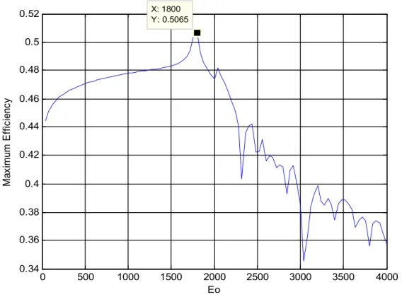
The band-band generation coefficient given by the parameter Y is due to the absorption of photons. The solar cell energy conversion is also dependent to this parameter. The simplest model of the band-trap impact ionization phenomenon doesn’t take into account this parameter. Taking it into account in this study permits us to evaluate the effectiveness real approximate value of the maximum efficiency for solar cell band-trap impact ionization. The diagram of fig.6 shows that the maximum efficiency increases with the increase of the parameter Y. This result permits us to validate the proposed model of the maximum efficiency evaluation. As one could see in the diagram of fig.7, the maximum efficiency of solar cell band-trap impact ionization can reach the value of 50.65 % for Y= 4×1022 Cm-3.S-1.

0 500 1000 1500 2000 2500 3000 3500 4000 0.3 0.32 0.34 0.36 0.38 0.4 0.42 0.44 X: 1800 Y: 0.4305 Eo M ax im um E ff ic ien cy

0 1000 2000 3000 4000 ₀ 0.1 0.2 0.3 0.4 0.5 0.3 0.32 0.34 0.36 0.38 0.4 0.42 0.44 t X: 1800 Y: 0.225 Z: 0.4305 Eo M a x im u m E ff ic ie n c y

Fig.5. Diagram plotting maximum efficiency against Eo and t

0 0.5 1 1.5 2 2.5 3 3.5 4 x 1022 0.2 0.25 0.3 0.35 0.4 0.45 0.5 0.55 Y M ax im um E ff ic ie nc y

Fig.6. Maximum efficiency against Y for 0 ≤ Y ≤ 4×1022 Cm-3.S-1 and E0 = 1800 V/Cm

0 500 1000 1500 2000 2500 3000 3500 4000 0.34 0.36 0.38 0.4 0.42 0.44 0.46 0.48 0.5 0.52 Eo M a x im u m E ff ic ie n c y X: 1800 Y: 0.5065

Fig.7. Maximum efficiency for 0 ≤ E0 ≤ 4000 V/Cm and Y = 4×1022 Cm-3.S-1 Table 2 presents the peak of the maximum efficiency for different values of Y. The time parameter has an effect on increasing of the maximum efficiency because the number of free charge carriers increase with time. The diagram of fig.8 shows a fast increase of the maximum efficiency for t ≤ 1000 s. For t ˃ 1000 s, the maximum efficiency increases slowly and tends verse a constant value, this means that there could has a upper limit of the photovoltaic solar cell’s maximum efficiency that could not vary with time during his working.

Table 2. Peak of the maximum efficiency configuration

Eo (V/Cm) Y (Cm-3.S-1) Time (S) Maximum efficiency η (%) 1800 4×1016 0.225 43.05

1800 4×1018 0.225 43.19 1800 4×1020 0.225 45.9 1800 4×1022 0.225 50.65

0 1000 2000 3000 4000 5000 6000 7000 8000 9000 10000 0.2 0.25 0.3 0.35 0.4 0.45 0.5 0.55 t(s) Ma x imu m e ff ic ie n c y (% )

Fig.8. Diagram plotting Maximum efficiency against t for Y = 4×1016 Cm-3.S-1 and E0 = 1800 V/Cm

3. CONCLUSION

This work consisted to propose a new model of photovoltaic solar cell working in dynamical regime. Silicon solar cell band-trap impact ionization has been chosen in this effect. The results showed that electrons and holes densities from which depends the total charge current density have a solitary wave behavior. The maximum efficiency of the new solar cell has been evaluated. For a determinate range of the applied electric field Eo and for different values of the photo-generation coefficient, the peak of the maximum efficiency has been obtained for Eo=1800 V/cm. The impact of the photo-generation coefficient Y on the efficiency of the solar cell has been studied. For strong electric field, there are currents instabilities in the solar cell which reduce his efficiency. The obtained results prove that the band-trap impact ionization phenomenon can improve the efficiency of the solar cell.The obtained results could also permit to avoid the undesirable range of the external applied electric field on solar cell band-trap

impact ionization. The prospect of this work is to reflect on how to generate the external electric field in order to minimize the cost of the solar energy.

4. REFERENCES

[1] Würfel P, Physics of solar cell from principles to new concepts, WILEY-VCH publishers, Weinheim, 2005.

[2] Green M.A., Third Generation Photovoltaics, Springer Verlag, 2003. [3] M. A., Proceedings 16th E.C. PV solar Energy Conf, 2000, pp. 51.

[4] Yamaguchi M et al., Proc. 19. EU Photovoltaic Solar Energy Conference, Paris, 2004. [5] Swanson R.M., Proc. 8. E.C., Photovoltaic Solar Energy Conference, Florence 1998. [6] Schöll E, Nonequilibrium Phase Transition in semiconductor Self-organisation Induced by Generation and Recombination Processes, Springer Verlag, Berlin, 1987.

[7] Aoki K., amamoto KY, Non-linear response and chaos in semiconductor induced by impact ionization, Appl. Phys. A 48, 1989, pp. 111-125.

[8] Schöll E, Nonlinear Spatio-Temporal Dynamics in Semiconductors, Brazilian Journal of Physics, 29(4), 1999.

[9] Werner J., Brendel R., Queisser H.J, First World Conf. on Photovoltaic Energy Conversion, Hawaii, 1994.

[10] Stephen J. Fonash, Solar cell device physics, second edition, Elsevier Inc, 2010.

[11] Mibaile J et al, Chaos in semiconductor band-trap impact ionization, Current Applied Physics, 13, 2013, pp. 1209-1212.

[12] Schöll E, Modeling nonlinear and chaotic dynamics in semiconductor device structure, VLSI, Design 6, 1998, pp. 321-329.

[13] Shaw M.P., Mitin V.V., Schöll E and Grubin H.L, The Physics of instabilities in Solid State Electron Devices, Plenum Press, New York, 1992.

[14] Kerner B.S. and Osipov V.V, Autosolitons, Kluwer Academic Publishers, Dordrecht, 1994. [15] Niedermostheide F.J, Nonlinear Dynamics and Pattern Formation in semiconductors and Devices, Springer, 1995.

impact ionization, Appl. Phys. A 48, 1989, pp. 111-125.

[17] Abé Y, Nonlinear and chaotic transport phenomena in semiconductors, Appl. Phys, A 48, 1989, 93-191.

[18] Kazunori A, Rule dynamics of turbulence in semiconductors caused by impact ionization Avalanche, Int. J. Bifurcation and Chaos 7, 1997, pp. 1059-1064.

[19] Mayer K.M., Gross R., Parisi J., Peinke J., Huebener R.P., Solid State Commun, 63, 55, 1987.

[20] Mayer K.M., Parisi J., Huebener R.P., Z. Phys. B-Condensed Matter 71, 171, 1988. [21] Mibaile J et al, Exact solutions of a semiconductor non linear reaction diffusion equation through factorization method, Applied Mathematics and Computation, 219, 2012, pp. 2917-2922.

[22] Rosu H.C. and Cornejo-Pérez O, Super symmetric pairing of kinks for polynomial nonlinearities, Phys. Rev. E 71, 2005, 046600-046607.

[23] Fahmy E.S, Exact solutions for some Reaction-Diffusion Systems with Nonlinear Reaction Polynomials Terms, Applied Mathematical Sciences, 3, 2009, pp. 533-540.

[24] Zhen Y.G et al, Dielectric response and its light-induced change in undoped a-si:H films below 13 MHz, Phys. Rev. B 57,1998, pp. 2387-2392.

How to cite this article:

Zieba Falama R, Justin M, Djongyang N and Yamigno Doka S. A Novel Technique for improving the efficiency of a photovoltaic silicon solar cell based on the band-trap impact ionization phenomenon. J. Fundam. Appl. Sci., 2015, 7(3), 375-393.