CIRPÉE
Centre interuniversitaire sur le risque, les politiques économiques et l’emploi
Cahier de recherche/Working Paper 06-11
Chronic and Transient Poverty: Measurement and Estimation, with
Evidence from China
Jean-Yves Duclos Abdelkrim Araar John Giles
Avril/April 2006
_______________________
Duclos: Département d’économique and CIRPÉE, Pavillon DeSève, Université Laval, Québec, Canada G1K 7P4; phone: 1-418-656-7096; fax: 1-418-656-7798
Araar: CIRPÉE, Pavillon DeSève, Université Laval, Québec, Canada G1K 7P4; phone: 418-656-7507; fax: 1-418-656-7798
Giles: Department of Economics, Michigan State University, 110 Marshall-Adams Hall, East Lansing, MI 448824; phone: 1-517-355-7755
Abstract: The paper contributes to the measurement of poverty and vulnerability in
three ways. First, we propose a new approach to separating poverty into chronic and transient components. Second, we provide corrections for the statistical biases introduced when using a small number of periods to estimate the importance of vulnerability and transient poverty. Third, we apply these tools to the measurement of chronic and transient poverty in China using a rich panel data set that extends over approximately 17 years. We find that alternative measurement techniques yield significantly different estimates of the relative importance of chronic and transient poverty, and that precision of estimates is enhanced with simple statistical corrections.
Keywords: Poverty dynamics; Transient poverty; Chronic poverty; Permanent
poverty; China
1 Introduction
Most poverty measurement takes place in an hypothesized world of certainty. Poverty measures, and the impact of policies on such measures, are indeed usually estimated after all uncertainty surrounding well-being is assumed to have been re-solved.
In some limited instances, this certainty assumption might not seem too strong. It could be argued, for instance, that analysts should be able to infer the ex post impact of some economic policy by comparing measures of well-being before and after introduction of the policy. Policy design, however, rarely takes place with the benefit of hindsight, and the distributive impact of policy can vary widely within classes of agents that are observationally homogeneous ex ante. Some policies also generate a greater average level of well-being but at the cost of greater social and individual risk. In such contexts, ex post policy analysis would seem to be at best incomplete.
This mean/risk tradeoff should be of concern when analyzing the impact of policy, but it is also more generally important when comparing welfare across natural, social and economic environments of varying degrees of risk and ”vul-nerability”1. The term ”vulnerability” has been used with increased frequency
recently, in particular since it was highlighted in the 2001 World Development Report (World Bank, 2001). A large number of definitions of the term exist. In our present context, we can understand it as the impact of risk on the ”threat of poverty, measured ex-ante, before the veil of uncertainty has been lifted” (Calvo and Dercon, 2005, p.2). As Ligon and Schechter (2003) emphasize, ”a household with very low expected consumption expenditures but with no chance of starv-ing may well be poor, but it still might not wish to trade places with a household having a higher expected consumption but greater consumption risk” (p. C95). This paper proposes a new approach to separating total poverty into chronic and transient components, and offers useful and intuitive measures for understanding this mean/risk tradeoff.
This important distinction between low expected well-being and vulnerability is also nicely illustrated by Hulme and McKay (2005):
”Historically, the idea that some people are trapped in poverty while
1Probably the most important source of risk in developing countries is that faced by rural
farming households and linked to uncertain climatic conditions. Other high-risk factors stem from probabilities of illness, unemployment, social exclusion, changes in wages and in prices, removal of family and social protection, and disturbances in productive and exchange environments.
others have spells in poverty was a central element of analysis. For ex-ample, officials and social commentators in eighteenth century France distinguished between the pauvre and the indigent. The former ex-perienced seasonal poverty when crops failed or demand for casual agricultural labour was low. The latter were permanently poor be-cause of ill health (physical and mental), accident, age, alcoholism or other forms of ‘vice’. The central aim of policy was to support the
pauvre in ways that would stop them from becoming indigent.” (p.3)
Thus, not only is ”chronic poverty” different from ”temporary” or ”transient” poverty, but the difference between the two is likely to call for distinct policy attitudes and responses, as stressed for instance in a report of the Chronic Poverty Research Centre (2004)2and as is nicely stated by Jalan and Ravallion (1998):
Increasing the human and physical assets of poor people, or the re-turns to those assets, are thought to be more appropriate to allevi-ate chronic poverty. Insurance and income-stabilization schemes are seen to be more important policy instruments when poverty is tran-sient (Lipton and Ravallion, 1995). Knowing how much the currently observed level of poverty is transient may thus inform policy choices. (p.339)
The current paper also suggests statistical strategies to improve estimators of the relative importance of risk in total ill-fare. With the increased availability of longitudinal data sets, it is now well known3that there is significant movement in
and out of poverty as well as within poverty itself. It is also widely recognized that these findings are very sensitive to the presence of measurement errors — see for instance Rendtel et al. (1998) and Breen and Moisio (2004). An anal-ogous concern arises when only a relatively small number of time observations is available for each individual over time and when the estimators of interest are non-linear across time periods. Other than the present study, most of the literature on the measurement of poverty and vulnerability has ignored biases introduced
2See also the special issue on chronic poverty published in World Development, volume 31,
issue 3, pages 399–665, March 2003.
3See among many others Bane and Ellwood (1986), Gaiha (1988), Gaiha (1989), Jarvis and
Jenkins (1997), Baulch and Hoddinnott (2000), Atkinson et al. (2002), Chaudhuri et al. (2002), Ligon and Schechter (2003), Cruces and Wodon (2003), Bourguignon et al. (2004), Christiaensen and Subbarao (2004), and Kamanou and Morduch (2004).
by a small number of time observations. Unlike corrections for measurement er-rors, which are typically difficult to provide, we demonstrate that corrections for small-number-of-time-periods biases are relatively straightforward to design and to apply.
Our paper thus contributes to the measurement of poverty and vulnerability in three ways. First (Section 2), we follow the recent literature and investigate how we may split the measurement of total poverty into chronic and transient compo-nents, the latter component being generated by the presence of risk. We build on the influential work of Ravallion (1988) and Jalan and Ravallion (1998) and show how money-metric measures of low average well-being (chronic poverty) and risk (transient poverty) can jointly account for total deprivation (total poverty) in a so-ciety.
Second (Section 3), we provide methods for correcting statistical biases in the estimation of chronic and transient poverty. This is important since the number of periods over which well-being is observed is usually relatively small, and since this can distort one’s understanding of the importance of risk in accounting for total ill-fare. Note that these corrections are derived explicitly in this paper for only two alternative measurement systems — Jalan and Ravallion’s and a money-metric one that we develop. The paper’s methodology, however, can be extended to other indices, including those discussed in Chaudhuri et al. (2002), Ligon and Schechter (2003), Suryahadi and Sumarto (2003), Christiaensen and Subbarao (2004), Kamanou and Morduch (2004), and Kurosaki (2005).
Third (Section 4), we apply these tools to the measurement of chronic and tran-sient poverty in China using a rich panel data set that extends over approximately 17 years. We find inter alia that alternative measurement techniques can give very different views on the relative importance of chronic and transient poverty, and that statistical bias corrections can significantly enhance the precision of such poverty estimates. Section 5 concludes the paper.
2 Measuring chronic and transient poverty
2.1 Measuring poverty
Consider a vector y = (y1, y2, ..., yn) of living standards yi(incomes4, for short) for n individuals, where yi = (yi1, yi2, ..., yit) is itself a vector of individual i’s incomes across t periods. For expositional simplicity, we assume that each income
yij has been normalized initially by the poverty line in period j. An individual i with yij = 1$ is thus exactly at the poverty line at time j. A useful tool in this paper will be that of (normalized) poverty gaps, defined for an income yij as
gij = (1 − yij)+, (1) where f+ = max(f, 0). The vectors g = (g1, g2, ..., gn) and gi = (gi1, gi2, ..., git) are then the corresponding vectors of poverty gaps. Many of the common poverty measures can be expressed in terms of such poverty gaps5. An important subset of
these measures is the well-known class of the FGT (Foster, Greer and Thorbecke, 1984) additively decomposable indices. Over the n individuals and the t periods, and thus over the vector g, the FGT indices are defined as
Pα(g) = (nt)−1 n X i=1 t X j=1 gijα. (2)
When α = 0, (2) gives the proportion of the t time periods over which the n indi-viduals have been poor; when α = 1, (2) gives the average poverty gap over the t time periods and the n individuals; and for α > 1, (2) yields poverty indices that are sensitive to the distribution of poverty gaps and give greater ethical weights to greater poverty gaps.
Pα(gi) for individual i s analogously defined as
Pα(gi) = t−1 t X j=1 gα ij. (3)
Note that α ≥ 0 may be considered as a measure of ”poverty aversion”, namely, a measure of aversion to inequality and variability in the poverty gaps: a larger α
4Note that we do not discuss here the more general problem of the relative advantages and
disadvantages of using monetary vs non-monetary indicators for assessing chronic and transient poverty. See e.g. Hulme and McKay (2005) for a discussion of this issue.
5Note that focussing on poverty gap measures is not needed for the analysis, although it
gives a relatively greater weight to a loss of income when income is already low than when it is large. It is also well-known that the headcount P0 can increase
following a mean-preserving equalizing transfer of income. The same is true for a mean-preserving decrease in the variability of income over time: this can increase
P0(g). For these reasons, we exclude the headcount from the analysis (for now)
and also assume that α ≥ 1.
As noted above, P1(g) yields the average poverty gap, whose sensitivity to
changes in incomes is the same regardless of the income of the poor (so long as the poor remain poor). When α > 1, a marginal equalizing transfer of income from a poor person to anyone who is poorer decreases Pα(g), thus making these indices ”distribution” and ”variability” sensitive.
2.2 Jalan and Ravallion’s chronic and transient poverty
Jalan and Ravallion (1998) (JR, for short) use Pα(g) to propose intuitive measures of ”chronic” and ”transient” poverty. To see how, note that byi = t−1Pt
j=1yijis an estimate of i’s ”permanent income” over the t periods. JR argue that an estimate of the ”chronic” poverty of an individual i can be obtained by replacing his income
yij for all periods j by estimated permanent income. t−1 Pt j=1 ³ 1 − byi ´α + is then
i’s chronic poverty. Summing across all individuals, aggregate chronic poverty
would then be equal to6
P∗ α(y) = n−1 n X i=1 ³ 1 − byi ´α +. (4)
The difference between total poverty, Pα(g), and chronic poverty, Pα∗(y), can then be interpreted as a measure of transient poverty, PT
α(y), which is thus given by:
PαT(y) = Pα(g) − Pα∗(y). (5) Although intuitive and simple, the above formulation has a few disadvantages:
6Note that JR’s definition (and ours) differs conceptually from that in Chronic Poverty
Re-search Centre (2004), where chronic poverty is defined as ”poverty experienced by individuals and households for extended periods of time or throughout their entire lives” (p. 131) and where transitory poverty is defined as ”poverty experienced as the result of a temporary fall in income or expenditure although over a longer period the household resources are on average sufficient to keep the household above the poverty line” (p. 132).
• It is well-known that an increase in α gives greater relative weight to the
ill-fare of the poorest. An increase in α thus makes the poverty index more representative of the ill-fare of the poorest among the poor, and should thus increase measured poverty. But it is easily checked that Pα(g) decreases with α. (This feature often causes confusion in the applied poverty liter-ature.) In the current chronic-transient setting, an increase in α will also decrease all of Pα(g), Pα∗(y), and PαT(y), leading to the additional awk-ward result that an increase in poverty aversion decreases the measure of both transient and chronic poverty.
• The Pα(g) (and Pα∗(y) and PαT(y)) indices have no obvious cardinal
inter-pretation when α differs from 0 or 1. The basic reason is that their mea-surement units are in dollars to the power α. This is in contrast to much of the literature on inequality and social welfare, in which the indices are either unit free or are in dollars. This property of the JR indices also makes it difficult to use them in conjunction with the money-metric indicators that are common in efficiency and cost-benefit analysis.
• A more minor point concerns the construction of the P∗
α(y) chronic poverty index. As shown in (4), this is assessed using average income over t time periods. Hence, someone in severe poverty over t − 1 periods may still be deemed to have zero chronic poverty if his income during the tthperiod is large enough to make average income over the t periods be above 1. One alternative is to use the average of incomes censored at the poverty line — an idea we explore below in the illustrative section. Another alternative is to consider chronic poverty to be a measure of ”average” poverty — measured as an average of the poverty status experienced over the t periods. This is
inter alia what we propose to do in the following sections.
2.3 EDE poverty gaps
A simple monotonic transformation of Pα leads to a useful money-metric sure of poverty. In the manner of Kolm (1969) and Atkinson (1970) for the mea-surement of social welfare and inequality, let Γα(g) be the ”equally-distributed equivalent” (EDE) poverty gap, viz, that poverty gap which, if assigned equally to all individuals and in all periods, would produce the same poverty measure as that generated by the distribution g of poverty gaps. Using (2), Γα(g) is given
implicitly as
Γα(g)α ≡ Pα(g), (6) and thus we have that
Γα(g) = Pα(g)
1
α. (7)
Note that Γ1(g) is again the average poverty gap. As mentioned above, using
Γ1(g) as a measure of poverty fails to take into account the inequality in poverty
statuses. Inequality in poverty presumably raises the social cost of poverty above the level of what poverty would be if it were equally spread. This suggests that an inequality-corrected measure of poverty should in general be no less than Γ1(g)
in order for poverty to be sensitive to the presence of inequality among the poor. Such a property holds for Γα(g) whenever α is greater than or equal to 1.
Whenever all have the same poverty gap, we have that Γα(g) = Γ1(g). A
mean-preserving increase in the income spread between two individuals (with at least one of them being poor) strictly increases Γα(g) whenever α is strictly greater than 1. Thus, for a given α, the more important the difference between Γα(g) and Γ1(g), the more unequal the distribution of poverty gaps. An obvious
measure of the cost of inequality in the distribution of poverty gaps is then given by:
Cα(g) = Γα(g) − Γ1(g). (8)
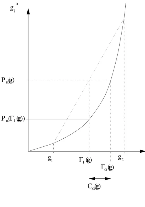
Note that Cα(g) is given in per capita money-metric terms, which makes it di-rectly comparable to Γ1(g) and other money-metric indicators. Cα(g) is the cost in average poverty gap that a Social Decision Maker (SDM) would be willing to pay to remove all inequality in the distribution of poverty gaps, without a change in total poverty — recall Atkinson (1970) for a similar interpretation in terms of social welfare. Cα(g) is always non-negative. Rewriting (8), total poverty can be expressed as
Γα(g) = Γ1(g) + Cα(g). (9) This is illustrated in Figure 1. Figure 1 shows a distribution of 2 poverty gaps,
g1 and g2 (measured along the horizontal axis), the poverty index Pα(g) for that distribution, the average poverty gap Γ1(g), and the EDE poverty gap Γα(g). Note that Γ1(g) is the average of g1 and g2, and that Γα(g)α = Pα(g) is the average of
gα
1 and g2α. The cost of inequality in poverty gaps is then the horizontal distance
2.4 Transient and chronic poverty with the EDE poverty gap
approach
Transient poverty generates variability and thus inequality in the poverty status of individuals. It is thus natural to use the framework described above to capture its importance. Let γα(gi) be the EDE poverty gap for individual i, namely,
γα(gi) = Ã t−1X j=1 gα ij !1/α . (10)
Using the cost-of-inequality approach introduced above, a natural measure of the cost of the transient component of i’s poverty status is then given by
θα(gi) = γα(gi) − γ1(gi), (11) which is again non-negative for any α ≥ 1. The EDE gap γα(gi) can be in-terpreted as the variability-adjusted poverty status of individual i. γ1(gi) is i’s average poverty gap. In a context of risk aversion in which an individual i would augment ex ante his expected poverty gap by a risk premium, this risk premium would be given by θα(gi), and his variability-adjusted poverty status would thus be given by γ1(gi) + θα(gi). Analogously to the SDM mentioned above, individ-ual i would be willing to pay up to θα(gi) in units of his average poverty gap to remove variability in his poverty gap status.
A natural next step is to aggregate the transiency cost θα(gi) across the n individuals in order to obtain the aggregate magnitude of transiency, denoted as ΓT
α(g). This is given simply by:
ΓTα(g) = n−1 n X i=1 θα(gi). (12) ΓT
α(g) can also be interpreted as the cost of inequality within individuals.
Let us now focus on the distribution of the individual EDE poverty gaps
γα(gi). This distribution is the distribution of individual ill-fare in the pres-ence of both individual chronic and transient poverty. Denote this distribution by γα = (γα(g1), ..., γα(gn)). Aggregate poverty with γα is then given by
Γα(γα) = Ã n−1 n X i=1 γα(gi)α !1/α . (13)
The cost of inequality in the EDE poverty gaps γαthen equals
Cα(γα) = Γα(γα) − Γ1(γα). (14)
Cα(γα) can thus be interpreted as the cost of inequality between individuals. This leads to the following result:
Theorem 1 Total poverty is given by the sum of the average poverty gap in the
population (Γ1(g)), the cost of inequality in individual EDE poverty gaps (Cα(γα)),
and the cost of transient poverty (ΓT
α(g)):
Γα(g) = Γ1(g) + Cα(γα) + ΓTα(g). (15) See the Appendix.
Given the result of Theorem 1, it is natural to define chronic poverty as the dif-ference between total and transient poverty, and chronic poverty is hence denoted as
Γ∗(g) = Γ
1(g) + Cα(γα). (16) Chronic poverty is then the average poverty gap plus the cost of inequality in EDE poverty gaps across individuals. Transient poverty is the cost of the variability of poverty gaps across time.
Corollary 2 Total poverty is the sum of chronic and transient poverty:
Γα(g) = Γ∗(g) + ΓTα(g). (17) Note that the total cost of inequality in poverty gaps is the sum of the cost of inequality between individuals and that of inequality within individuals:
Cα(g) | {z } total inequality = C| {z }α(γα) between individuals + ΓT α(g) | {z } within individuals . (18)
All three expressions in (18) are increasing in α. They are also increasing in the inequality of poverty gaps: a mean-preserving inequality-increasing change in the EDE poverty gaps will increase Cα(γα), and a mean-preserving variability-increasing change in the temporal distribution of poverty gaps will increase ΓT
α(g). Both of these changes will therefore increase Cα(g) and Γα(g). All three expres-sions in (18) also have a money-metric interpretation: Cα(g) is the cost in average poverty gap units that a SDM would be willing to incur to remove all variability in poverty status, Cα(γα) is the cost that a SDM would be willing to incur to remove between-individual inequality in welfare status, and ΓT
α(g) is the cost that individ-uals would collectively be willing to incur to remove within-individual variability in poverty status.
2.5 Graphical interpretation
Figures 1 and 2 help to clarify the relationship between the two measures of chronic and transient poverty. The fundamental distinction between the JR and the EDE approaches comes down to whether we measure poverty on the ver-tical or on the horizontal axis of Figure 1 — if we think of g1 and g2 as the
poverty gaps of one individual across two periods. The JR approach roughly7
expresses chronic poverty as Pα(Γ1(g)) and transient poverty as the difference
Pα(g) − Pα(Γ1(g)), both of which can be seen on the vertical axis of Figure 1.
The EDE approach defines chronic poverty as Γ1(g) and transient poverty as the
difference Γα(g) − Γ1(g), both of which can be measured on the horizontal axis
of Figure 1.
Figure 2 extends Figure 1 to the case of two individuals and therefore also allows for a depiction of the importance of between-individual inequality. Four poverty gaps are shown, two for individuals 1 (g11and g12) and two for individuals
2 (g21and g22). Their average poverty gaps are shown by γ1(g1) and γ1(g2). Their
EDE poverty gaps are given by γα(g1) and γα(g2). The costs of transiency in their
poverty status are thus given by the distance γα(gi) − γ1(gi) for each of i = 1, 2. The average of these costs across the two individuals gives ΓT(g) (recall equation (12)), and ΓT(g) is also the difference on Figure 2 between Γ
1(γα) and the overall poverty gap Γ1(g). ΓT(g) is thus the cost of within-individual inequality. The cost
of between-individual inequality is given by the difference Γα(g) − Γ1(γα). The total cost of inequality is the sum of between- and within-individual inequality and equals Γα(g) − Γ1(g) on Figure 2. Adding that total cost of inequality to the
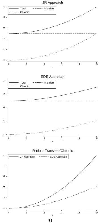
overall average poverty gap Γ1(g) gives the overall EDE poverty gap, Γα(g). The JR and EDE approaches thus measure chronic and transient poverty differ-ently. To illustrate further this distinction, let the poverty gap for an hypothetical household i be defined for two periods 1 and 2 by
gi1= 0.5 − e, (19)
gi2= 0.5 + e, (20)
where e ∈ [0, 0.5] captures the variability in poverty status across time. For α = 2,
7Only ”roughly”, since the JR approach uses average income over time — and not the average
it is not difficult to check that
JR total poverty = 0.25 + e2
JR chronic poverty = 0.25 JR transient poverty = e2
EDE total poverty =√0.25 + e2 (21)
EDE chronic poverty = 0.5
EDE transient poverty =√0.25 + e2− 0.5. (22)
Figure 3 shows these poverty estimates according to the JR and EDE ap-proaches, both in absolute value and as a proportion of chronic and total poverty, and also as a function of e. For both approaches, chronic poverty is invariant with
e. Although the impact of e on transient and total poverty is qualitatively similar
in this example for both the JR and the EDE approaches, numerically the esti-mates are quite different — as we will also find in the illustrative Section 4 below. Since the EDE components are expressed in money-metric terms, one can check that EDE total and transient poverty are of the same order of magnitude as e, but that JR total and transient poverty are of the order of eα. Take the case of g
11 = 0
and g12= 1. On the one hand, the JR approach gives equal value to chronic (0.25)
and to transient poverty (0.25), leading to an estimate of total poverty (0.5) that is twice as large as that of chronic poverty. Although it would seem impossible to draw a social consensus on a precise normative valuation of the different com-ponents of poverty, it would appear implausible that a sole movement of 0.5 on either side of a chronic gap of 0.5 be given the same poverty importance as that chronic gap itself. On the other hand, the EDE approach yields an estimate of total poverty (0.71) that is about 50% larger than chronic poverty (0.5), thus implying that the social cost of a movement of 0.5 on either side of a chronic gap of 0.5 is lower than the cost of the chronic gap itself.
3 Statistical procedures
Sections 2.2 and 2.4 provide two alternative approaches to distinguishing between total and transient poverty. JR’s approach first defines an individual’s chronic poverty as poverty when he is assumed to earn his permanent income, and then defines transient poverty as the difference between total and chronic poverty. The approach of Section 2.4 first defines an individual’s transient poverty as the
dif-ference between his EDE and his average poverty gap, and then measures chronic poverty as the difference between total and aggregate transient poverty.
Both approaches can in practice be easily implemented using panel data. Such panel data will, however, typically involve a relatively modest number of time periods, t. As we will see, this in turn can create substantial systematic differences between sample estimates and the value of the true (unobserved) poverty indices. With JR’s approach, these biases will directly affect the estimation of chronic poverty. With the EDE approach of Section 2.4, these statistical biases will have a direct effect on the estimation of transient poverty. Transient poverty (for JR) and chronic poverty (for the EDE approach) will also be biased since they are obtained as differences between biased estimators. We thus introduce procedures that correct, at least partially, for these biases.
3.1 Analytical bias corrections
For each individual i, i = 1, ..., n, t income values are assumed to be drawn randomly from a distribution function Fi(y). For expositional simplicity, income is normalized by the fixed and known poverty line and its distribution Fi(y) is also assumed constant across periods. This generates a sample of nt incomes denoted as {yi1, ..., yit}ni=1.
3.1.1 Jalan and Ravallion’s chronic-transient poverty
Let yithen be the expected income of individual i — his permanent income. This is defined as yi = R ydFi(y). An individual i’s true (as opposed to estimated) chronic poverty is then given by
P∗
α,i = (1 − yi)α+. (23)
A natural estimator of yi with panel data is byi = t−1Pt
j=1yij, where yij is the observed sample income of individual i at time j. An obvious estimator for P∗
α,i is simply
³ 1 − byi
´α
+. This, however, is biased upwards for finite values of t since
we can show that (see Appendix)
E ·³ 1 − byi ´α + ¸ = P∗ α,i+ α(α − 1) 2t (1 − yi) α−2 + var(yij) + O(t−2) (24) ≥ P∗ α,i, (25)
where var(yij) = R
(y − yi)2dFi(y). Hence, an estimator that includes a second-order correction for the bias of
³ 1 − byi
´α
+is given by cP
∗
α,iand is defined as c P∗ α,i = ³ 1 − byi ´α ++ α(1 − α) 2t (1 − yi) α−2 + var(yij). (26) The Appendix also shows how to incorporate higher-order bias corrections, al-though these did not prove to be very useful in our Monte Carlo simulations. Note that all of the elements in (26) can be estimated consistently, inter alia by substi-tuting byifor yi and (t − 1)−1Pt
j=1 ³
yij − byi
´2
for var(yij). (26) thus provides an easily implementable second-order correction for JR’s index of chronic poverty. 3.1.2 EDE chronic-transient poverty
We now turn to a second-order bias correction for the estimation of this pa-per’s proposed measure of transient poverty. Let γα,i be the true (as opposed to the estimated) EDE poverty gap of individual i. This is defined as γα,i = ¡R
(1 − y)α+dFi(y) ¢1/α
. A natural estimator of γα,i is given by γα(gi) (recall equation (10)). But this estimator is again biased for small values of t because
γα(gi) is non linear in gij. Defining Pα,i = R
(1 − y)α+dFi(y), this bias is shown by the fact that (see the Appendix for a fuller demonstration)
E [γα(gi)] = E h γα,i+ α−1γ(1−α) α,i £ Pα(gi) − Pα,i ¤ −0.5α−2(α − 1)γ(1−2α)α,i £Pα(gi) − Pα,i ¤2i + O(t−2). (27) Since E£Pα(gi) − Pα,i ¤ = 0 and Eh¡Pα(gi) − Pα,i ¢2i = t−1var(gα ij), we have (to leading order) that
E [γα(gi)] ∼= γα,i− 0.5α−2(α − 1)γ
(1−2α)
α,i t−1var(gijα) (28)
≤ γα,i. (29)
This shows that γα(gi) is biased downwards. A second-order correction for γα,i is thus given by
b
Again, all of the elements in (30) can be estimated consistently. γ(1−2α)α,i
can be estimated as Pα(gi)(1−2α)/α and var(gijα) can be estimated as (t − 1)−1Pt j=1 ¡ gα ij − Pα(gi) ¢2 .
3.2 Bootstrap bias corrections
An alternative approach to correcting for the biases found in (25) and (29) is by estimating the biases that arise in numerical simulations of the longitudinal butions of incomes. One way to proceed is by bootstrapping the empirical distri-bution of each subsample of t periods’ incomes. This can be done as follows:
1. For each individual i, we wish to compute an estimator η³ iof chronic poverty 1 − byi
´α
+or of transient poverty γα(gi).
2. For each individual i, we first compute a ”plug-in” estimator using i’s origi-nal sub-sample of t incomes, {yi1, ..., yit}; this is either
³ 1 − byi
´α
+or γα(gi).
3. For each individual i and for each of k = 1, ..., K, we generate a sam-ple of t incomes drawn randomly (and with replacement) from the original sub-sample of t incomes for individual i, {yi1, ..., yit}. We compute a new estimator ηk
i for each such simulated sample k. We should choose K to be as large as is numerically sufficient and computationally reasonable. 4. ηB
i is given by the mean of these K estimators ηik, that is, we have ηBi =
K−1PK
k=1ηik. The bootstrap estimate of the bias is then given by the dif-ference between ηB
i and the plug-in estimator. Each of
³ 1 − byi
´α
+and γα(gi) can then be corrected by the bootstrap-estimated
bias ηB i − ³ 1 − byi ´α + or η B
i − γα(gi). The corrected estimator of JR’s index of chronic poverty is given by
f P∗ α,i = 2 ³ 1 − byi ´α +− η B i (31)
and a bootstrap-corrected estimator of Section 2.4’s index of transient poverty is given by
e
3.3 Bias corrections: Monte Carlo evidence
To explore the performance of the above bias-correction methods, we use Monte Carlo simulations to estimate the statistics of interest (total, chronic, and transient poverty) with and without bias corrections. To do this:
1. We assume a log-normal longitudinal distribution of incomes with mean and standard deviation both set to 1 (recall that incomes are normalized by the poverty line). We compute the statistics of interest for that distribution. 2. We choose a number t of longitudinal income observations to be drawn
randomly and independently from that population.
3. For each of h = 1, ..., H, we draw a sample of t such observations and estimate the statistics of interest, with or without bias corrections.
4. We compute the average of the H statistics estimated in the previous step, and compare that average to the true population statistics calculated in step 1.
Note again that step 2 above can be done with or without bias corrections. Recall that biases arise because of the finite number of periods, not because of a finite number of households.
The Monte Carlo evidence is shown on Figure 4 for both JR’s chronic poverty and EDE transient poverty, for α = 2 and α = 3, and for a poverty line z set to 1.5 (H was set to 10000; results for z=1 are very similar). The second-order analytical and bootstrap bias corrections work relatively well in all cases, generally reducing by more (and often by much more) than 50% the biases of the naive estimators of chronic and transient poverty. This is true even for the smallest possible number
t = 2 of time periods: in all cases (except for JR’s chronic poverty), the biases
are reduced by roughly 50%. The percentage fall in the biases introduced by the corrections increases with t — although the absolute value of the corrections it-self naturally falls with t. The bias corrections are particularly effective for EDE poverty, apparently because the correction uses the variance in a censored vari-able (compare (26) and (30)). Analytical and bootstrap corrections work almost equally well: EDE transient poverty with α = 3 is only slightly better estimated on average with a bootstrap correction, but JR’s chronic poverty with both α = 2 and α = 3 is on average estimated better with an analytical correction.
Note that the top left-hand (northwest) panel on Figure 4 also shows the bias correction for an uncensored version of the estimator of JR’s chronic poverty, i.e.,
for ¡
1 − ˆyi¢α (33)
(compare with (23)). Although the true population value is unchanged compared to (23), the second-order analytical bias correction now removes completely the bias. This suggests that the JR biases that are left after the corrections shown on Figure 4 are mostly due to the censored form of the estimator of chronic poverty.
4 Illustration: An application to China
4.1 Poverty in Rural China
We illustrate the use of the above methodology with panel survey data from rural China. Much research effort has gone into analyses of the causes and conse-quences of increasing income inequality in China, but the study of poverty and poverty dynamics has received much less attention.8 Recent descriptive research
emphasizes the marked decline in incidence of extreme poverty over twenty-five years of economic reform in China, though it is apparent that pockets of poverty remain (Khan, 2005; Ravallion and Chen, 2005). Jalan and Ravallion (2002), for example, noted the presence of geographic poverty traps and suggest that they may be exacerbated by obstacles to mobility of labor and capital.
Jalan and Ravallion (1998) provide the only attempt to distinguish transient from chronic poverty in rural China, but evidence from related research suggests that exits from poverty are not necessarily permanent and that the possibility of falling into poverty continues to influence the consumption decisions rural house-holds. Giles and Yoo (2005) show that precautionary motives lead to lower con-sumption of households exposed to agro-climatic sources of risk, and Park (2005) finds that households in China’s poor areas store inefficiently high levels of grain in response to expected price variability. Benjamin et al. (2005) document trends in poverty and show that poverty rates can vary considerably with changes in the market price of grains or other economic shocks. Indeed, after a decline in poverty with rising agricultural prices through 1995, poverty rates rose again significantly by 1999.
8Reviews of the inequality literature can be found in Benjamin, Brandt and Giles, 2005, and in
4.2 The RCRE Household Surveys
The data come from annual household surveys conducted by the Survey Depart-ment of the Research Center on Rural Economy (RCRE) in Beijing. We use household level surveys from 82 villages in nine provinces (Anhui, Gansu, Guang-dong, Henan, Hunan, Jiangsu, Jilin, Shanxi, and Sichuan) where households were surveyed annually from 1986 through 2002, with gaps in 1992 and 1994 when funding difficulties prevented survey activities.9 In each province, counties in
the upper, middle and lower income terciles were selected, from which a vil-lage was then randomly chosen. Depending on vilvil-lage size, between 40 and 120 households were randomly surveyed in each village. The panel component of the household survey (from panel villages) includes 3983 households per year from 1987 to 2002.
The RCRE household survey collected detailed household-level information on incomes and expenditures, education, labor supply, asset ownership, land hold-ings, savhold-ings, formal and informal access to credit, and remittances.10 In common
with the National Bureau of Statistics (NBS) Rural Household Survey, respondent households keep daily diaries of income and expenditure, and a resident admin-istrator living in the county seat visits with households once a month to collect information from the diaries.
Our measure of consumption includes nondurable goods expenditure plus an imputed flow of services from household durable goods and housing. In order to convert the stock of durables into a flow of consumption services, we assume that current and past investments in housing are “consumed” over a 20-year period and that investments in durable goods are consumed over a period of 7 years. We also annually “inflate” the value of the stock of durables to reflect the increase in durable goods’ prices over the period. Finally, we deflate all income and ex-penditure data to 1990 prices using the NBS rural consumer price index for each province.
There has been some debate over the representativeness of both the RCRE
9These 82 villages are a subsample of the 110 villages originally surveyed in 1986 in which
survey administrators successfully followed a significant share of households through 2002. The complete RCRE survey covers over 22,000 households in 300 villages in 31 provinces and admin-istrative regions. RCRE’s complete national survey is 31 percent of the annual size of the NBS rural household survey. By agreement, we have obtained access to data from nine provinces, or roughly one-third of the RCRE survey.
10One shortcoming of the survey is the lack of individual-level information. However, we know
the number of dependents and individuals working, as well as the gender composition of household members.
and NBS surveys, and concern over differences between trends in poverty and inequality in the NBS and RCRE surveys. These issues are reviewed extensively in Appendix B of Benjamin et al. (2005), but it is worth summarizing some of the findings from the discussion of that paper. First, when comparing cross sec-tions of the NBS and RCRE surveys with overlapping years from cross section surveys not using a diary method, it is apparent that some high and low income households are under-represented.11 Poorer illiterate households are likely to be
under-represented because enumerators find it difficult to implement and moni-tor the diary-based survey, and refusal rates are likely to be high among affluent households who find the diary reporting method a costly use of their time. Sec-ond, much of the difference between levels and trends from the NBS and RCRE surveys can be explained by differences in the valuation of home-produced grain and treatment of taxes and fees.
4.3 JR and EDE poverty gaps
We use per capita household income and weight households by their sam-pling weight times household size. All expenditures have been normalized by a consumption-based poverty line based on a 2100-calorie-diet plus per capita expenditures for durables and housing of individuals close to poverty line — see Ravallion and Chen (2005)12. Variances for the asymptotically
normally-distributed estimators13of chronic and transient poverty are analytically computed
taking full account of the survey design, viz, taking into account sampling stratifi-cation and clustering14.
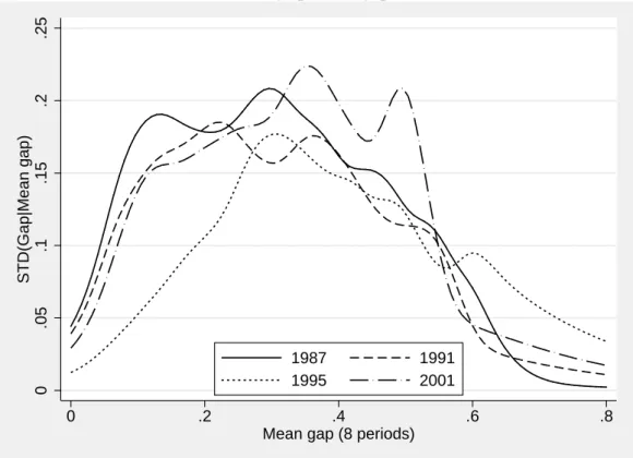
Figure 5 graphs the conditional standard deviation of poverty gaps gt =
11The cross-sections used were the rural samples of the 1993, 1997 and 2000 China Health and
Nutrition Survey (CHNS) and a survey conducted in 2000 by the Center for Chinese Agricultural Policy (CCAP) with Scott Rozelle (UC Davis) and Loren Brandt (University of Toronto).
12This rounds up to a national poverty line of 850 RMB per capita in 2002 that is deflated to
1990 using provincial price deflators.
13The asymptotic results are obtained as n increases to infinity. Since the bias corrections can
be incomplete with a finite number t of time observations, the mean square error and the variance of the estimators can also diverge even as n tends to infinity. Strictly speaking, therefore, the asymptotic analysis is valid only when both n and t tend to infinity. Depending on the order of the imperfection of the bias corrections (see (48) and (54)), the speed with which t needs to increase can, however, be significantly lower than that of n.
14The estimation was done using the freely available DAD program, which can be downloaded
from www.mimap.ecn.ulaval.ca. STATA program files to carry out the estimation are also avail-able upon request.
(g1t, g2t, ..., gnt) at different values of individual average poverty gaps Pα(gi) (these averages are computed at the individual level across 8 time periods of the RCRE surveys separated by a two-year interval between 1987 and 2001) for the poverty gaps prevailing in time period t = 1987, 1991, 1995 and 2001. These conditional standard deviations are estimated non-parametrically using kernel av-eraging of the distance between individual poverty gaps at time period t and the average of these gaps across time for each individual. As can be seen from the Figure, poverty gaps are most variable for those individuals in the middle of the distribution of poverty gaps. Those with an average poverty gap close to 1 are almost always desperately poor, and the variability of their poverty status across time is thus quite low. Those with an average poverty gap close to 0 are almost always very close to or above the poverty line, and the variability of their poverty status across time is thus also very low. No one period appears to dominate clearly the others in terms of poverty variability.
We now carry out a decomposition of total JR poverty using 8 time periods separated by a two-year interval between 1987 and 2001. As shown in Table 1, transient poverty is according to the JR estimates significantly more important than chronic poverty and it represents close to two thirds of total poverty. As expected, the asymptotic and bootstrap bias corrections generate almost identical estimates (these results are rounded to the fourth decimals); with these corrections, transient poverty amounts to about 73% of total poverty. This is in line with the simulation results discussed in Section 3.3. (All of the estimates discussed from now onwards are corrected using second-order analytical bias corrections.)
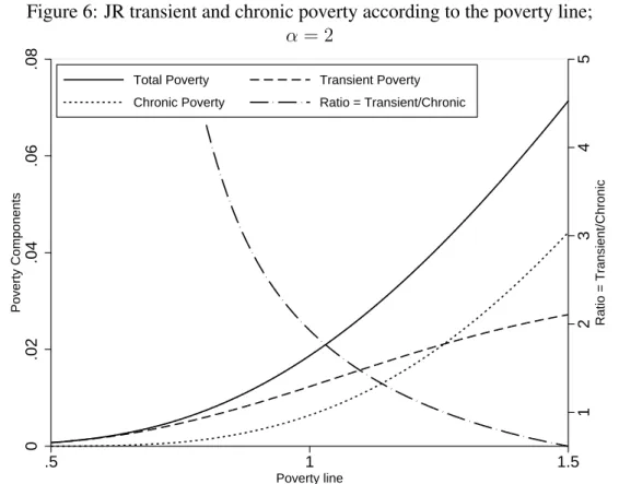
Figures 6 and 7 show the sensitivity of the above results to the choice of the poverty line and of the parameter α. The left vertical axis shows the numerical value of the estimates while the right vertical axis displays the ratio of transient over chronic poverty. For α = 2 in Figure 6, increasing the poverty line from 50% to 150% of the official poverty line naturally increases all of the poverty estimates, but the effect is stronger for chronic poverty. The ratio of transient to chronic poverty is extremely sensitive to the choice of the poverty line, moving from a ratio of 8 to less than 1 when the poverty line varies from 75% to 150% of the official poverty line.
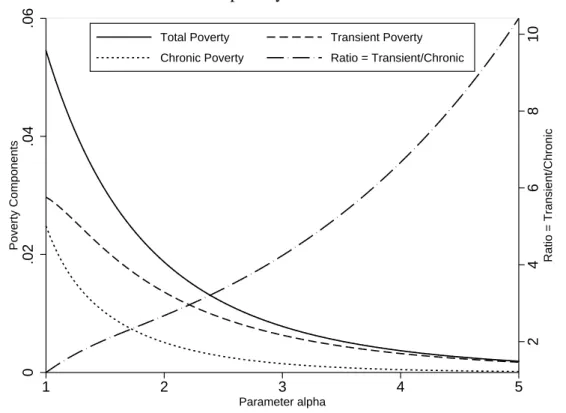
Completely opposite results are obtained in Figure 7 when α increases. As α rises, poverty measurement becomes more and more sensitive to the occurrence of very low incomes, and less to the levels of average incomes. This is evident in Figure 7: for a poverty line set to 1, the ratio of transient to chronic poverty shown on the right vertical axis increases rapidly with α — from 1.2 to more than 10 as α moves from 1 to 5. Note here the graphical verification of the anomaly
mentioned on page 7: all components of the JR decomposition fall numerically with increases in α.
As mentioned above on page 7, the JR approach replaces average uncensored incomes by the average of incomes censored at the poverty line to estimate chronic poverty. The use of average uncensored incomes assumes that households are able to abide by the permanent income hypothesis. Credit constraints, risk aversion and behavioral difficulties to save can, however, render this invalid. Using instead the average of incomes censored at the poverty line would basically assume that individuals are able to smooth their consumption behavior when incomes are no greater than z, but that they are not able to save any of the excess incomes that would bring (e.g., temporarily large or windfall) incomes above the poverty line.
To see how to account for this analytically, let ˙yij = min(yij, z) be income
yij censored at z. We can then re-estimate all of the JR poverty components with ˙yij instead of yij. It can be checked that the estimate of total poverty bPα(g) will remain unchanged, but the estimation of i’s chronic poverty will now use b˙yi = t−1Pt
j=1 ˙yij instead of byi, with corresponding changes to the estimation of aggregate chronic poverty and transient poverty.
To see what this does to the estimates, we carry out the JR decomposition with censored incomes and report the results in Table 2. As mentioned, this does not change total poverty, but it has a considerable impact on its two components. Bias-corrected chronic poverty increases from 27% to 53% of total poverty. Fig-ure 7 shows that this change in empirical procedFig-ure has particularly large effects for low poverty lines. Chronic poverty is always larger with the censored approach — it is now larger than transient poverty whenever the poverty line exceeds ap-proximately 0.9 (instead of 1.35). Similar results are obtained with changes in
α.
Table 3 uses the same data to decompose total poverty but this time using the EDE approach, with and without bias corrections. (Recall that all EDE estimators have a money-metric cardinal value.) Again, the two bias-correction methods give very similar results and increase the estimates of transient poverty by about 15%, consistent with the simulation results of Section 3.3. The differences with the JR approach are, however, very important. For the same α and the same poverty line, transient poverty now represents at most 23% (21% without bias corrections) of total poverty. A social decision maker (SDM) would thus be willing to spend at most the equivalent of about 23% of total poverty to remove intra-individual inequality in poverty status. This is a very significant departure from the JR es-timates, which suggested for the same parameter values that transient poverty
accounted for around 73% of total poverty.
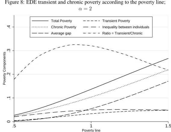
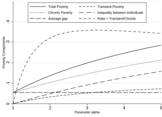
The sensitivity of EDE total, transient and chronic poverty to the choice of poverty line and parameter α is shown in Figures 8 and 9 respectively. Total poverty naturally increases both with the poverty line and with α. For α = 2 and a poverty line set to 1.5, total poverty is deemed to be equal in Figure 8 to about 28% of the poverty line — a similar result is obtained in Figure 9 with a poverty line set to 1 and α = 5. The ratio of transient to chronic poverty never exceeds 0.3 and is a non-monotonic concave function of z and α — the ratio increases at first and then falls as the poverty line increases. Increases in low values of z raise transient poverty relatively rapidly initially, but further increases in z generate dominating increases in the average poverty gap and in chronic poverty. Although non-monotonic, the EDE ratio of transient to chronic poverty is much more stable than with the JR approach. Intuitively, the ratio of transient to chronic poverty depends strongly on the magnitude of the ”pool” of the poor; in societies with few poor people, one would expect the ratio of transient to chronic poverty to be large. An increase in the poverty line increases both the average poverty gap and variability in poverty statuses, and this tends to decrease the ratio of transient to chronic poverty.
Similar results are obtained in Figure 9 for changes in α. With α = 1, the cost of transiency in poverty gaps is nil. The ratio of transient to chronic poverty thus necessarily increases as α initially rises. It reaches a peak at α = 3, after which value it stays roughly constant at 0.3. This is again in stark contrast to the JR estimates. The ratio of the cost of within to between individual inequality is also quite stable as α varies, confirming that the magnitude of these two sources of variability in poverty gaps is not very different, with the cost of inequality between individuals being slightly more important.
5 Conclusion
Whether chronic poverty is more or less important than transient poverty, which of these two types of poverty should be a greater priority for policy, and whether policy should differ according to which of chronic or transient poverty is targeted is an object of debate. Quoting from Jalan and Ravallion (1998),
The degree of transient poverty that we find in [our Chinese] data throws open the question as to whether the current emphasis on fight-ing chronic poverty in China through poor-area development pro-grams is appropriate. (...) The exposure to uninsured income risk that
underlies the high transient poverty will probably persist even within successful program areas. Hence, the many poor in non-program ar-eas will not benefit. There is a case for considering more finely tar-geted programs, although not as a means of fighting chronic poverty but rather as a way of stabilizing incomes by making assistance con-tingent on adverse events. (p.356)
Hulme and McKay (2005) take a somewhat different general stance: At present, chronic poverty is still not seen as an important policy fo-cus. This is a significant area of neglect both because a substantial proportion of poverty is likely to be chronic (Chronic Poverty Re-search Centre, 2004), and because it is likely to call for distinct or additional policy responses. (p.2)
This paper clearly does not resolve this measurement and policy debate. We show, however, that the relative magnitude of chronic and transient poverty — and presumably therefore the shape that policy should take — depends on the mea-surement system that is used. In contrast to those of Jalan and Ravallion (1998), this paper’s proposed indices of chronic and transient poverty are 1) monotoni-cally increasing in the usual parameter α of aversion to poverty, 2) money met-ric, 3) and are conceptually comparable to the conventional money-metric indices found in the risk, inequality and social welfare literature. The indices proposed in this paper also allow total poverty to be expressed as a sum of mean poverty and inequality in poverty, and inequality in poverty to be expressed as a sum of between- and within-individual poverty.
For the same usual parameter value and poverty line that are used with the JR approach, the money-metric approach proposed in this paper suggests that tran-sient poverty represents around 23% of total poverty in our Chinese rural data. This is a significant departure from the JR approach, which suggests that transient poverty accounts for around 73% of total poverty. We also see how the ratio of transient to chronic poverty will usually depend strongly on the magnitude of the pool of the poor: in general, the lower the poverty headcount, the greater the ratio of transient to chronic poverty that we should expect. Finally, the paper shows the usefulness of applying bias corrections when using panel data with a relatively modest number t of time periods. The proposed simple bias corrections work well in all of the cases considered. Even for only 2 time periods, the biases of the naive estimators of chronic and transient are reduced by around 50% by the bias
corrections. The biases disappear quickly with t when the corrections are applied (and mostly vanish for t ≥ 6), and these corrections are particularly effective for the estimators of the measurement approach developed in this paper.
6 Appendix
Proof of Theorem 1.
Note first from equations (6), (10), and (13) that
Cα(γα) = Γα(γα) − Γ1(γα) = Γα(g) − Γ1(γα). (34) Using (11) and (12), note also that
ΓT α(g) = n−1 " n X i=1 γα(gi) − γ1(gi) # (35) = Γ1(γα) − Γ1(g). (36)
(Line (36) follows from (2), (7) and (13).) Hence, regrouping terms, we obtain Γα(g) = Γ1(g) + Cα(γα) + ΓTα(g). (37) Details of the derivation of the bias corrections in equations (24) and (27). Taylor-expanding
³ 1 − byi
´α
+around the true value P
∗
α,i, we find that
E ·³ 1 − byi ´α + ¸ = P∗ α,i+ E h −α (1 − yi)α−1+ ³ byi− yi´ (38) + α(α − 1) 2 (1 − yi) α−2 + ³ byi− yi´2 (39) + α(α − 1)(α − 2) 6 (1 − yi) α−3 + ³ b yi− yi ´3 + . . . ¸ (40) Note that E h³
byi− yi´i = 0. Assuming independence across the time observa-tions, we also have that
E ·³ byi− yi´2 ¸ = E "µP jyij t − yi ¶2# (41) = t−2E Ã X j (yij − yi) !2 (42) = t−2E " X j (yij − yi)2 # (43) = t−1var(yij), (44) where var(yij) = R
(y − yi)2dFi(y). A similar result obtains for higher-order terms, e.g., E ·³ b yi− yi ´3¸ = E "µP yij t − yi ¶3# (45) = t−3E·³Xyij − yi ´3¸ (46) = t−2 Z (y − yi)3dFi(y). (47) Hence, a s-order bias-corrected estimator of
³ 1 − byi ´α + is given by c P∗α,i = ³ 1 − byi ´α + (48) − s X m=2 µ t−m+1 Qm l=1(α − l + 1) m! (1 − yi) α−m + Z (y − yi)mdFi(y) ¶ .
E [γα(gi)] =E Ã t−1X j gij !1/α (49) =γα,i+ E£α−1P α(gi)1/α−1 £ Pα(gi) − Pα,i ¤ (50) +α−2(1 − α)P α(gi)1/α−2 £ Pα(gi) − Pα,i ¤2 (51) + α−3(1 − α)(1 − 2α)P α(gi)1/α−3 £ Pα(gi) − Pα,i ¤3i (52) + . . . (53)
This leads to a s-order bias-corrected estimator of γα(gi) of the form b γα,i= γα(gi) − s X m=2 Ã α−mt−m+1 Qm−1 l=1 (1 − lα) m! ¡ γα,i¢1−mα Z ¡ (1 − y)α +− Pα,i ¢m dFi(y) ! . (54) Recall that we assume above that the yij are distributed independently across the time periods j. If the observations were positively serially correlated, for instance, the bias corrections in (48) and (54) above would need to be larger. The usually small value of t can make it relatively difficult, however, to test whether this independence assumption is valid.
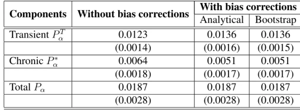
Table 1: JR transient and chronic poverty, with and without bias corrections; α = 2; asymptotic standard errors within parentheses
Components Without bias corrections With bias correctionsAnalytical Bootstrap Transient PT α 0.0123 0.0136 0.0136 (0.0014) (0.0016) (0.0015) Chronic P∗ α 0.0064 0.0051 0.0051 (0.0018) (0.0017) (0.0017) Total Pα 0.0187 0.0187 0.0187 (0.0028) (0.0028) (0.0028)
Table 2: JR transient and chronic poverty, with and without bias corrections, and using censored incomes for chronic poverty; α = 2; asymptotic standard errors
within parentheses
Components Without bias corrections With bias correctionsAnalytical Bootstrap
Transient 0.0083 0.0095 0.0094 (0.0009) (0.0010) (0.0010) Chronic 0.0104 0.0092 0.0093 (0.0021) (0.0020) (0.0020) Total 0.0187 0.0187 0.0187 (0.0028) (0.0028) (0.0028)
T able 3: EDE transient and chronic po verty ,with and without bias corrections; α = 2; asymptotic standard errors within parentheses Components W ithout bias corr ections W ith bias corr ections Analytical Bootstrap A verage gap Γ1 (g ) 0.0545 0.0545 0.0545 (0.0068) (0.0068) (0.0068) Cost of inequality between indi viduals Cα (γα ) 0.0532 0.0491 0.0478 (0.0037) (0.0038) (0.0038) Chronic Γ ∗ (g ) 0.1077 0.1036 0.1024 (0.0095) (0.0093) (0.0092) T ransient Γ T α(g ) 0.0291 0.0332 0.0344 (0.0020) (0.0023) (0.0024) T otal Γα (g ) 0.1368 0.1368 0.1368 (0.0103) (0.0103) (0.0103) 28
Figure 1: The cost of inequality and variability in poverty gaps
g
α ig
1Γ
( )
g
2 1g
Γ
α( )
g
C ( )
αg
P ( )
αg
P ( )
αΓ
1( )
g
Figure 2: Between-indi vidual and within-indi vidual inequality in po verty
g
g
11g
12g
21g
22γ
g
( )
1 1γ
g
( )
1 2γ
g
( )
α 1γ
g
( )
α 2Γ
γ
( )
1 αΓ
g
( )
αΓ
( )
1g
P
( )
g
αFigure 3: Illustrative example with one household i and two periods; gi1= 0.5 − e, gi2= 0.5 + e; α = 2 0 .1 .2 .3 .4 .5 0 .1 .2 .3 .4 .5 e Total Transient Chronic JR Approach 0 .2 .4 .6 .8 0 .1 .2 .3 .4 .5 e Total Transient Chronic EDE Approach 0 .2 .4 .6 .8 1 0 .1 .2 .3 .4 .5
JR Approach EDE Approach
Figure 4: Monte-Carlo simulations of the impact of bias corrections .1 .15 .2 .25 2 4 6 8 10 12 14 16 18 20 22 24 Number of periods (t) Population Without correction Analytical Analytical (uncensored) Bootstrap
JR’s chronic poverty: alpha=2, z=1.5
.52 .53 .54 .55 .56 2 4 6 8 10 12 14 16 18 20 22 24 Number of periods (t)
EDE transient poverty: alpha =2, z=1.5
.05 .1 .15 2 4 6 8 10 12 14 16 18 20 22 24 Number of periods (t)
JR’s chronic poverty: alpha=3, z=1.5
.54 .56 .58 .6 .62 2 4 6 8 10 12 14 16 18 20 22 24 Number of periods (t)
Figure 5: Conditional standard deviation of poverty gaps at different levels of average poverty gaps
0 .05 .1 .15 .2 .25 STD(Gap|Mean gap) 0 .2 .4 .6 .8
Mean gap (8 periods)
1987 1991
Figure 6: JR transient and chronic poverty according to the poverty line; α = 2 1 2 3 4 5 Ratio = Transient/Chronic 0 .02 .04 .06 .08 Poverty Components .5 1 1.5 Poverty line
Total Poverty Transient Poverty Chronic Poverty Ratio = Transient/Chronic
Figure 7: JR transient and chronic poverty according to the parameter α; poverty line=1 2 4 6 8 10 Ratio = Transient/Chronic 0 .02 .04 .06 Poverty Components 1 2 3 4 5 Parameter alpha
Total Poverty Transient Poverty Chronic Poverty Ratio = Transient/Chronic
Figure 8: EDE transient and chronic poverty according to the poverty line; α = 2 0 .1 .2 .3 .4 Poverty Components .5 1 1.5 Poverty line
Total Poverty Transient Poverty
Chronic Poverty Inequality between individuals Average gap Ratio = Transient/Chronic
Figure 9: EDE transient and chronic poverty according to the parameter α; poverty line =1 0 .1 .2 .3 .4 Poverty Components 1 2 3 4 5 Parameter alpha
Total Poverty Transient Poverty
Chronic Poverty Inequality between inidividuals Average gap Ratio = Transient/Chronic
References
[1] Atkinson, A.B. (1970), On the Measurement of Inequality, Journal of
Eco-nomic Theory, vol. 2, 244–263.
[2] Atkinson, A. B., B. Cantillon, E. Marlier and B. Nolan (2002), Social
Indi-cators — The EU and Social Inclusion, Oxford University Press, Oxford.
[3] Bane, M. J., and D. T. Ellwood (1986), Slipping into and out of Poverty; The Dynamics of Spells, Journal of Human Resources, vol. 21, 1–23.
[4] Baulch, B. and J. Hoddinott (2000) (eds.), Economic Mobility and Poverty
Dynamics in Developing Countries, London: Frank Cass.
[5] Benjamin, D., L. Brandt and J. Giles (2005), The Evolution of Inequality in Rural China, Economic Development and Cultural Change, vol. 53(4), 769-824.
[6] Bourguignon, F., Goh, C.-c., and Kim, D. I. (2004), Estimating Individual Vulnerability to Poverty with Pseudo-Panel Data, Washington DC, World Bank.
[7] Breen, Richard, and Pasi Moisio (2003), Poverty Dynamics Corrected for Measurement Error, Journal of Economic Inequality, vol. 2, 171–191. [8] Calvo, C., and S. Dercon (2005), Measuring Individual Vulnerability, paper
presented at the International Conference on The many dimensions of poverty, International Poverty Centre, Brasilia, Brazil, 29–31 August. [9] Chaudhuri, S., J. Jalan, and A. Suryahadi (2002), Assessing Household
Vul-nerability to Poverty from Cross-sectional Data: A Methodology and Estimates from Indonesia, Columbia University, Discussion Paper 0102-52.
[10] Chen, S. and M. Ravallion (1996), Data in Transition: Assessing Rural Liv-ing Standards in Southern China, China Economic Review, vol. 7(1), 23-56.
[11] Christiaensen, L. and K. Subbarao (2004), Toward an Understanding of Household Vulnerability in Rural Kenya, World Bank Policy Research Working Paper 3326.
[12] Chronic Poverty Research Centre (2004), The Chronic Poverty Report 2004–
05, Institute for Development Policy and Management, University of
[13] Cruces, Guillermo, and Quentin Wodon (2003), Transient and chronic poverty in turbulent times: Argentina 1995-2002, Economics Bulletin, vol. 9, #3, 1–12.
[14] Foster, J. E., J. Greer and E. Thorbecke (1984), A Class of Decomposable Poverty Measures. Econometrica, vol. 52, 761–765.
[15] Gaiha, R. (1988), Income Mobility in Rural India, Economic Development
and Cultural Change, vol. 36, 279–302
[16] Gaiha, R. (1989), Are the Chronically Poor also the Poorest in Rural India?,
Development and Change, vol. 20, 295–322.
[17] Giles, J. and K. Yoo (2005), Precautionary Behavior, Migrant Networks and Household Consumption Decisions: An Empirical Analysis Using Household Panel Data from Rural China, mimeo, Michigan State Uni-versity.
[18] Gustafsson, B. and S. Li (2002), Income Inequality within and across Coun-ties in Rural China, 1988 and 1995, Journal of Development Economics, vol. 69(1), 179-204.
[19] Hulme, D., and A. McKay (2005) Identifying and Measuring Chronic Poverty: Beyond Monetary Measures, paper presented at the Interna-tional Conference on The many dimensions of poverty, InternaInterna-tional Poverty Centre, Brasilia, Brazil, 29–31 August.
[20] Jalan, J. and M. Ravallion (1998), Transient Poverty in Postreform Rural China, Journal of Comparative Economics, vol. 26, 338-357.
[21] Jalan, J. and M. Ravallion (2002), Geographic Poverty Traps? A Mi-cro Model of Consumption Growth in Rural China, Journal of Applied
Econometrics, vol. 17, 329-346.
[22] Jarvis, Sarah, and Stephen P. Jenkins (1997), Low Income Dynamics in 1990s Britain, Fiscal Studies, vol. 18, 123–142.
[23] Kamanou, G., and J. Morduch (2004), Measuring Vulnerability to Poverty, chapter in Dercon, S. (ed.), Insurance against Poverty, Oxford University Press, Oxford.
[24] Khan, Azizur R. (2004), Growth, Inequality and Poverty in China: A Com-parative Study of the Experience Before and After the Asian Crisis, Is-sues in Employment and Poverty Discussion Paper 15, ILO, Geneva.
[25] Kolm, S. C. (1969), The Optimal Production of Justice, H. Guitton and J. Margolis.
[26] Kurosaki, T., (2006), The Measurement of Transient Poverty: Theory and Application to Pakistan, forthcoming in Journal of Economic Inequality. [27] Ligon, E., and L. Schechter (2003), Measuring Vulnerability, The Economic
Journal, vol. 113, C95–C102.
[28] Lipton, Michael, and Martin Ravallion (1995), Poverty and Policy, in Jere Behrman and T. N. Srinivasan (eds.), Handbook of Development
Eco-nomics, vol. III, North Holland, Amsterdam.
[29] Park, Albert (2005), ”Risk and Household Grain Management in Developing Countries,” The Economic Journal (in press).
[30] Ravallion, M. (1988), Expected Poverty under Risk-Induced Welfare Vari-ability, The Economic Journal, vol. 98, 1171–1182.
[31] Ravallion, M. and S. Chen (2005), China’s (Uneven) Progress Against Poverty, Journal of Development Economics (in press).
[32] Rendtel, Ulrich, Rolf Langeheine, and Roland Bernsten (1998), The Estima-tion of Poverty Dynamics Using Different Household Income Measures,
Review of Income and Wealth, vol. 44, 81–98.
[33] Suryahadi, A., and S. Sumarto (2003), Poverty and Vulnerability in Indone-sia Before and After the Economic Crisis, AIndone-sian Economic Journal, vol. 17, 45–64.
[34] World Bank, (2001), World Development Report 2000/2001 — Attacking Poverty, New York, Oxford University Press.