Modelling the tactical decisions for open-pit mines

lamsade

LAMSADE

Laboratoire d’Analyse et Modélisation de Systèmes pour

l’Aide à la Décision

UMR 7243

Février 2017

Modelling the tactical decisions for

open-pit mines

A. Azzamouri, P. Fénies, F. Fontane, V.Giard

CAHIER DU

380

Modelling the tactical decisions for open-pit mines

Ahlam Azzamouri

a,b

, Pierre Fénies

a,b

, Frédéric Fontane

a,c

, Vincent Giard

a,d

a_{EMINES, University Mohammed VI Polytechnique, 43140 Ben Guerir,}

Morrocco

b_{Université Paris Ouest, 92001 Nanterre, France}

c_{Mines-ParisTech, PSL Research University, 75006 Paris, France} d _{Université Paris-Dauphine, PSL Research University, CNRS,}

LAMSADE, 75016 Paris, France

ahlam.azzamouri@emines.um6p.ma, azzamouri.ahlam@u-paris10.fr, pierre.fenies@emines.um6p.ma, pfenies@u paris10.fr,

fredéric.fontane@emines.ump6.ma, frederic.fontane@mines-paristech.fr,

vincent.giard@emines.um6p.ma, vincent.giard@dauphine.fr

Abstract.: Open-pit deposits are often characterized by a stack of layers of different geological

nature. Some layers are worthless while the ore of the others is of a varying economic value depending on grade. To reach a layer, it is necessary to have first removed the upper layers above the extraction zone. This action results in uncovering the layer in this particular place and in facilitating access to the layers below. This process involves a series of 2 to 7 operations; each one is performed by a machine, some of which are able to perform up to 3 different operations. Ensuring the consistency of mining extraction scheduling over a few months, in order to meet known or forecast demand, is a challenging task. A mining extraction model based on mathematical programming has been proposed but it is hardly usable due to its size. A Discrete Events Simulator modelling is currently being tested to measure the impact of dynamic rules used to allocate the machines and select the target mining areas.

Keywords: optimization, simulation, planning, scheduling, open-pit mining

I. Introduction

This article analyzes the problems posed by tactical decisions related to ore extraction in an open-pit mine, taking the OCP mine as an example.

We start by defining problem characteristics based on a non-ambiguous formalization (Section II) suitable for a linear programming model presented in Section IV, after a brief literature review (Section III). This formalization results shows that the problem is too complex to be solved by this method. We go on to proposing (Section V), a modelling/simulation of the decisional problems using a Discrete Events Simulator. This approach is currently being tested at the Ben Guerir mine.

II. Problem definition

Extraction is a continuous process and the decisions taken by OCP relate to processing of

deposit parcels (OCP’s parcels are of 40 m by 100 m  4000 m2 rectangles). The

decisions to be taken relate to: i) the choice of parcels to be processed knowing that operations are already underway in a number of parcels; ii) the allocation of the machines

available to perform these operations, some of these machines being versatile. Two important points must be noted:

 This is clearly a tactical decision matter, as completion of these operations will last anywhere between several tens of hours to a few hundred hours (the final operation of ore loading onto a truck being the only one to last only a few hours). In addition, one excludes from the decisional scope such set of decisions as determination of vehicle routes, which are related to the choice of parcels to be processed and accordingly are part of the operational scope.

 The problem is posed in terms of satisfying known or forecast demand and thus relates to medium-term scheduling. Most of the papers proposing a mining extraction model (see Section III) seek to develop a production program irrespective of any explicit demand constraint, where the proposed output is implicitly sold according to predetermined terms and conditions. In such a case, one no longer deals with a scheduling problem (which has to do with satisfaction of a given demand) but rather with a strategic planning issue.

Let us now formalize the problem under consideration.

The deposit area is made up of P panels (p 1..P, and we shall focus on a single panel

to illustrate the problem). The panels are deemed to share homogeneous geological characteristics: same number C_p of layers in panel p, (C_p 18, as in the example of

table 1); each layer c_p (c _p 1..C )_P has the same height h

p

c (value shown in column 3

of table 1) and the same geological characteristics taken from the set of the homogeneous geological characteristics pertaining to the deposit (see column 1 of table 1). Some of

these layers are economically worthless; in our example, J 10 from C_p18 layers

corresponds to 10 grades (j 1..J) of phosphate, while the others correspond to “waste”.

The phosphate layers correspond to the layers of table 1, for which only the two last basic operations apply.

Table 1. The longitudinal view

The processing of each layer c_p of a parcel of panel p involves a sequence of basic

operations (o 1..7) as listed in table 2, some of which are irrelevant to certain layers.

Table2. Basic operations o

A chronological order i_p (i _p 1..I_p, with I_p 60 in our example) is defined for the

basic operations that are actually carried out, from the very first basic operation on the first layer to the final basic operation performed on the last layer. We call chronological

operations, those operations which are listed in columns 4 to 10 of table 1. Table 3 shows

the numbers i_p for these chronological operations along with the number of the

corresponding layer c_p and the number for the corresponding basic operation o. One

notes κ

p

i the number of the layer associated with chronological operation ip and i_p,

its basic operation number.

One also notes



_pj the number of the chronological operation corresponding to basic

operation 7 (ore loading) in layer κ

pj

 corresponding to quality j in panel p (e.g. _1,414

Number 1 Number 2 Number 3 Number 4 Number 5 Number 6 Number 7 Levelling /

Drilling Drilling Blasting

Levelling /

Stripping Stripping Stacking Loading Recouvrement Sillon B 1 7.5 1 2 3 4 5 Sillon B 2 0.9 6 7 Intercalaire SB/SA2 3 6.57 8 9 10 11 12 Sillon A2 4 3.43 13 14 Intercalaire SA2/C0 5 11.75 15 16 17 18 19 Couche 0 6 0.81 20 21 Couche 1 7 1.5 22 23 Intercalaire C1/C2 Sup 8 3 24 25 26 27 28 Couche 2 supérieure 9 1.68 29 30

Intercalaire C2 Sup/C3 Sup 10 4.69 31 32 33 34 35

Couche 3 supérieure 11 0.85 36 37 Couche 3 inférieure 12 0.72 38 39 Intercalaire C3 Inf/C4 13 1.24 40 41 42 43 44 Couche 4 14 1.44 45 46 Intercalaire C4/C5 15 4.65 47 48 49 50 51 Couche 5 16 2.75 52 53 Intercalaire C5/C6 17 3.4 54 55 56 57 58 Couche 6 18 0.65 59 60 Layer number Level height

Elementary operations of waiste extraction Elementary operations of Phosphate exploitation

Level Basic operation name Basic operation number

Levelling / Drilling 1 Drilling 2 Blasting 3 Levelling/ Stripping 4 Stripping 5 Stacking 6 Loading 7 Waste Phosphate (Removal)

where the panel characteristics correspond to that of table 1). Then, we note

p

c

 the first

chronological operation performed on layer c_p and

p

g

 , the last chronological operation

performed on that layer (e.g., ₃ 8

p c  _  and ₃ 12 p c  _  , according to table 1).

From then on, it will be supposed that the other panels of the deposit contain a subset of these 18 layers, the height of a layer being different from one panel to another and with possibly missing layers.

Table3. Chronological order i_p

Each basic operation is carried out by a machine from of a heterogeneous fleet park of

M machines (m 1..M). Some machines may perform one, two or three of these basic

operations (for example, a D9 bulldozer can perform operations 1, 4 and 6), at different

costs and operating times for the same basic operation. The Boolean _om value is 1 if

machine m can perform basic operation o and 0, in the contrary case. When dealing with chronological operations, addressing is indirect and leads to work with

i pm



 .

Panel p is split into parcels having the same surface area S_p and having the same geological structure. Volume v

p

c of layer κi_p below parcel cp, associated with the next

chronological operation i_p to be performed, is generally called “block” in the literature;

it directly results from its surface S and its height h

p

c ; a parcel therefore is a stack of

blocks and, in the following pages, the word ‘parcels’ refers to the open-air blocks of this parcel (accessible for processing). Based on the average performance of the machines in the fleet able to perform operation o (and thus

p

i

 ), one deduces the average operating

time θ

i p

 of the basic operation, recorded in table 4 (unit: hour). This yields table 5 in

Chronological number ip Level number cp Basic operation Number o 1 1 1 2 1 2 3 1 3 4 1 4 5 1 5 6 2 6 7 2 7 8 3 1 9 3 2 10 3 3 11 3 4 12 3 5 13 4 6 14 4 7 … … … 54 17 1 55 17 2 56 17 3 57 17 4 58 17 5 59 18 6 60 18 7

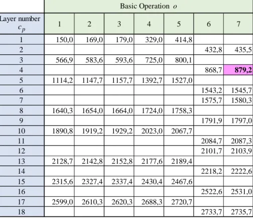
which the processing time for these basic operations are incremented. This last table serves to measure extraction process inertia, since the last ore layer is only accessible after 2,720.7 hours, and even so, under the unrealistic assumption that no time is lost between two successive chronological operations. On the other hand, formulating the problem using a linear program, one will have the exact processing time θ

i pm

 for

operation o by machine m, yielding an hourly input rate of ρ v_κ / θ

i_pm i_p i_pm

   .

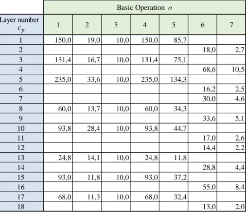
Table 4. Average processing times θ

i p

 of execution of the basic operations

p i  on parcel c_p of panel p Layer number 1 2 3 4 5 6 7 1 150,0 19,0 10,0 150,0 85,7 2 18,0 2,7 3 131,4 16,7 10,0 131,4 75,1 4 68,6 10,5 5 235,0 33,6 10,0 235,0 134,3 6 16,2 2,5 7 30,0 4,6 8 60,0 13,7 10,0 60,0 34,3 9 33,6 5,1 10 93,8 28,4 10,0 93,8 44,7 11 17,0 2,6 12 14,4 2,2 13 24,8 14,1 10,0 24,8 11,8 14 28,8 4,4 15 93,0 11,8 10,0 93,0 37,2 16 55,0 8,4 17 68,0 11,3 10,0 68,0 32,4 18 13,0 2,0 Basic Operation o p c

Table 5: Cumulated processing times 1 θ p p i_{p p} i_p i i i        



of parcel c_p in panel p.

So far, we looked at any parcel of panel p which has N_p parcels referred to as n_p.

From now on, since the decisions concern operations to be carried out on a block accessible from a particular parcel, we shall replace the Subscript of the chronological

operation i_p by the new index

p

n

i to target the block of layer κ

p

i of parcel np of panel p concerned by this chronological operation i_p (this last index remaining valid when relating to an unspecified parcel of panel p).

Each extracted j ore, obtained at the end of the 7th basic operation of layer j (which

corresponds to the basic operation



_pj) is stored in a storage section j having a capacity

of IMax_jt . This capacity, defined at the end of each time period t (t 1..T), varies on the

selected horizon but the dynamics of this change is irrelevant to our analysis. Forecast

demand D_jt for j ore is met through outflows from the inventory of j quality. In fact,

demand for J 10 ores does not correspond to actual final demand. The “primary” J ores

are blended to produce the 5 different ore grades that are required by the downstream supply chain. The problem of defining the blending formula is also irrelevant to this paper (and the latter varies according to change in j inventory levels; see Azzamouri et Giard 2017) and we shall assume that demand for the primary ores is known.

Inventory j receives production P_jt resulting from the set of tactical decisions

reviewed in the next two sections. If one notes I_jt the inventory of ore quality j at the end of period t, the initial inventory being supposed known, the decisions to be taken (in

Layer number 1 2 3 4 5 6 7 1 150,0 169,0 179,0 329,0 414,8 2 432,8 435,5 3 566,9 583,6 593,6 725,0 800,1 4 868,7 879,2 5 1114,2 1147,7 1157,7 1392,7 1527,0 6 1543,2 1545,7 7 1575,7 1580,3 8 1640,3 1654,0 1664,0 1724,0 1758,3 9 1791,9 1797,0 10 1890,8 1919,2 1929,2 2023,0 2067,7 11 2084,7 2087,3 12 2101,7 2103,9 13 2128,7 2142,8 2152,8 2177,6 2189,4 14 2218,2 2222,6 15 2315,6 2327,4 2337,4 2430,4 2467,6 16 2522,6 2531,0 17 2599,0 2610,3 2620,3 2688,3 2720,7 18 2733,7 2735,7 Basic Operation o p c

addition to those relating to IMax_jt ) must meet constraint (1), which is a conservation-of-flow constraint. 0 _{1 1} , IMin_{j j} t t _jt t tD_jt IMax_jt , t t I __ P _ __{ } j t  







  (1)

This relation excludes any withdrawal from safety stock IMin_j and provides that

available capacity IMax_j for the periods t 1..T shall not be exceeded (T having to be sufficient to enable extraction of the entire deposit).

In practice, an insufficient storage space can be remedied with provisional storage, followed by a return to the normal storage when space becomes available, but these operations are without added-value (process described at the bottom of figure 1).

For technical reasons discussed in section III, each block of parcel n_p of panel p is

included in a group g_p (g _p 1..G )_p of R

p

g contiguous parcels (rg_p=1..Rg_p)

belonging to the same layer, corresponding to the break-up into “bench-pushbacks” of the set of all blocks included in a panel (as described in figure 2d). We note

g p

r

i the

number of the chronological operations corresponding to a basic operation performed on

this block (for example, for layer 3 the first basic operation is o  , corresponding to 1

chronological operation 8 in table 1). These groups are subject to relations of precedence

described by Boolean parameter ψ 1 2

p p

g g = 1 where the processing of the group

2

p

g blocks

may only occur after processing of group g blocks. 1_p

This description of the problem matches the decisional practices observed on a tactical level and rests on a discretization of extraction processes whose decisional granularity is at item level, ie the upper available block layer of a parcel, including machinery suitable to perform the relevant basic processing operations. In this context, one can draw up a model of the production process and decisions using mathematical programming (section IV) or Discrete Events Simulation (section V). Before moving on to this, let us present a literature review.

III. Literature Review

Since the 1960s, a number of research papers have dealt with the planning of ore mining in an open-pit mine, based on simulation and/or optimization. These articles were located

on the bib.CNRS documentary metabase (https://bib.cnrs.fr/category/faq-en/) covering

several tens of thousands of scientific journals, using “Open-pit mining or Open-pit mine” and “scheduling or planning” as key words on the abstracts.

The in-depth analysis of the scientific articles identified shows that open-pit mine planning is addressed along two lines: the long term and the medium term. The analysis of the long-term articles (§III.1) is valuable not only to understand the framework for medium- and short-term planning (§III.2), but also because long-term planning relies heavily on scheduling mechanisms. Please refer to §III.3 for our synthetic analysis grid.

III.1 Long-term planning for an open-pit mine

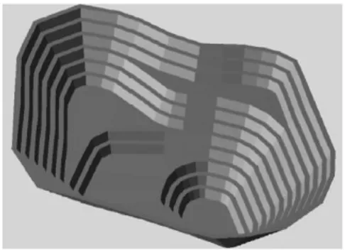
Most scientific articles in this time horizon refer to scheduling or planning but, in fact, deal with the issue of open-pit mine design with a view to structuring the deposit and optimizing its profitability. Such open-pit mine design effort mainly consists in defining, from a geological discretization of the ore body model, the three-dimensional envelope of the deposit which is worth exploiting (“Ultimate pit limits”), and its break up into extraction units called pushbacks. The latter consisting in a set of blocks forming a mini-pit (see Figure 1), considered as a relatively standalone operating entity relevant for medium-term planning purposes. They are also used for long-term economic assessment purposes using discounting techniques.

Figure 1. A 3D view of the second pushback in the Chadormalu iron ore mine

(Gholamnejad et al. 2012)

A summary of the planning stages of the open-pit mine as defined by Chicoine et al. (2009) is set forth below:

 Geological ore body discretization: This stage consists in preparing a discretized model of the deposit by splitting the mine into blocks of equal size, each of which is assigned an estimated tonnage and mineral grades (Journel and Huidbregts 1978, Isaaks and Srivastava 1989).

 Slope angle computations: This phase aims to define the extraction angles (ensuring pit stability) depending on rock structure (faults, shears, etc.), location, depth, within a defined maximum angle. It is based on the precedence relations between blocks, such that the blocks immediately above the block to be extracted must be within the required angles for the slope of the wall (Hustrulid et al. 2000).

 Economic block model: This phase consists in computing, based on tonnage and grade information, an estimated profit for each block in the model, which is dependent on the path followed by the block after extraction.

 Obtaining the three-dimensional envelope of the part of the deposit to be extracted: This phase consists in delimiting the three-dimensional envelope of the ultimate pit limit to be extracted, following the resolution of the ultimate pit limit problem (envelope shown in the cut of Fig. 2a). Lerchs and Grossman (1965) are the first researchers to have proposed an algorithm to solve this problem, successfully implemented by Whittle (1999) Many authors went on to develop their own approach to it.

 Determining a mining sequence: This stage consists in defining a set of nested pits (figure 2a), where the blocks of a pit are only accessible after the blocks of the pits that it surrounds have been removed.

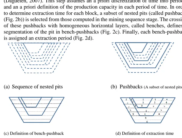
strategic planning. This involves deciding which blocks should be extracted, when they should be extracted, and how the extracted blocks should be processed (Dagdelen, 2007). This step assumes an a priori discretization of time into periods, and an a priori definition of the production capacity in each period of time. In order to determine extraction time for each block, a subset of nested pits (called pushbacks (Fig. 2b)) is selected from those computed in the mining sequence stage. The crossing of these pushbacks with homogeneous horizontal layers, called benches, defines a segmentation of the pit in bench-pushbacks (Fig. 2c). Finally, each bench-pushback is assigned an extraction period (Fig. 2d).

(a) Sequence of nested pits (b) Pushbacks (A subset of nested pits)

(c) Definition of bench-pushback (d) Definition of extraction time

Figure 2. A production plan scheduled by pushbacks (Chicoisne et al. 2009).

The scope of the open-pit mine scheduling problem and its combinatorial nature make it an NP-complex problem where it is difficult to obtain an optimal solution. Most of the research carried out on this subject has focused on designing new methods, algorithms and heuristics (Newman et al. 2010) and provides a valuable overview of the techniques used to solve mine planning problems. Espinoza et al. (2012) draw up a library of open-pit mining problems and associated research) to enhance problem-solving performance and efficiency. Other authors sought to introduce model extensions (for example: Moreno

et al. (2016) for taking stockpiling into account, and Espinoza et al. (2012) to cover

different destinations of mined ore) without entering into the specificities of the mining industry.

Based on this analysis, one can deduct that long-term mine planning serves to define the elements (bench-pushbacks) to be extracted on the life-of-mine horizon but that the detailed scheduling of blocks within each bench-pushback, taking into account all the operational constraints (machines, operations, demand, ...) does not feature at this stage. Thus, an understanding of long-term planning is essential to understand the objective and scope of the integrated modelling in this type of planning, which has led us to analyze medium-term planning (from a few months to a year).

III.2 Open-pit Mine Medium-term extraction planning

few months to address actual or forecast demand and subject to the long-term planning decisions. Concretely, it is designed to draw up a schedule of the blocks to be extracted and the allocation of machinery to meet demand as defined by delivery schedules in terms of qualities and quantities, and to do so in a cost-effective way. This process is performed periodically (rolling planning) to take into account changes in demand, availability of productive resources and mineral characteristics.

A number of articles claiming to address planning objectives in fact merely deal with operational problems with finer granularity (definition of truck routes, etc.).

Our bibliographical research shows that there is a lack of papers addressing medium-term planning. This can be partly explained by the lack of interest in medium-medium-term planning for stock-producing mining companies. Another possible reason is the daunting and complex nature of these scheduling problems. We note that, dedicated modelling of mining operations (drilling, blasting, stripping, ...) is mostly ignored in the literature (L’Heureux et al. 2013) and that management of the allocation of resources as they become available is almost exclusively limited to ore loading and transportation (Fioroni

et al. 2008). And where this point is addressed for other operations, the heterogeneity and

multi-purpose nature of the equipment are barely taken into account.

III.3 Selected analytical grid

A thorough analysis of these articles was carried out on the basis of the criteria listed below; table 6 summarizes this analysis.

 Block Characteristics. All the papers reviewed break mineral deposits down into superposed strata (layers), each made up of a set of blocks; they also take into account the relations of precedence between the block of a stratum and that corresponding to it in the upper adjacent stratum. Additionally, block heterogeneity is a key aspect that should be taken into account in modelling because the heterogeneity of mineral qualities, as in the case of phosphate deposits, induces strong decisional interdependence, obtention of certain minerals being conditioned by extraction, if only partial, of ore from the upper strata. Based on the articles reviewed, we were able to identify three situations where the quality of mined ore (input) was taken into account:

- Single input: in this case, either the mine is limited to producing a single type of ore or that type of ore is the only one considered in the modelling exercise (Meagher et al. 2014b).

- Explicitly heterogeneous inputs: in this case each block is explicitly characterized in the model by a precise grade (Espinoza et al. 2012, Moreno et al. 2016, L'Heureux et al. 2013, Fioroni et al. 2008, Moosavi et al. 2014, Askari-Nasab et

al. 2011, Eivazy et al. 2012).

- Indirectly heterogeneous inputs: several articles implicitly deal with block heterogeneity by computing a profit for each block based on a number of variables, particularly block grade (Chicoisne et al. 2009), Espinoza et al. 2012, Moreno et al. 2016, Moosavi et al. 2014, Meagher et al. 2014a, Amankwah 2011).  Output characteristics. Once the ore has been extracted, it is transported to a stockpile

and/ or a mill. Thus, at the exit point of the assigned destination, three types of outputs related to the nature of input may be identified:

- Single output: obtention of a single output results from the fact that a single input is produced. Additionally, one may implicitly deduce this from the definition of a

constraint that obliges the average grade of output to be greater than or equal to a certain value, without there being any specific constraint on the distinction between outputs, which implies an implicit homogenization of the blocks (Chicoisne et al. 2009, Moreno et al. 2016, Meagher et al. 2014b, Moosavi et al. 2014, Amankwah 2011).

- Multiple outputs with identical segregation: this type of output can only be obtained if the inputs are heterogeneous (explicitly or indirectly). In this case, inputs will be assigned to stockpile or processing plant (sequential or parallel) according to the grade interval required for each destination. Following homogenization, one obtains for each destination an output with grade value equal to the average grade of the ore content on the stockpile or processing plant (Espinoza et al. 2012, L’Heureux et al. 2013, Askari-Nasab et al. 2011, Eivazy et

al. 2012).

- Different outputs: Differentiating outputs from different inputs requires a blending process used to prepare outputs according to different known characteristics using the currently available inputs (Eivazy et al. 2012).

 Type of demand to be met. Mining is carried out to meet defined demand in terms of quality and quantity over the planning horizon. Yet, articles seldom point out that mined ore must satisfy demand defined under long-term contracts with customers (Espinoza et al. 2012) or according to forecasts. Indeed, in the other articles one can implicitly deduct demand from the definition of maximum capacity of the ore to be processed in the plant, which varies over time. This capacity is introduced as a constraint not to be exceeded rather than an objective that extraction operations must achieve. One understands in particular that it is assumed that the extracted quantity must be sold (which amounts to working according to fictitious demand (Moreno et

al. 2016). The problem of the segregation of the demand by qualities sold only arises

in the case of heterogeneity of mined ore; in this case, the variety sold is obtained by mixing (blending) the extracted variety (Fioroni et al. 2008); the fact that the link between production and demand is not set, is an additional factor of complexity.  Breakdown of extraction operations: the mined block processing plant performs a

series of basic operations: some relate only to the blocks containing waste and others, to the ore. Most of the papers distinguish between two types of operation: 1. The mining operation which is seen as a black box (as is the case for most articles dealing with long-term planning). 2. Processing of mined ore (which falls outside the scope of our study). Only L’Heureux et al. (2013), who explicitly deal with short-term planning, take into account the existence of multiple extraction operations to be performed in a certain sequence. The other articles consider block processing as a global operation, which obviously greatly under-estimates the resources required, as these are seen as globally homogeneous. Conversely, one will deduce the existence of multiple operations from the multiplicity of resources mobilized (Chicoisne et al. 2009, Espinoza et al. 2012).

 Heterogeneity of resources mobilized. Each basic operation of the extraction process is carried out by a resource (drilling machine, bulldozer, etc.) which can be specialized in this operation or multi-purpose. Allocating freshly available resources to a block can be a complex decision. Obviously, this is highly simplified in models that consider processing as a single processor. Models that consider block processing involving several pieces of equipment (without disposing of accurate descriptions of their functionalities and uses) tend to treat all machinery as dedicated to a single function (Chicoisne et al. 2009, Espinoza et al. 2012, L’Heureux et al. 2013, Fioroni

mobilized resources have limited capacity, with capacity being defined either i) by maximum handled tonnage (mined waste + ore) in a given period (Moosavi et al. 2014, Askari-Nasab et al. 2011, Eivazy et al. 2012), or ii) in terms of tonnage for each operational resource in a given period (Chicoisne et al. 2009, Espinoza et al. 2012, L’Heureux et al. (2013) [12], Fioroni et al. (2008) [13]),

 Case study: The relevance of a model is always improved when applied to a real case. The explanations obtained in the field clarify a number of underlying hypotheses as well as the contingency of the proposed formulation: the land referred to by Fioroni

et al. 2008, Moosavi et al. (2014), Askari-Nasab et al. (2011) and Eivazy et al. (2012)

concerns an iron ore mine whereas Meagher et al. (2014b) refer to a copper and gold mine. All the other papers are based on a generic presentation of mining without reference to specific land, which limits its scope because open-pit mines do not all share the same features.

 Type of decision. This category generally establishes a distinction between operational, tactical and strategic decisions, which has a strong impact on the level of detail used. As noted above, we have reviewed articles dealing with long-term and short-term planning (L’Heureux et al. 2013, Fioroni et al. 2008, Eivazy et al. 2012). Accordingly, our paper aims to describe, to quite a fine level of granularity and maximum realism, the problem of running a pit mine. Many articles focus on resolution algorithms, rather than on the problem to be solved (which is rarely explicit).

Table 6. Analysis grid of the papers reviewed.

IV Problem formulation through mathematical programming

We are dealing with a set of decisions to be taken simultaneously: i) the production launch

U n iq u e / Mu lt ip le D e d ic a te d / S h a r e d L im it e d / U n li m it e d S p e c if ic / G lo b a l 1 Moosavi et al. 2014 X X X X X X X I L G X X Lagrangian relaxation, Genetic algorithm F1 X 2 Meagher et al. (a) 2014 X X I L G X X

Lerch Grossman Algorithm, Seymour's Parametrized Pit

Limit Algorithm, Network Flow Approaches,

IP formulations, Fundamental Tree,

F1 X

3 Moreno et

al. 2016 X X X X X I L G X X Linear integer model F1 X

4 Espinoza

et al. 2012 X X X X X I M M L G X X Linear programming relaxation F1 X 5 Chicoisne

et al. 2009 X X X I M M L G X X Linear programming relaxation F1 X 6 Meagher et

al. (b) 2014 X X X X X X I X X

The integer program

formulation F1 X

7 Henry

Amankwah2011 X X X L G X X

Lagrangian dual heuristic,

Maximum flow problem F1 X

8 L'Heureux

et al. 2013 X X X X I M M D L S X X Mixed integer programming F2 X 9

Askari-Nasab et 2011 X X X X X X I L G X X

Mixed integer Linear

programming F1 X

10 Eivazy et

al. 2012 X X X X X X I L G X X

Mixed integer Linear

programming F2 X

11 Fioroni et

al. 2008 X X X X X X E M D L S X Programmation mathématique X DES

F2,

F3 X

12 Us 2017 X X X X X X E M M D/P L S X Programmation mathématique X DES F2 X

• Demand definition: I: Implicit. E: Explicit. • Extraction operations: U: Unique. M: Multiple. • Resources mobilized: U: Unique. M: Multiple. D: Dedicated. P: Shared. L: Limited. I: Unlimited. S: Specific. G: Global. • Objective function: F1: Maximize profit. F2: Minimize costs. F3: Maximize ore production per zone.

O p e r a ti o n a l m e th o d n a m e S tr a te g ic T a c ti c a l

Meaning of the notations used in the grid:

Elements taken into account in

modeling Modeling method

O b je c ti v e f u n c ti o n Decision type H o m o g e n iz a ti o n B le n d in g D e m a n d d e fi n it io n E x tr a c ti o n o p e r a ti o n s Mobilized resources Type Capacaity O p ti m iz a ti o n m e th o d n a m e S im u la ti o n Mi ll p la n t P h o sp h a te U n iq u e E x p li c it Production (input)

Use (routing to stock and / or processing unit

(output) Im p li c it ( p r o fi t) S in g le O u tp u t Mu lt ip le o u tp u t w it h sa m e s e g r e g a ti o n O u tp u t d if fe r e n t A r ti c le n u m b e r Author (s) Y e a r Paper Type C a se s tu d y

Type of mine treated

A r ti c le L it e r a tu r e r e v ie w C o a l Ir o n C o p p e r G o ld

dates of chronological operations

p

n

i for parcels n_p of panels p; ii) the allocation of machine m to perform each chronological operation; this allocation defines operating time

ipm



 which determines the termination date of chronological operations

p

n

i .

In this formulation, the binary decision variable 1

n p

i mt

x  is used only if chronological

operation

p

n

i is processed with machine m and is completed at the end of period t (hourly

periods), and 0 in the opposite case. To integrate the restricted multi-purpose use or lack of versatility of the machines and of the fact that the first chronological operations

p

n

q

of parcel n_p of panel p have already been performed at the time of definition of the

problem; these binary variables only exist if I

p p n n p q i  and if 1 i pm    .

Implicitly, the proposed formulation precludes having ongoing operations when first solving the problem but this restriction is easy to lift without increasing problem complexity. It also ignores travel times of machines to reach the next operation site. The corresponding time and costs may be integrated at the cost of a large increase in modelled problem complexity; these additional aspects are also of limited interest in light of the conclusions of this section IV. Let us describe the proposed linear programming model of the problem.

Within planning horizon T of end of exploitation of the deposit, each chronological operation for each parcel must be performed, which is enforced by relation (2). Note that if T is not long enough, implementation of relation (2) precludes a solution from being found. T M 1 1 n_p 1, p t i mt n t m x i     

 

(2) Operation p n

i is completed at the end of the period

n p

i

 , which is the intermediate

variable defined by relation (3).

T M 1 1 , n_p n_p p t i _{t m} txi mt in  

 

_{ }  (3) The precedence constraints between chronological operations are expressed by relation (4) which mobilizes intermediate variable

n p i  . T M 1 _{1 1} , 1 n_p i_p n_p n_p p t i _{t m}  m xi mt i in  _ 

 

_{ }     (4) Operation p n

i is performed during period t if it is completed at the end of period t or

at the latest at the end of period 1

i pm

t_  . It follows that this operation q

p p

n n

i  is

only performed during period t if relation (5) is filled.

1 M 1 1, , q m i p np p p t t m i mt n n m t t x t i              





(5)

During each period t, machine m is available only for one operation, which is reflected in relation (6). 1 I P 1 q 1 1, , m n_p p i_p np n_p n_p t t i p i mt p i t t x t m               

 



(6)

Delivery of j grade ore extracted from parcel n_p of panel p in stock j occurs after basic

operation o 7 (corresponding to



_pj) or in other words, following completion of the

chronological operations performed during periods θ _, 1

n_p pj i_p pj i    m  _  _  to n_p pj i   _ at

the hourly rate ρ

ipm

 . Thus, the feeding P_jt of stock j is given by relation (7), used in

relation (1). , (τ ) P γ , , 1 (τ θ 1) ρ , , in_p pj n_p pj i_p pj in_p pj i_p pjm t p jt _{p t} i mt m P  x j t                      _  _  

 

(7) Finally, one should introduce the group constraints into the scheduling. Relation (4) is required to correctly schedule block processing operations but it does not integrate the

constraint of antecedence between groups ( ψ 1 2 1)

p p

g g

  . Performance of the first

chronological operation 2 p g p r g i  of block 2 p g

r of group g is subject to the last 2_p

chronological operation

1 2 1

gp gp

r r

i i  of all group ancestor blocks g , being performed. 1_p

This is ensured by relation (8).

1 2 1 2 1 2 2 T M 1 _{1 1} , , , ψ 1 r r r g_p i_p n_{p p p p p} g_p g_p g_p t i i i  _{t m}  m xi mt r_g r_{g g g}  _{ }  _ 

 

_{ }     (8)

The objective function of the problem, not discussed, is the sum of production costs (the cost of a basic operation depending on the machine used) and of ore storage.

The size of the linear program defining our problem (about fifty machines, hundreds of boxes, thousands of hours) prevents using it in practice. One can attempt to reduce this size by shortening the temporal horizon (for example, one year of exploitation) and the number of blocks to be processed on the relevant horizon. This reduction involves limiting the value of T in relations (2) and (1) and to address a sub-set of blocks.

To this end, two options are available. The first consists in selecting blocks arbitrarily for processing over the reduced horizon (without guaranteeing problem feasibility), with a risk of degraded performance versus the situation obtaining with a higher value for T. The second option consists in overriding the equality of relation (2) by inequality “”; in this case, the cost reduction induces the lowest possible production levels, a tendency offset by relation (1), corresponding to stock conservation equations, designed to satisfy demand for ore grades; this latter option does not decrease the number of problem binary variables.

From our point of view, these observations imply that the best possible approach to support tactical decisions is to rely on simulation.

V Problem Formulation using discrete events simulation

Modelling mining extraction processes by discrete events simulator (DES) and the related production decisions, rests on the combination of two complementary views of deposit panels:

 The longitudinal view plots the gradual processing of parcels in a panel, from the first

layer to the last one. This gradual transformation of parcel n_p in panel p involves

successive performance of chronological operations I_p (see tables 1 and 3).

 The transversal view deals with the “current state” of deposit parcels at date t, amounting to a “bird’s eye view” snapshot of the deposit. It rests on basic operation

o (table 2). At any date t, one can split the set of parcels in 7 subsets, one per basic

operation; each subset in turn being split into two: the first including parcels undergoing the relevant operation and the second including the remaining parcels. In this context, the modelling of the extraction process rests on 7 sets of parallel heterogeneous processors. Each set is specialized in the processing of one basic operation

o for one parcel of a panel (amounting to operation p n i such as n p i o   ). To be

operative, a processor must mobilize one of the machines m suitable for this operation

(implying



_om1 and thus 1

inpm



  ); these machines, some of which are

multi-purpose, are deemed usable on all parcels. The allocation of machine m to perform operation

n p

i

 leads to processing time θ

inpm

 .

The modelling of the productive system of mining extraction by simulation includes two specific features.

 The first feature is that the productive system is semi-open: there is no inflow of items into the system but there is constant outflow of items (extracted ores, via operation 8, and waste, as illustrated at the bottom of figure 1, corresponding to the “Transport” sub-process). The simulation then ends with depletion of the deposit.

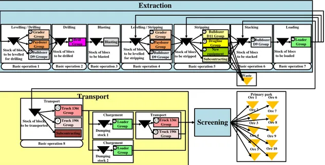
 The other feature flows from the analysis of table 3 describing the series of 60 chronological operations and delivers the “Extraction” sub-process of figure 1. Figure 1 summarizes the mining extraction process model implemented in the DES Simul8. Conventionally, in this diagram, the processor performing operation o on a parcel represents a set of k identical parallel processors mobilizing the same type of machine (identified by the number shown in the processor box in figure 1). When machines with different characteristics perform operation o, these alternatives are represented by as many processors (thus they are duplicated in the figure). Certain machines being able to perform two or three of the basic operations, this is shown in the diagram by a color convention, the alternative processors of one color using the same type of machine.

Figure 3. Modelling of the deposit extraction process.

All extracted layers are normally intended to feed the mechanical processing (screening) plant. Where one of the ore stocks becomes saturated (or the screening plant breaks down) the ore is either moved to a remote dumping stock 1 (implying mobilization of trucks), or in a nearby dumping stock 2 (in which case, the loader which feeds the screening plant may be used). In both cases, such intermediate storage adds no value.

We have noted that this modelling relies on a DES. This class of simulator is designed to model and simulate discrete processes and not continuous processes. The discretization performed by splitting a panel into parcels does not interfere with the modelling of basic operations1 to 7. But downstream, beginning from the basic operation 8, two technical issues arise (which our simulation solves satisfactorily):

 The mass of ore corresponding to ore volume v

p

c extracted from parcel np of layer

p j

c 



by operation

p

n

i is much greater than the capacity of the truck used to

perform operation 8, it being known that the 3 types of trucks have different capacities. To address this, we designed a converter which enables capping truck load to its maximum load capacity (offloading the balance into the upstream stock).  In DES, stock capacity is defined by the maximum number of items it can contain.

The items which are fed into an ore stock don’t all have the same weight due to the heterogeneity of capacity of the truck fleet used to transport them. To solve with this problem, we defined stock capacities in terms of maximum weight: stock capacity is updated with the weight of each outbound item (this aspect falls outside the scope of our paper) and with the weight of each inbound item (provided there is sufficient available space).

Finally, one must deal with the problem posed by the reallocation of the machines that have completed a basic operation. This issue is key for multi-purpose machinery (e.g., bulldozer D9). All parcels waiting to undergo a processing operation and suitable for this equipment are eligible (e. g., D9 bulldozers can perform basic operations 1, 4 and 6). One must then define dynamically in the simulation for each parcel, a priority index addressing two potentially conflicting points of view.

Transport Waste Extraction Chargement Basic operation 6 Stacking Blasting Drilling Levelling / Drilling Grader Group Drill Group Blasting

Levelling / Stripping Stripping

Bulldozer D9 Group Loading Transport Stock of blocs to be levelled for drilling Stock of blocs to be drilled Stock of blocs to be blasted Stock of blocs to be levelled for stripping Stock of blocs to be stripped Stock of blocs to be stacked Stock of blocs to be loaded Stock of blocks to be transported Paydozer Group Bulldozer D9 Groupe

Basic operation 1 Basic operation 2 Basic operation 3 Basic operation 4

Bulldozer D11 Group Dragline Group New equipment Subcontracting Loader Group Truck 136t Group

Basic operation 5 Basic operation 7

Basic operation 8 Screening Dumping stock 1 Loader Group Transport Truck 136t Group Chargement Loader Group Dumping stock 2 Primary park Ore 1 Ore 2 Ore 3 Ore 4 Ore 5 Ore 6 Ore 7 Ore 8 Ore 9 Ore 10 Truck 190t Group Truck 190t Group 3 2 9 4 7 5 2 9 2 3 2 3 12 12 2 Subcontracting Grader Group Paydozer Group Bulldozer D9 Groupe 3 2 9

 The choice of a candidate parcel results in changing the earliest feedings of j ores (resulting from table 5 and from the basic operations already performed on this

parcel). These forecasts, combined with those for demand D_jt for j ores, yield a

priority index for all the candidate parcels. Such calculation of priority indexes also includes the distances from the starting parcel to the destination one.

 This earliest feeding of an ore stock may lead to temporary storage due to insufficient capacity, causing additional handling without added value. This should of course be avoided, although access to certain ores in certain parcels involves extracting ore from other layers before reaching the targeted one. Remember that ore demand is indirect as resulting from quality requirements downstream in the supply chain, thus involving blending in different proportions the ten qualities of extracted ores where different blends can yield the same required quality. This aspect has been left out of the simulation where ore demand is assumed to be known.

Note that we are currently developing the method to calculate the priority indexes.

VI Conclusion

The space-time interdependence of the decisions (parcels to be processed, allocation of the machines) is such that tactical management of deposit extraction is an arduous task which entails costly remedial actions. We have shown that an optimization approach is not adequate. On the other hand, simulation can prove a valuable tool to mine managers but involves developing a relevant system of dynamic priorities to allocate particular pieces of equipment to candidate parcels.

VII References

Amankwah Henry, Mathematical optimization models and methods for open pit mining, Linköping Studies in Science and Technology, Dissertations No. 1396, 2011. Askari-Nasab, H., Pourrahimian, Y., Ben-Awuah, E., and Kalantari, S., Mixed integer

linear programming formulations for open pit production scheduling, Journal of Mining Science, 2011; 47 (3).

Azzamouri, A., Giard, V., Tailored blending definition as a source of flexibility in

controlling mine production, 4th International Symposium on Innovation and

Technology in the Phosphate Industry-SYMPHOS, 2017.

Chicoisne, R., Espinoza, D., Goycoolea, M., Moreno, E., Rubio, E., A new algorithm for the open-pit mine scheduling problem, Operations Research, 200; 60: 517 – 528. Dagdelen, K., Open pit optimization - strategies for improving economics of mining

projects through mine planning, Orebody Modelling and Strategic Mine Planning, Spectrum Series, 2007; 14:125-128.

Eivazy, H. and Askari-Nasab, H., A mixed integer linear programming model for short-term open pit mine production scheduling, Mining Technology, 2012; 121(2): 97– 108.

Espinoza, D., Goycoolea, M., Moreno, E., Newman, A., MineLib: a library of open pit mining problems, Annals of Operations Research, 2013; 206: 93–114.

Fioroni, M. M., Franzese, L. A. G., Bianchi, T. J., Ezawa, L., Pinto, L. R. and Miranda, G. 2008, Concurrent simulation and optimization models for mining planning, Proceedings of the 2008 Winter Simulation Conference (ed. S. J. Mason et al.), 2008.

Gholamnejad, J. and Moosavi, E., A New Mathematical Programming Model for Long-Term Production Scheduling Considering Geological Uncertainty, Journal of the Southern African Institute of Mining and Metallurgy, 2012;112.

Hustrulid, W. A., Carter , M.K., and Van Zyl, D.J.A., Slope stability in surface mining. Society for Mining, Metallurgy, and Exploration, Inc., Litleton, Colorado, 2000. Isaaks, E.H. and Srivastava R.M., Applied geostatistics, Oxford University Press, New

York, USA, 1989.

Journel, A.G. and Huidbregts C.J., Mining Geostatics, Academic Press, San Diego, USA, 1978.

Lerchs, H and Grossman, I.F., Optimum Design of Open Pit Mines, Joint CORS and ORSA Conference, Transactions Canadian Institute of Mining and Metallurgy, Montreal, 1965.

L’Heureux, G., Gamache, M., Soumis, F., Mixed integer programming model for short term planning in open-pit mines, Mining Technology, 2013; 122: 101–109.

Meagher, C., Dimitrakopoulos, R., Vidal, V., A new approach to constrained open pit pushback design using dynamic cut-off grades, Journal of Mining Science, 2014; 50: 733–744.

Meagher, C., Dimitrakopoulos, R., Avis, D., Optimized Open Pit Mine Design, Pushbacks and the Gap Problem—A Review, Journal of Mining Science, 2014; 50: 508-526. Moosavi, E., Gholamnejad, J., Ataee-pour, M., Khorram, E., A hybrid augmented

Lagrangian multiplier method for the open pit mines long-term production scheduling problem optimization, Journal of Mining Science, 2014; 50: 1047–1060. Moreno, E., Rezakhah, M., Newman, A., Ferreira, F., Linear models for stockpiling in open-pit mine production scheduling problems, European Journal of Operational Research, 2016.

Newman, A. M., Rubio, E., Caro, R., Weintraub, A., A review of operations research in mine planning, Interfaces, 2010; 40(3): 222–245.

Whittle, J., A decade of open pit mine planning and optimization - The craft of turning algorithms into packages, APCOM’99 Computer Applications in the Mineral Industries 28th International Symposum, Colodado School of Mines, Golden, Co, USA, 1999.

VIII Table of notations Indexes

J Subscript of ore quality (j 1..J)

T Subscript of time period (t 1..T)

P Subscript of panel (p 1..P)

p

c Subscript of panel p layer (c _p 1..C )_P

p

n Subscript of a parcel in panel p (n _p 1..N )_p

p

g Subscript of parcel group in panel p (g _p 1..G )_p

p

g

r _{Subscript of a bloc in group} g_p ( =1..R )

p p

g g

r

o Subscript of basic operations (o 1..7)

p

panel p

p n

i Subscript of chronological operations(i _p 1..I )_p performed in parcel n_p of

panel p ( κ , ) n_p n_p i i  g p r

i _{Subscript of chronological operations performed on block}

p g r of group g_p ( .. ) g_p p p r g g i   m Subscript of machines (m 1..M) Parameters q p

n Number of chronological operations already performed on parcel np

of panel p h

p

c Height of layer cp of panel p

S_p Surface area of a parcel of panel p

v

p

c Volume of layer cp of panel p

κ

p

i Number of the layer associated with chronological operation ip

p i

 Number of the basic operation associated with chronological

operation i_p pj



Number of chronological operation associated with basic operation 7

consisting in extracting j grade from panel p

p

g

 Number of the first chronological operation performed on a block of

group g_p.

p

g

 Number of the last chronological operation performed on a block of

group g_p.

1 2

ψ

p p

g g Boolean = 1 if blocks of group g can be only processed if all the 2p

blocks of group g have previously been processed. 1_p

om



_,

i pm



 Boolean = 1 if machine m can perform basic operation o and

therefore the basic operation

p i  associated to chronological operation i_p θ i p

 Average processing time of basic operation

p i  i p   1 θ p p i_{p p} i_p i i i        



θ i pm

 Processing time of basic operation

p i

 processed by machine m

ρ

i pm

 Hourly flow rate of basic operation

p i  by machine m κ (ρ v / θ ) i_pm i_p i_pm   

IMin_j Safety stock of of j grade ore

IMax_jt Maximum available capacity of j grade stock at the end of period t

D_jt Demand for j grade ore in period t

0

I_j Initial stock of j grade ore used in optimization and simulation

models

Variables

n p

i mt

x Binary variable = 1 if the chronological operation

p n

i is processed by

machine m and is completed at the end of period t Order variable

I_jt Stock of j ore at the end of period t

Intermediate variable (relation 1, using relation 7) n p

i

 Period of completion of operation

p n i

Intermediate variable (relation 3)

jt

P Supply of j ore during period t