Complex lot Sizing problem with parallel machines and setup carryover

de

PSL Research University

Préparée à

-Dauphine

Soutenue le

par

cole Doctorale de Dauphine

ED 543

Spécialité

Dirigée par

Complex lot Sizing problem with parallel machines and

setup carryover

28.11.2017

Xueying SHEN

Virginie GABREL

Université Paris-Dauphine Mme Virginie GABREL

Université Paris-Dauphine M. Fabio FURINI

M. Filippo FOCACCI DecisionBrain

M. Stéphane DAUZERE-PERES Ecole des Mines de Saint-Etienne

Mme Safia KEDAD-SIDHOUM Université Paris 6

M. Chengbin CHU ESIEE Paris

M. Roberto WOLFLER CALVO Université Paris 13

M. Vincent GIARD

Université Paris-Dauphine, EMINES

Informatique

In this thesis, we study two production planning problems motivated by challenging real-world applications.

In the first part of this manuscript, a production planning problem for an apparel manufacturing company is studied and an optimization tool is developed to tackle it. We propose a decomposition framework composed by an aggregated model and a de-tailed model, which are solved in sequence. The aggregated problem is shown to be the bottleneck of the approach, which corresponds to a complex capacitated lot sizing problem with setup carryover, parallel machines, production time windows, backlogging and lost sales. This problem is shown to be NP-hard even without the setup costs. Several Mixed Integer Programming (MIP) formulations are proposed and compared from a theoretical and a computational point of view. Moreover, several constructive and local search heuristics are developed to find good quality solutions for large scale instances. We propose two sets of benchmark instances to evaluate the performances of the models and the heuristics. Thanks to extensive computational tests, we showed that the constructive heuristic (called First-Solution Heuristic) together with a Fix&Optimize algorithm is able to compute the best solutions in terms of optimality gap. Finally, the whole production planning approach is presented and its performance is analyzed.

In the second part of this manuscript, a restricted version of the capacitated lot sizing problem with sequence dependent setups is studied, where the setup sequences for each time bucket have to follow the order of a given sequence. Compared to the capacitated lot sizing problem with sequence dependent setup, the new model reduces the number of candidate setup sequences from O(n!) to O(n2n) where n is the number of products. This problem is shown to be NP-hard. A special case with only two possible setup values is studied and we prove that also in this case the problem remains NP-hard. Moreover, product-oriented and sequence-oriented MIP formulations are developed. A column gen-eration heuristic is also proposed based on the sequence-oriented formulations. Finally, we perform computational tests to evaluate their respective computational performance.

— The Wrong Trousers, Aardman Animations, 1993

I would like to thank my supervisors Dr. Virginie Gabrel, Dr. Fabio Furini, Dr. Filippo Focacci and Mr. Daniel Godard. You gave this wonderful chance to pursue my study and guide me through my research with tremendous patience and profound knowledge. Without your supervision and constant help, this dissertation would not have been possible.

Deep thanks are owed to Dr. St´ephane Dauz`ere-P´er`es, I would not have accomplished what I have without your insight and expertise that greatly assisted the research. My deep gratitude to the thesis committee member Dr. Safia Kedad-Sidhoum, Dr. Chengbin Chu, Dr. Roberto Wolfler Calvo and Dr. Vincent GIARD, for your precious time and valuable comments on this work.

I would like to express my appreciation to all of my colleagues, it is a great pleasure to work with such cheerful and talented people like you. Special thanks to Kiat Shi Tan, Issam Mazhoud, David Gravot, Giulia Burchi and D´esiree Rigonat that you generously shared your experience and knowledge with me and accompanied me through my PhD. Finally, I would like to express my sincere gratitude to my parents, my husband Alexandre Menif and my dear friends, my deep love to all of you.

Abstract ii

Acknowledgments v

Contents vi

List of Tables viii

List of Figures x

1 Industrial and Scientific Context 1

1.1 Introduction . . . 2

1.2 Production Planning: Lot Sizing Problem . . . 4

1.3 Production Planning in An Apparel Manufacturing Application . . . 12

1.3.1 An Apparel Manufacturing Application . . . 13

1.3.2 Production Planning Problem Modeling . . . 16

1.4 Contributions . . . 17

2 Complex Capacitated Lot Sizing Problem: Formulations and Bench-marks 18 2.1 Problem Definition . . . 19

2.2 Literature Review . . . 22

2.3 MIP Formulations . . . 28

2.4 Benchmark Instances . . . 35

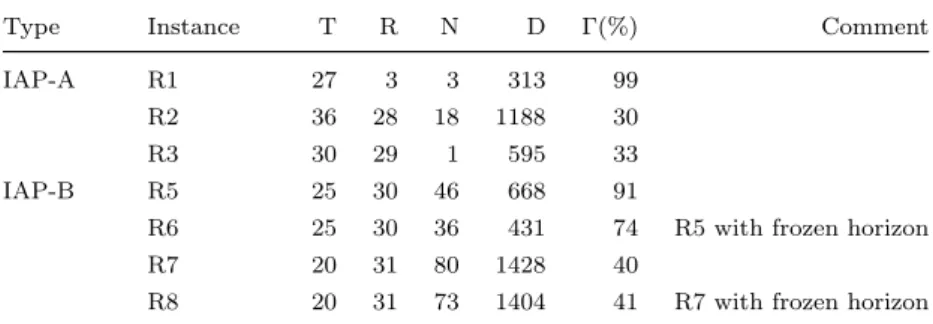
2.4.1 Benchmark IAP: Real-World Instances and Data Analysis . . . 35

2.4.2 Benchmark IRG: Pseudo-Randomly Generated Instances . . . 43

2.5 Empirical Evaluations . . . 48

2.5.1 MIP Formulation Comparison Considering Setup Cost . . . 48

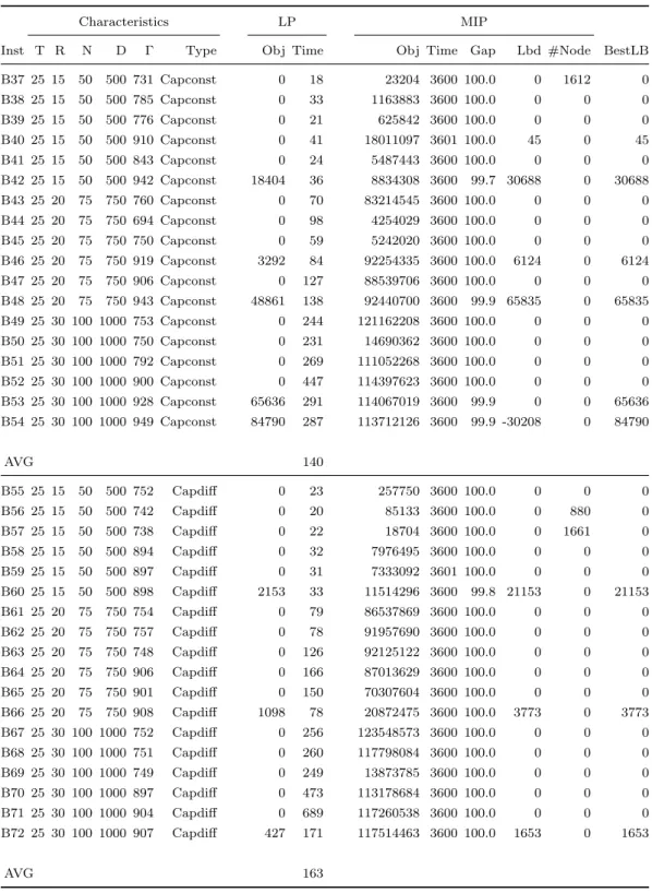
2.5.2 MIP Formulation Comparison without Considering Setup Cost . . 52

2.6 Conclusions . . . 62

3 Complex Capacitated Lot Sizing Problem: Heuristics 63 3.1 Introduction . . . 64

3.2 Constructive Heuristic Algorithms . . . 64

3.2.1 Fix&Relax Algorithm . . . 64

3.2.2 Product Decomposition Based Algorithm . . . 67

3.2.3 First Solution Heuristic Algorithm Based on LP Relaxation . . . . 75

3.3 Fix&Optimize algorithm . . . 81

3.4 Computational Results . . . 81

3.4.1 Algorithm Parameter Evaluation . . . 82

3.4.2 Algorithm Comparison Results . . . 86

3.5 Conclusions . . . 99

4 Production Planning Solution to the Apparel Application 100 4.1 Decomposition Approach . . . 101

4.2 Application Performance Analysis . . . 105

4.3 Conclusions . . . 106

5 Capacitated Lot Sizing Problem with A Fixed Product Sequence 107 5.1 Capacitated Lot Sizing Problem with Sequence Dependent Setup . . . 108

5.2 Problem Definition . . . 110

5.3 Problem Formulation . . . 116

5.4 A Special Case Study . . . 122

5.5 Column Generation Approach . . . 127

5.6 Computational Results . . . 130

5.7 Conclusions . . . 133

6 General Conclusion and Future Work 134 Appendix A Data Analysis and Computational Results 137 A.1 CLSC Computational Results . . . 139

A.2 CLSP-FS1 Computational Results . . . 149

1.1 Production planning example: demands . . . 2

1.2 Production planning example: minimum manufacturing cost solution . . . 3

1.3 Production planning example: minimum inventory cost solution . . . 3

1.4 Production planning example: minimum overall cost solution . . . 3

1.5 Overview of review papers of deterministic dynamic LSP . . . 7

1.6 Apparel manufacturing production: learning curve example . . . 15

1.7 Modeling apparel production planning to lot sizing problem . . . 16

2.1 CLSC Example 2.1 data: setups . . . 21

2.2 CLSC Example 2.1 data: capacities . . . 21

2.3 CLSC formulation size comparison . . . 32

2.4 CLSC benchmark instances summary . . . 35

2.5 CLSC real-world benchmark instances . . . 36

2.6 CLSC pseudo-randomly generated benchmark instances . . . 43

2.7 CLSC instance generator parameters . . . 43

2.8 CLSC formulation comparison with setup cost . . . 51

2.9 CLSC formulation comparison without setup cost . . . 53

2.10 CLSC feature - complexity analysis . . . 55

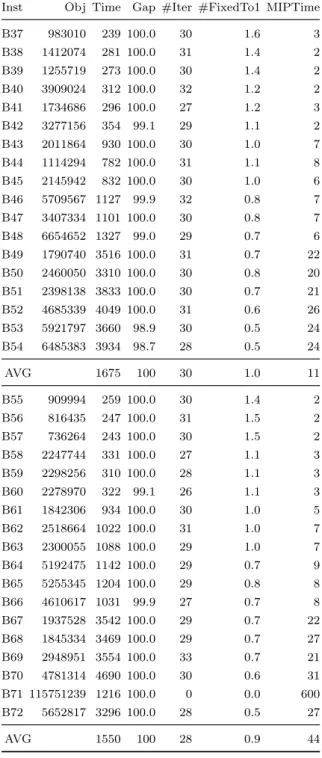
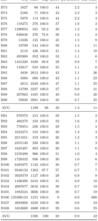
2.11 Computational results: CPLEX on IAP-B . . . 56

2.12 Computational results: CPLEX on IRG-B (1) . . . 57

2.13 Computational results: CPLEX on IRG-B (2) . . . 58

2.14 Computational results: CPLEX on IRG-B (3) . . . 59

3.1 PD algorithm: sorting criteria . . . 68

3.2 PD algorithm: sub-problem . . . 69

3.3 Comparison results: F&R algorithm variations . . . 83

3.4 Comparison results of PD algorithm variations: sub-problems . . . 84

3.5 Comparison results of PD algorithm variations: sorting criteria . . . 85

3.8 Computational results: FSH algorithm on IRG-B (2) . . . 89

3.9 Computational results: FSH algorithm on IRG-B (3) . . . 90

3.10 Computational results: heuristic algorithm on IAP-B . . . 92

3.11 Computational results: heuristic algorithm on IRG-B summary . . . 93

3.12 Computational results: heuristic algorithm on IRG-B summary by type . 94 3.13 Computational results: heuristic algorithm on IRG-B (1) . . . 96

3.14 Computational results: heuristic algorithm on IRG-B (2) . . . 97

3.15 Computational results: heuristic algorithm on IRG-B (3) . . . 98

4.1 Detailed and aggregated model in planning phase . . . 103

4.2 Application planning solution evaluation . . . 106

5.1 CLSP-FS1 Example 5.1 data . . . 113

5.2 Theorem 5.2 proof CLSP-FS1-LT instance parameters . . . 123

5.3 Computational results: CLSP-FS1 formulation comparison . . . 130

5.4 Computational results: column generation heuristic based on AG-SO . . . 131

5.5 Computational results: CLSP-FS1-LT formulation comparison . . . 132

1.1 DecisionBrain production planning applications . . . 4

1.2 Technical structure of lot sizing problem in Glock et al. [55] . . . 6

1.3 Apparel manufacturing application: plant structure . . . 13

1.4 Apparel manufacturing application: production procedure . . . 14

2.1 Setup carryover . . . 20

2.2 Time window of demand . . . 20

2.3 CLSC Example 2.1 data: time windows . . . 21

2.4 CLSC Example 2.1 optimal solution with setup cost . . . 22

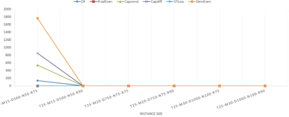
2.5 CLSC instance R5 analysis: machine capacity distribution . . . 37

2.6 CLSC instance R5 analysis: production time distribution . . . 38

2.7 CLSC instance R5 analysis: setup time distribution . . . 38

2.8 CLSC instance R5 analysis: product-demand distribution . . . 39

2.9 CLSC instance R5 analysis: demand quantity distribution . . . 39

2.10 CLSC instance R5 analysis: demand time window distribution . . . 40

2.11 CLSC instance R5 analysis: demand release/due date distribution . . . . 41

2.12 CLSC instance R5 analysis: capacity requirement by time interval . . . . 42

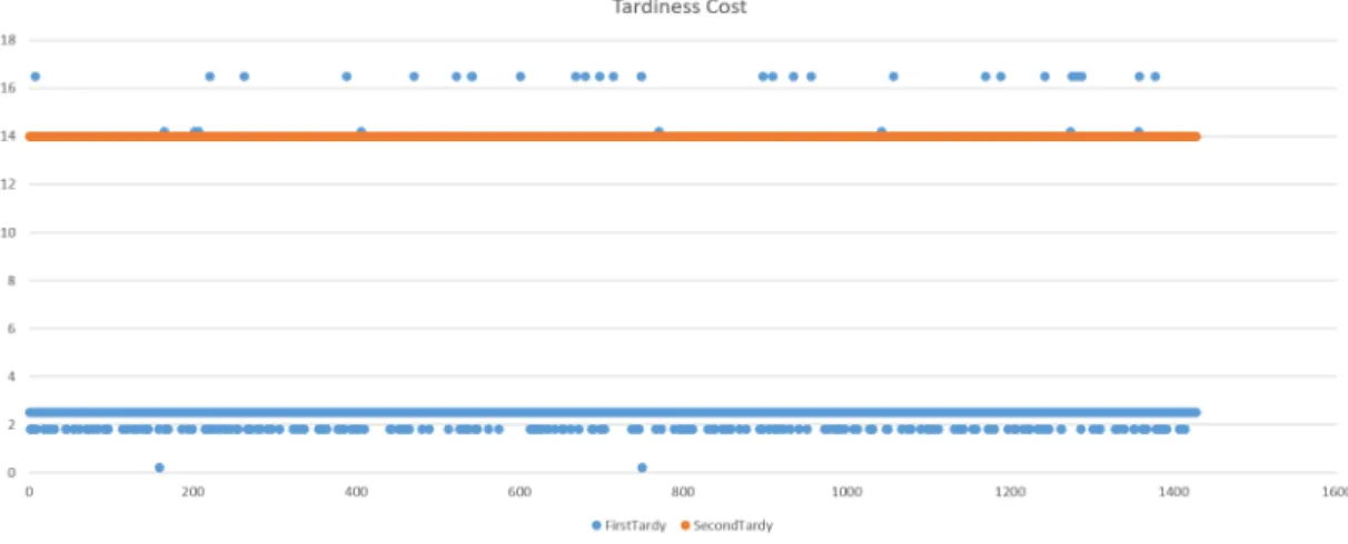
2.13 CLSC instance R5 analysis: tardiness cost distribution . . . 42

2.14 LPR time on different types of instances . . . 60

2.15 MIP gap on different types of instances . . . 61

2.16 MIP number of nodes on different types of instances . . . 61

3.1 FR-T algorithm procedure Absi and Kedad-Sidhoum [3] (modified) . . . . 66

3.2 PD algorithm flow chart . . . 68

3.3 PD-SI algorithm capacity update example . . . 73

3.4 FSH algorithm flow chart . . . 76

3.5 CLSC Example 2.1 optimal solution (no setup cost) . . . 77

3.6 CLSC Example 2.1 optimal LP relaxation solution (no setup cost) . . . . 77

3.9 Heuristic algorithm comparison results on pilot instances . . . 93

4.1 Apparel manufacturing decomposition approach . . . 101

5.1 Color change in production . . . 111

5.2 Definition 5.1 illustration . . . 112

5.3 CLSP with sequence dependent setup Example 5.1 optimal solution . . . 113

5.4 CLSP-FS1 Example 5.1 optimal solution . . . 113

5.5 Theorem 5.1 CLSP-FS1 instance optimal solution structure . . . 114

5.6 CLSP-FS1 graph representation of setup sequence . . . 119

5.7 Theorem 5.2 reduction from CLSP with single product to CLSP-FS1-LT . 123 5.8 CLSP-FS1 network representation of the pricing problem . . . 128

Industrial and Scientific Context

In this manuscript, our research focuses on production planning. The problem is to optimize production plan in manufacturing industry to achieve high customer service level and cost efficiency. Due to our industrial background, we have been exposed to various types of world applications. Therefore, all our research is motivated by real-istic requirements that we have encountered in building industrial production planning solutions. First, we have studied a production planning problem from apparel manu-facturing industry. This problem is brought to our attention by a project that we have worked with a market leader in the apparel industry, which produces 60% of the T-shirts sold in the US. Our research result, including modeling and algorithm design, has been implemented inside the engine of their production planning and scheduling software and improves the daily production efficiency. Second, we have studied a restricted version of a classical production planning problem: capacitated lot sizing problem with sequence dependent setups, which is known to be hard to solve. This newly proposed model con-siders the planners knowledge in certain industries and therefore simplifies the classical model. By doing so, there is a better chance to deliver reasonable production planning solutions for industries where our model is applicable.

This chapter is organized as follows: In Section 1.1, we present our research back-ground and introduce our study interest at production planning. In Section 1.2, we describe a general picture of production planning, i.e., lot sizing problem. In Section 1.3, the real-world application of production planning problem in apparel manufacturing is introduced. Finally, we summarize major contributions of our research in Section 1.4 as a reading guide for the rest of this manuscript.

1.1

Introduction

Our research is performed under the CIFRE program (Conventions Industrielles de For-mation par la REcherche) [30]. Therefore, it is a collaboration between Paris Dauphine University and DecisionBrain (https://www.decisionbrain.com). DecisionBrain is a soft-ware company that delivers advanced analytics and optimization solutions to innovative companies who want to apply a scientific approach to decision making. Building pro-duction planning and scheduling solution is one of DecisionBrain’s expertise.

Generally speaking, production planning is to decide the production for a future period of time (planning horizon) given limited resources and/or production restrictions to achieve optimal customer service level and cost efficiency. Here is a small example modified from [108] to illustrate the concept. An apparel manufacturer produces different types of costumes. One specific type of costumes requires a high setup cost due to the special technique and equipment needs, therefore at most one batch can be produced in one month. Given 200 units of stock at the end of the year, the goal is to plan the production of this costume for the next 8 months (January to August) to minimize the cost while satisfy all forecasted demands. The cost includes: setup cost as $5000 if there is a positive production in a month, unitary processing cost $100, and unitary inventory cost $5. The demand forecast for the next 8 months is given in Table 1.1 and we need to decide the production quantity for each month.

Table 1.1: Production planning example: demands

Jan Feb Mar Apr May Jun Jul Aug 400 400 800 800 1200 1200 1200 1200

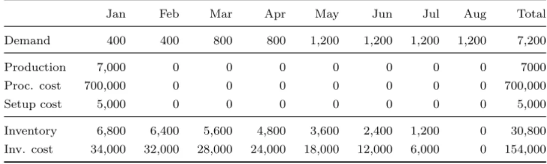
If it is only to minimize the manufacturing cost (setup cost and production cost), we can produce only once in January to satisfy total demands till August. The solution is given in Table 1.2 and the total cost equals to $859,000. This cost includes $700,000 (7,000 x 100) processing cost, $154,000 (30,800 x 5) inventory cost and $5,000 (5,000 x 1) setup cost. If it is only to minimize the inventory cost, we can follow the just-in-time rule and produce in each month the amount it requires. The total cost becomes $740,000 and the solution is given in Table 1.3. However, if it is to minimize the overall cost, the optimal solution has total cost equals to $736,000 and the optimal solution is given in Table 1.4. In the optimal solution, there are two months (February and April) that have no production.

Table 1.2: Production planning example: minimum manufacturing cost solution

Jan Feb Mar Apr May Jun Jul Aug Total Demand 400 400 800 800 1,200 1,200 1,200 1,200 7,200 Production 7,000 0 0 0 0 0 0 0 7000 Proc. cost 700,000 0 0 0 0 0 0 0 700,000 Setup cost 5,000 0 0 0 0 0 0 0 5,000 Inventory 6,800 6,400 5,600 4,800 3,600 2,400 1,200 0 30,800 Inv. cost 34,000 32,000 28,000 24,000 18,000 12,000 6,000 0 154,000 *Initial inventory = 200

Table 1.3: Production planning example: minimum inventory cost solution

Jan Feb Mar Apr May Jun Jul Aug Total Demand 400 400 800 800 1,200 1,200 1,200 1,200 7,200 Production 200 400 800 800 1,200 1,200 1,200 1,200 7000 Proc. cost 2,000 4,000 8,000 8,000 12,000 12,000 12,000 12,000 700,000 Setup cost 5,000 5,000 5,000 5,000 5,000 5,000 5,000 5,000 40,000 Inventory 0 0 0 0 0 0 0 0 0 Inv. cost 0 0 0 0 0 0 0 0 0 *Initial inventory = 200

Table 1.4: Production planning example: minimum overall cost solution

Jan Feb Mar Apr May Jun Jul Aug Total Demand 400 400 800 800 1,200 1,200 1,200 1,200 7,200 Production 600 0 1,600 0 1,200 1,200 1,200 1,200 7,000 Proc. cost 60,000 0 160,000 0 120,000 120,000 120,000 120,000 700,000 Setup cost 5,000 0 5,000 0 5,000 5,000 5,000 5,000 30,000 Inventory 400 0 800 0 0 0 0 0 1,200 Inv. cost 2,000 0 4,000 0 0 0 0 0 6,000 *Initial inventory = 200

Even in this toy example, we can have an insight of the benefit that production planning may bring to the industry. Kellogg Company reports annual cost savings of 4 million dollars by performing optimization to plan the production and distribution decisions for its cereal and convenience foods business [108]. Thanks to the development of IT technology and commercial optimization software, it becomes possible to tackle large scale real-world production planning problems using optimization. Therefore, more and more companies start to realize that introducing scientific method to optimize the

decision process could have a non-negligible impact on their profits and competences. Another reason of the tremendous interest shown in literature in production planning is that different manufacturing industry implies different production planning problems. Therefore production planning problems occur with many variations each with its own complexity and challenges. For instance, to the best of our knowledge, production planning problems studied in this manuscript have never been addressed before.

There are several production planning projects explored in DecisionBrain from dif-ferent industries, such as apparel manufacturing, semi conductor assembling and test-ing, and disposable table-ware production (Figure 1.1). Research presented in this manuscript is mainly motivated by the project with an apparel company, which is to build a production planning and scheduling software to arrange mid term and short term productions. The details of this application is presented in Section 1.3. But first of all, we give a general introduction on the production planning problem in Section 1.2, which is also referred as lot sizing problem.

Figure 1.1: DecisionBrain production planning applications

1.2

Production Planning: Lot Sizing Problem

Lot sizing problem

Lot Sizing Problem (LSP) is to plan production resources and activities, especially de-termine production quantities, to achieve the economical cost and/or more intangible

objectives such as customer service level. The history of LSP can be traced back to the publication of Harris [71], which proposes the Economic Order Quantity (EOQ) model. This problem has continuous time model with infinite time horizon, and all parame-ters such as demand quantity and inventory holding cost are constant. The solution of this problem can be obtained by a formula directly. Later, different extensions of EOQ have been studied such as Economic Lot Scheduling Problem (ELSP), which extends the problem to multi-item and considers capacity constraints. It is shown to be NP-hard in Gallego and Shaw [52]. However, both EOQ and ELSP consider constant parameters, which is not always the case in real applications. The Wagner-Whitin (WW) model was studied in the seminal papers of Wagner and Whitin [131] and Manne [96] in late 50’s. In this model, the planning horizon is decomposed into time buckets and demand quan-tities vary with time buckets. Therefore, the WW model extends constant parameters to dynamic parameters varying with time and thus is referred to dynamic LSP.

The WW model is defined as follows: Given a planning horizon with T time buckets, let dt be the product demand quantity for each time bucket t∈ {1, 2, . . . , T }. The unit

inventory holding cost is ht. Moreover, in each time bucket, to produce a positive

quan-tity of products, there is a setup cost sct. The problem is to determine the production

quantity in each time bucket so that all demands are satisfied with minimum cost. This problem can be formulated as follows:

min T X t=1 htIt+ sctzt s.t. I_t−1+ xt= dt+ It t∈ {1, 2, . . . , T } I0 = IT = 0 xt≤ btzt t∈ {1, 2, . . . , T } x∈ RT+, I ∈ RT +1+ , z ∈ {0, 1}T (1.1)

where bt is the maximum production quantity in time bucket t.

Different classification schemes are used in literature reviews of LSP such as De Bodt et al. [33], Drexl and Kimms [40], Staggemeier and Clark [123] and Guner Goren et al. [64]. One of the classification scheme divide LSP from two dimensions: models with stationary or dynamic parameters, models with deterministic or stochastic parameters (see Figure 1.2). According to this classification scheme, the EOQ and ELSP will lie in the stationary model whereas the WW model and its extensions lie in the dynamic model.

Figure 1.2: Technical structure of lot sizing problem in Glock et al. [55]

In this manuscript, our focus is the deterministic extensions of the WW model, which is Deterministic Dynamic LSP with finite time horizon (DDLS). Giving a comprehensive survey on the literature of DDLS becomes an “impossible mission” due to the flourish research in this domain. For more than half a century development of DDLS, more than 30 literature review papers and books have been published and even two reviews of literature reviews on production planning and inventory management are given by Glock et al. [55] and Guiffrida et al. [62]. To avoid duplication but still provide a set of references for interested readers, we summarize the survey papers related to DDLS in Table 1.5. They are from Glock et al. [55] and Guiffrida et al. [62] together with several papers and books that we believe worth mentioning.

Some papers are not included in the table since their focus is not lot sizing problem. For example, Gelders [53] mainly focuses on the state of the art progress in the production planning, where LSP takes only one section. It covers the WW model, multi-level uncapacitated LSP, capacitated LSP and ELSP, mainly from the perspective of heuristic algorithms. Bitran and Yanasse [17] studies the capacitated LSP and gives complexity analysis over various cost structures. Nahmias [101] gives an overview of the perishable ordering policy, only one paper about deterministic LSP is mentioned, which has random decay.

1. INDUSTRIAL AND SCIENTIFIC CONTEXT 7

Reference Content Classification

Aggarwal [5] General view of inventory models. Dynamic/static model, number of items, number of loca-tions and echelons, characteristics of demand, research ob-jective.

De Bodt et al. [33] Dynamic LSP with constant costs over time. Fixed/rolling horizon, deterministic/probabilistic model, single/ multi level.

Bahl et al. [13] General review from both practitioner and research based literature.

Single/multi level, unconstrained/constrained resources. Aksoy and Selcuk Erenguc [7] Multi-item single stage inventory systems with joint setup

costs.

Deterministic (static/dynamic models) and stochastic (con-tinuous review/periodic review).

Maes and Wassenhove [95] Classification and computational review on heuristic algo-rithms of the multi-item single-level capacitated LSP.

Single-resource heuristics (special-purpose methods), and mathematical-programming-based heuristics (general). Zoller and Robrade [137] A review and experimental comparison of algorithms of the

WW model with rolling horizon.

Gupta and Keung [66] Multi-stage lot-sizing. Constant/dynamic demands, rolling horizon. Raafat [111] Mathematical modelling of deteriorating inventory system

especially deterioration as a function of the on-hand level of inventory.

Deteriorating features, LSP features.

Kuik et al. [91] General view on models. Strategic/tactical/operational, modeling elements in the LSP (such as planning horizon, static/dynamic demands). Wolsey [132] Single item uncapacitated LSP.

Benton and Park [16] LSP with several types of discount schemes. Four discount types are surveyed from both the buyer point of view and the supplyer point of view.

Drexl and Kimms [40] General review of the LSP and scheduling. Single/multi level. For the single level, discrete time and continuous time model are considered.

Goyal and Giri [61] The deteriorating inventory literature review as a continua-tion of Raafat [111].

Shelf life, demand variations and other conditions or con-straints.

Rizk and Martel [113] Material flow planning in a supply chain, and in particular with deterministic lot-sizing methods.

Single/multiple facility, single/multiple level, single/ mul-tiple items, capacitated/uncapacitated, deterministic/ stochastic, static/dynamic demand.

1. INDUSTRIAL AND SCIENTIFIC CONTEXT 8

Reference Content Classification

Staggemeier and Clark [123] LSP and scheduling models and its algorithms. Time period, multi machines and other constraints. Karimi et al. [88] Models and algorithms of capacitated LSP with single level. Planning horizon, number of levels, number of

prod-ucts, capacity or resource constraints, deterioration items, static/dynamic/deterministic/stochastic demand, setup structure, inventory shortage.

Brahimi et al. [22] Single item LSP. Big/small time buckets, uncapacitated (extensions such as backlogging, multiple facilities) and capacitated (different cost structures).

Pochet and Wolsey [108] Mixed integer programming formulations for the LSP and its variants

Zhu and Wilhelm [136] LSP and scheduling with sequence dependent setup.

Jans and Degraeve [84] An overview of the use of meta-heuristics for solving LSP. Algorithm representation, evaluation, neighborhood defini-tion and genetic operators.

Jans and Degraeve [85] Modeling deterministic single-level dynamic LSP based on various industrial extensions.

Basic LSP models and their extensions from two directions: modeling the operational aspects in more details, or is more towards tactical and strategic models.

Quadt and Kuhn [109] Extensions of the capacitated LSP: back-orders, setup carry-over, sequencing, and parallel machines.

Back-orders, setup carry-over, sequencing, and parallel ma-chines.

Allahverdi et al. [8] LSP with setup cost and setup times.

Robinson et al. [114] Updates the review by Aksoy and Selcuk Erenguc [7] of the coordinated LSP.

Single/multiple items, coordinated/uncoordinated setup cost structures, capacitated/uncapacitated.

Buschk¨uhl et al. [25] Mainly survey the algorithms for the dynamic capacitated LSP for single level and multi level.

Mathematical programming heuristics, Lagrangian heuris-tics, decomposition and aggregation heurisheuris-tics, metaheuris-tics, problem-specific greedy heuristics.

Guner Goren et al. [64] A review of applications of genetic algorithms in LSP. Static/dynamic, single/multi level, capaci-tated/uncapacitated

Capacitated Lot sizing problem

Among all problems in the domain of DDLS, our focus is at one type of LSP which considers the limited resource/machine capacity, called Capacitated Lot Sizing Problem (CLSP). Considering different features and cost structures will lead to different types of CLSP. Based on problems studied in this manuscript, we introduce the CLSP model with following parameters:

• N = {1, 2, . . . , N} a set of N products. • T = {1, 2, . . . , T } a set of T time periods.

• capt: machine capacity in each time period t∈ T .

• dit: demand of each product i∈ N in time period t ∈ T .

• pti: unitary production time of each product i∈ N .

• hcit: unitary inventory cost of each product i∈ N in time period t ∈ T .

• bit: maximum amount of production i that can be produced in t∈ T .

• sti: setup time to product i∈ N .

• sci: setup cost to product i∈ N .

CLSP is to decide the production quantity of each product in each time bucket so that all demands are satisfied with a minimum total cost while respecting machine capacities. Due to the capacity constraints, the problem is shown to be NP-hard even when there is only a single product by Florian et al. [47] and Bitran and Yanasse [17]. In the case of multiple products, Chen and Thizy [28] proved that it is strongly NP-hard. Karimi et al. [88] have done a nice survey focusing on CLSP with production cost and its solution approaches. Quadt and Kuhn [109] have provided a survey of CLSP with extensions including back-orders, setup carryover, sequencing and parallel machine.

Developing mathematical formulations is the very first step of our research since problems studied in this manuscript have not been studied before to the best of our knowledge. Therefore, in this section, we recall three Mixed Integer Programming (MIP) formulations of CLSP that have been studied and often adapted to other extensions of CLSP in the literature. These formulations are aggregated formulation, facility location formulation and network formulation.

Aggregated (AG) formulation is an intuitive formulation and was proposed by Trigeiro et al. [129]. We introduce following variables for each product i∈ N and time bucket t_{∈ T :}

• xit∈ R+: quantity of product i produced in time bucket t;

• Iit∈ R+: inventory of product i at the end of time bucket t;

• zit∈ {0, 1}: it equals to 1 if product i is produced in time bucket t, 0 otherwise.

The formulation is given as follows:

min X i∈N ,t∈T hcitIit+ X i∈N ,t∈T scizit (1.2) s.t. Ii,t−1+ xit= Iit+ dit i∈ N , t ∈ T (1.3) X i∈N ptixit+ X i∈N scizit≤ capt t∈ T (1.4) xit≤ bitzit i∈ N , t ∈ T (1.5) xit, Iit≥ 0, Ii,0 = 0 i∈ N , t ∈ T (1.6) zit∈ {0, 1} i∈ N , t ∈ T (1.7)

The objective function (1.2) is to minimize the total cost including inventory cost P

i∈N ,t∈T hcitIit and setup cost P_{i∈N ,t∈T} scizit. Constraints (1.3) ensure material

bal-ance for each product i in each time bucket t that the total inflow (last bucket ending inventory and production quantity) equals to the outflow (demand dit and ending

in-ventory). Constraints (1.4) guarantee the capacity usage does not exceed the available capacity in each time bucket. Finally, constraints (1.5) link production with setup: there is only a production if there is a corresponding setup for each product in each time bucket.

Facility Location (FL) formulation was first proposed by Krarup and Bilde [90] for cases without capacity restrictions. It is also referred as the transportation problem formulation [34] and simple plant location formulation [90]. Later it has been adapted to other LSP [124]. We introduce decision variables as follows for each product i∈ N , time bucket t, k such that t_{≤ k ∈ T :}

• xitk ∈ R+: quantity of product i produced in time bucket t to satisfy demand in

later time bucket k;

• zit ∈ {0, 1} is defined as before, it equals to 1 if product i is produced in time

The formulation is given as follows: min X i∈N ,t∈T hcit   X s∈T :s≤t X k∈T :t<k xisk   + X i∈N ,t∈T scizit (1.8) s.t. X k∈T :k≤t xikt= dik i∈ N , t ∈ T (1.9) X i∈N pti   X k∈T :t≤k xitk   + X i∈N ,t∈T stizit≤ capt t∈ T (1.10) xitk≤ min{bit, dik}zit i∈ N , t ∈ T , t ≤ k ∈ T (1.11) xitk≥ 0 i∈ N , t ∈ T (1.12) zit ∈ {0, 1} i∈ N , t ∈ T (1.13)

There is a direct link between variables introduced in AG model and those introduced in FL formulation: xit= X k∈T :t≤k xitk Iit= X s∈T :s≤t X k∈T :t<k xisk

Therefore, the objective function is a simple substitution. Constraints (1.9) state that the total production quantity dedicated for demand dik equals to the demand quantity.

Constraints (1.11) link the production quantity xitk with the corresponding setup zit.

Here the upper bound of xitk is no greater than the upper bound of xit, which is the

main reason that FL is stronger than AG formulation in the sense of better lower bound from Linear Programming (LP) relaxation. The price for the tighter lower bound is the number of variables, which is increased to O(N T2).

Network (NW) formulation was first proposed by Eppen and Martin [42]. It is also referred as shortest path/route formulation [34, 122]. We introduce decision variables as follows for each product i_{∈ N , time bucket t, k such that t ≤ k ∈ T :}

• uitk∈ [0, 1]: fraction of total demand from time bucket t through k of item i that

is produced in t;

• zit ∈ {0, 1} is defined as before, it equals to 1 if product i is produced in time

bucket t, 0 otherwise.

We also define following constant for simplicity of the formulation:

Ditk= k X v=t div, Hitk= k X v=t+1

h_i,v−1Divk, IDitk =

(

1 if Ditk> 0

The formulation is given as follows: min X i∈N ,t∈T ,k∈T :k≥t Hitkuitk+ X i∈N ,t∈T scizit (1.14) s.t. X i∈N ,k∈T :k≥t ptiDitkuitk+ X i∈N ,t∈T stizit≤ capt t∈ T (1.15) X t∈T ui1t = 1 i∈ N (1.16) X k∈T :k≤t−1 u_i,k,t−1 = X k∈T :k≥t uitk i∈ N , 1 < t ∈ T (1.17) X k∈T :k≤t IDitkuitk≤ zit i∈ N , t ∈ T (1.18) uitk≥ 0 i∈ N , t ∈ T (1.19) zit ∈ {0, 1} i∈ N , t ∈ T (1.20)

The formulation is easier to understand if we see variables uitk only as binary value.

Then based on the proof in [42], the formulation is still valid when uitk ∈ [0, 1]. When

u_itk= 1, its corresponding production quantity equals to D_itk and inventory cost equals to Hitk. The objective function (1.14) is still to minimize the inventory cost and setup

cost. Constraints (1.15) ensure capacity restriction in time bucket t. Constraints (1.16) and (1.17) represent flow balance constraints for the source node and other nodes in the underlying network. Constraints (1.18) link production with its corresponding setup for each product i in time bucket t.

FL and NW models are stronger reformulation of AG model for CLSP. Nemhauser and Wosley [104] has shown that in the uncapacitated case, both LP relaxations of FL and NW define the convex hull of the problem. Denizel et al. [34] further proved the equivalence of the LP relaxations of FL and NW formulations for CLSP with constant unitary inventory cost hi. They also point out that FL formulation has more constraints

while its constraint matrix is less dense and has smaller coefficients, therefore different characteristics may be exploited to choose between these two reformulations.

In the next section, we start from another perspective and introduce the real-word application that motivates the first part of our research.

1.3

Production Planning in An Apparel Manufacturing

Application

The main problem studied in this manuscript is brought to our attention by a project in manufacturing industry. The company is a market leader in the apparel industry,

which produces 60% of the T-shirts sold in the US. On-time delivery, low production and shipping cost is a critical competitive advantage for the company. To achieve this goal on such large scale, it is essential to optimize production planning and scheduling to perform efficient production. To model and solve the underlying production planning problem, we need to first understand the manufacturing procedure and bottlenecks in this particular case study. Hence, in Section 1.3.1, we first present the apparel company, its manufacturing procedure and bottlenecks. In section 1.3.2, we present the modeling of the problem, which leads to the CLSP studied in Chapters 2 - 4.

1.3.1 An Apparel Manufacturing Application

The company has 10 manufacturing plants over Asia, however, they are independent on the production planning and scheduling level. Therefore, the problem scope is considered as a single plant. A plant layout example is shown in Figure 1.3. In each plant, there are several work centers, each of which corresponds to a production operation. In other words, to produce one piece of clothes, it has to go through several work centers to finish. Moreover, there are normally more than one machine in each work center. Therefore, the production planning has to decide the production quantity for each production line. This implies parallel machines in the underlying lot sizing problem and leads to the first difficulty of the problem.

Figure 1.3: Apparel manufacturing application: plant structure

To produce one piece of clothes, all or some of following operations have to be done in sequence which includes cutting, embroidery, sewing, washing, ironing/dipping, packing and cartoning. In Figure 1.4, we show the entire manufacturing processes. Each product has a specific production routing. Some orders will route through all the operations, while some orders may skip certain operations (such as washing). On the other hand, some orders will go through the ironing operation, while some orders will go through dipping operation instead. Among all these processes, we could identify a bottleneck

step, which is the sewing process. This is not only because that it mainly depends on workers instead of machines but also because that it consumes most of the time during the production cycle. Due to this reason, we only model the production planning on the sewing process, which leads to the lot sizing problem with single level. Sewing process is the craft of fastening or attaching objects using stitches made with a needle and thread. There are about 20 to 60 sewing lines in each plant. Each sewing line is a group of sewing workers who share the same working shift schedule. Different sewing lines may have different number of workers and different working hours per day, which results in different machine capacities in the lot sizing problem. This together with multiple productions lines leads to the second difficulty because all parallel machines are not identical.

Figure 1.4: Apparel manufacturing application: production procedure

As an apparel company, it produces different types of products such as T-shirts, pants and costumes. In fact, each client demand corresponds to one particular product. This is the third difficulty of our problem that 400 to 1000 products have to be produced in the realistic instances. Different products have different unitary processing time therefore can not be aggregated directly.

Products can be grouped into about 400 different styles in total, which can be further grouped into about 50 style families (currently they are regrouping them to 150+ style families). On a sewing line, changing the style family from one to another requires a setup and an efficiency loss, which is known as learning curve. In this application, the learning curve is given as a list of worker efficiency over 10 working days instead of a function (see example in Table 1.6). Given a product, the processing time of sewing is given by the time needed to process one item divided by the efficiency of the sewing line (which is 1 maximum). To achieve the best efficiency, the same style family is usually

kept for a few days (1 to 2 style families per week) on a sewing line. For small orders, style family can be changed daily. Within the same style family, a style change will also cause a setup cost and setup time, which is minor comparing to style family change. This leads to the fourth difficulty of our problem that setup is sequence dependent, i.e., it depends not only on the current product but also the previous product. LSP with sequence dependent setup is known to be very hard to solve since there is Traveling Salesman Problem embedded inside.

Table 1.6: Apparel manufacturing production: learning curve example

Day Day1 Day2 Day3 Day4 Day5 Day6 Day7 Day8 Day9 Day10 Efficiency 0.6 0.65 0.7 0.8 0.9 1.0 1.0 1.0 1.0 1.0

Each sales order, i.e., demand, specifies the product required, the quantity, the ship-ping destination and the due date. It is allowed to delay the delivery or even cancel the delivery of a sale order, however, corresponding penalty will be charged accordingly. There are two levels of tardiness cost. The first level corresponds to a shipment cost by airplane instead of maritime to catch up the due date. The second level corresponds to a compensation for the orders delivered too late. This leads to a different model from classical LSP that we have introduced in Section 1.2 that demands can be delayed or lost with penalty cost, and the cost is defined during a interval. This feature is often referred as lost sale and backlogging in the literature.

Some aspects are out of the scope of this project. First, the ordering and management of raw material. The existing MRP system will generate the earliest available date for all the raw materials in an order. This date will be used as the earliest possible start time for an order. Second, demand forecasting. All work orders confirmed or forecasted are treated the same as an input to our system. However, as one way to reduce uncertainty, forcasted demands also have a start date to prevent them from producing too early. Therefore, we have a release date for each demand that only after which the production for this demand can start.

To make use of the planning resources efficiently, the company would like to plan its production activities for a future period of time, which is called planning horizon. The duration of the planning horizon considered is between 24 weeks to 56 weeks. The major objective of the production planning includes: maximization of the on-time delivery rate, minimization of the late shipment cost (including expediting transportation cost and sales loss cost), minimization of the learning curve loss and setup costs on the sewing lines. The minimization of the labor cost (due to overtime) is also one goal which is not

considered in the project currently.

1.3.2 Production Planning Problem Modeling

To be able to optimize the production planning in this apparel project, we first have to extract the mathematical model out of the context. Modeling large scale real-world application is always a trade-off between accuracy and solvability, and often has a big impact on the solution quality. In Table 1.7, we present the mapping between the application aspects presented in previous section to a lot sizing problem we will study in following chapters.

Table 1.7: Modeling apparel production planning to lot sizing problem

Application Lot sizing Problem Planning horizon 20 - 30 weeks Weekly time buckets

7 production process step Bottleneck sewing process, single level LSP Multiple sewing production lines Non-identical parallel machines

300 - 1000 products, 1 - 80 style families Aggregated product for each style family Sequence dependent learning curve Setup carryover

Demand release date Production time window Demand can be lost or delayed Lost sales and backlogging

Lot sizing problem with up to seven levels is very complex. Therefore, we only model the bottleneck process and study the single level LSP. Modeling setup and learning curve accurately on the sewing production line will dramatically increase the problem complexity. In order to achieve reasonable performance, we simplify the problem in the production planning level and deal with them in the scheduling phase. First, all setup between styles within the same style family is ignored. Second, each learning curve is transformed to a total capacity loss. In our example in Table 1.6, the efficiency loss equals to (1_{− 0.6) + (1 − 0.65) + (1 − 0.7) + (1 − 0.8) + (1 − 0.9) = 1.35. Then the} capacity loss will be 1.35_{× dailyCapacity and the new setup time equals to capacity} loss, which depends on both products and production lines. Third, we relax the sequence dependent setup to setup carryover so that the model still prefers to keep the same style family on a production line, but with less complexity.

In summary, the lot sizing problem based on this project consists of single level production, multiple products, parallel machines, backlogging, lost sale, production time window and setup carryover. To the best of our knowledge, this problem is first studied in this manuscript. We will formally define the problem and perform study on it in the following chapters. In the next section, we summarize our major contributions.

1.4

Contributions

In this section, we provide a contribution summary of our research, which can be used as a reading guide for the rest of this manuscript.

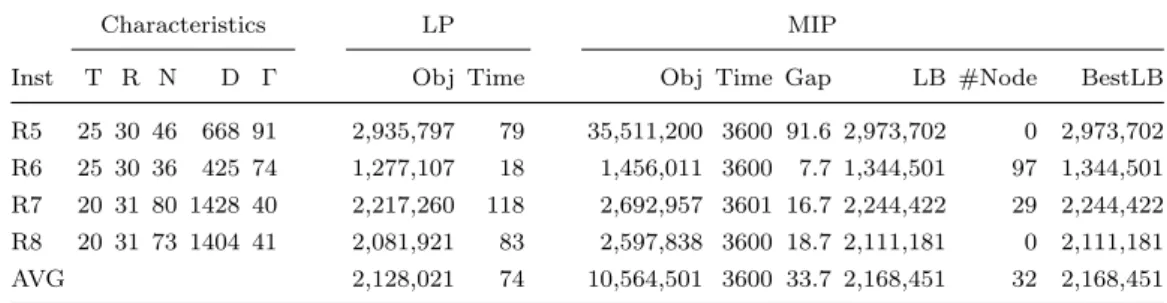
First of all, a complex capacitated lot sizing problem with setup carryover is formu-lated and studied, which is based on the real-world application introduced in Section 1.3. The problem is shown to be NP-hard and different MIP formulations are proposed in Chapter 2. Two sets of benchmark instances are presented to evaluate these formu-lations. One set consists of real-world application instances, whereas the other set is pseudo-randomly generated and simulates characteristics observed from real-world in-stances. The computational results show that the problem can not be solved within rea-sonable time limit by the standard MIP solver CPLEX. Therefore, heuristic algorithms are developed to tackle this problem in Chapter 3. Both constructive and improving heuristic algorithms are developed. We perform experimental tests to evaluate perfor-mances of all developed heuristic algorithms and show the efficiency of our algorithms compared to the standard MIP solver CPLEX. In Chapter 4, our study results are im-plemented in the production planning engine for the apparel company and we show the complete industrial production planning solution.

Second, a special case of capacitated lot sizing problem with sequence dependent setup is studied in Chapter 5, which is called CLSP with a fixed product sequence. In many manufacturing industry, switching production from one product to another will cause setup operations. The setup will consume limited machine capacity and/or cause a setup cost. When the setup depends on the production sequence, i.e., the setup to produce current product depends on both itself and the previous produced product, it is called sequence dependent setup [46, 63]. In this case, both lot sizing and sequencing decisions have to be made. The difficulty of this problem lies in the factorial number of setup sequence candidates to be chosen from for each time bucket. However, in certain manufacturing industries, this number may be reduced if we restrict the model based on the planners’ knowledge. We consider a restricted model in which the number of potential setup sequences is reduced to O(n2n) compared to O(n!) for the CLSP with sequence dependent setups. The problem is shown to be NP-hard, and a column generation heuristic is developed. A set of benchmark instances is tested and computational results are presented to evaluate the algorithm performance.

Complex Capacitated Lot Sizing

Problem: Formulations and

Benchmarks

A complex capacitated lot sizing problem is constructed from the apparel manufactur-ing application presented in the previous chapter. This capacitated lot sizmanufactur-ing problem consists of complex features including parallel machines, production time windows, back-logging, lost sales and setup carryover [48]. These features have been studied in different context of lot sizing problems. However, to the best of our knowledge, they are first considered together in this application. In this chapter, we formally define, formulate and analyze the problem.

The chapter is organized as follows: In Section 2.1, we formally define the complex capacitated lot sizing problem. In Section 2.2, we present the literature review of lot sizing problem closely related to our problem classified by features. In Section 2.3, four mixed integer programming formulations are proposed and compared theoretically. In Section 2.4, benchmark instances are presented, including both application instances and pseudo-randomly generated instances with realistic characteristics. In Section 2.5, computational results are presented to evaluate developed formulations. Finally, we conclude in Section 2.6.

2.1

Problem Definition

Input parameters of the problem are: • T = {1, 2, . . . , T }: set of time buckets. • R = {1, 2, . . . , R}: set of resources/machines. • N = {1, 2, . . . , N}: set of products.

• D = {1, 2, . . . , D}: set of demands.

• caprt: capacity of machine r in time bucket t (r∈ R, t ∈ T ).

• pti: unitary processing time of product i (i∈ N ).

• stir: setup capacity for product i on machine r (i∈ N ,r ∈ R).

• scir: setup cost for product i on machine r (i∈ N ,r ∈ R).

• pd∈ N : required product of demand d (d ∈ D).

• qd: quantity of product pdrequired by demand d (d∈ D).

• bd∈ T : release date of demand d (d ∈ D).

• e1

d∈ T : first due date of demand d (d ∈ D). No extra cost in interval [bd, e1d).

• e2

d∈ T : second due date of demand d (d ∈ D).

• tc1

d: unitary tardiness cost of demand d satisfied at or after e1d (d∈ D).

• tc2d: unitary tardiness cost of demand d satisfied at or after e2d (d∈ D).

• lcd: unitary lost sale cost of demand d (d∈ D, lcd> tc1d+ tc2d).

• Di_{⊆ D: the subset of demands such that p}

d= i, i.e., Di :={d ∈ D|pd= i}.

The problem is to decide for each machine r ∈ R and in each time bucket t ∈ T , how much to produce of each product i _{∈ N . The objective is to minimize the total} cost including lost sale cost, tardiness cost and setup cost. The restriction includes three parts: first, the machine capacities caprtmust not be exceeded by the capacity usage for

each machine r_{∈ R and time bucket t ∈ T ; second, the production to satisfy demand d} can only start from its release date; last, setup carryover is considered. This means that to produce product i on machine r during time bucket t, there has to be a setup for i

on r during t. However, if product i is the last product produced in the previous time bucket t− 1 on machine r, there is no setup needed to produce product i on machine r during time bucket t anymore.

t_{− 1} t t + 1

Setup Production

Figure 2.1: Setup carryover

We assumes that there is no more than one setup for each product on each machine during each time bucket. A pseudo formulation may serve to summarize the problem as follows. To the best of our knowledge, it is the first time that this CLSP is studied, we denote it as CLSC for simplicity.

(CLSC) min LostSaleCost + T ardinessCost + SetupCost s.t. Material flow conservation constraints

Machine capacity constraints Time windows of demands Setup carryover

Based on the definition, we notice that CLSC is different from classical CLSP at the demand definition. In CLSP, demands are normally aggregated by products and time buckets. Hence, a demand is defined for each product in each time bucket. However, in our case it is important to consider individual time window of each demand based on its release date and due dates. Therefore, we separate the concept of product and demand. Each demand d requires one product pd with quantity qd, and is given with a release

date r_d, two due dates e1_d, e2_d, their associated tardiness cost tc1_d, tc2_d and lost sale cost lcd. In other words, one product is required by a set of demands but each demand is

associated to one product.

0 bd e1_d e2_d T

0 tc1d tc1d+ tc2d

Another difference is that there is no inventory to be taken into consideration. Not only there is no inventory cost, but also the produced product is used to satisfy demands directly, i.e., immediate delivery. These two differences imply that CLSC has certain scheduling features since the cost and material flow are directly connected to demand delivery.

We illustrate the problem in Example 2.1.

Example 2.1. We consider 2 machines, 3 products and 5 time buckets. Parameters are given in the Table 2.1, Table 2.2 and Figure 2.3. Production time pti equals to 1 for all

3 products.

Table 2.1: CLSC Example 2.1 data: setups

stir r1 r2 i1 1 1 i2 1 1 i3 1 1 scir r1 r2 i1 5 5 i2 3 3 i3 3 3

Table 2.2: CLSC Example 2.1 data: capacities

caprt t1 t2 t3 t4 t5 r1 2 1 2 1 2 r2 1 2 1 2 1 d [pd, qd, lcd, tc1d, tc2d] bd e 1 d e2d t1 t2 t3 t4 t5 d1[i1, 1, 100, 1, 5] d2[i1, 2, 100, 1, 5] d3[i2, 2, 100, 1, 5] d4[i2, 2, 100, 1, 5] d5[i3, 3, 100, 1, 5] t1 t2 t3 t4 t5

Demand parameters is given in Figure 2.3. For example, demand d3 requires 2 units

of product i2. We can start to produce for d3 from its release date t2. If we deliver

before its first due date t3, i.e., within [t2, t2], it is on time. If we deliver at or after the

first due date but before the second due date t4, i.e., within [t3, t3], it is delayed and a

unitary tardiness cost of 1 is charged per unit of delivery quantity. If we deliver at or after the second due date t4, i.e., within [t4, t5], it is delayed and a unitary tardiness cost

of 6=1+5 is charged per unit of delivery quantity. If we do not fulfill d3, a lost sale cost

100 per unit is paid.

The optimal solution is described in Figure 2.4 with total cost 6. The lost sale cost is 0 since all demands are satisfied. There is only one setup on machine r2 in time bucket

t3 for product i3, hence the setup cost is 3. Demand d3, d4 and d5 are delayed, so the

tardiness cost is 3. For instance, demand d3 is delivered in two lots: time bucket t2 and

time bucket t3. The first delivery is on time whereas the second delivery is late with a

tardiness cost of 1 = 1_{× 1. Therefore, the tardiness cost of demand d}3 is 1.

r2 r1 t1 t2 t3 t4 t5 d3(1) d3(1) d4(1) d4(1) d1(1) d2(2) setup d5(2) d5(1) d (quantity)

Figure 2.4: CLSC Example 2.1 optimal solution with setup cost

Theorem 2.1. CLSC is strongly NP-hard.

Proof. The result follows from the fact that CLSP is strongly NP-hard [28], which can be seen as a special case of CLSC.

Theorem 2.2. CLSC without setup cost is NP-hard.

Proof. Trigeiro et al. [129] proved that CLSP is NP-hard even without setup cost, there-fore as an extension of CLSP, CLSC without setup cost is NP-hard.

2.2

Literature Review

In this section, we review the state-of-the-art literature of LSP that are related to CLSC. Specially, we present the overview based on features, including setup carryover, parallel machines, production time windows, backlogging and lost sale.

Setup carryover. Setup carryover is also called linked lot size or linked production quantities (Haase [69]). In each time bucket, producing a positive amount of products causes a setup time and/or a setup cost. However, if the first product produced in t is the same as the last product produced in the previous time bucket t− 1, then in time bucket t we can continue to produce the same product without additional setup. This is called setup carryover. The setup carryover is always considered in CLSP with multiple products.

The LSP with setup carryover are first studied in Dillenberger et al. [36, 37]. Since then, most of the research on setup carryover has been focused on the formulation and heuristic algorithm design. In Dillenberger et al. [36, 37], a MIP model has been proposed and a fix-and-relax heuristic algorithm has been developed. In Gopalakrishnan et al. [58], a MIP model has been proposed and a real-world instances with multiple machines and product families is solved by using the solver LINDO. In Haase [69], the setup carryover is restricted to at most one time bucket, a MIP model has been proposed and a priority rule based heuristic algorithm is developed. In Sox and Gao [122], two MIP models are proposed while one is based on the shortest path formulation. Also, a decomposition heuristic algorithm is developed which is based on Lagrangian relaxation. In Gopalakrishnan [56], they extend the formulation in Gopalakrishnan et al. [58] so that it incorporates product dependent setup times and costs. Later in Gopalakrishnan et al. [57] a Tabu Search (TS) algorithm is proposed for this model. In Suerie and Stadtler [124], another formulation is proposed and it is furthermore extended by introducing extra variables and valid inequalities. A MIP solver together with a procedure to add cuts is used to solve the problem. In Briskorn [24], the Lagrangian relaxation based heuristic algorithm proposed in Sox and Gao [122] is modified so that subproblems are guaranteed to be solved optimally. In Karimi et al. [89], a CLSP model is studied which considers multi-item, setup carryover and backlogging. A TS heuristic algorithm is developed for it. In Nascimento and Toledo [102], the problem is extended to multiple plants, therefore the possibility of transporting products between plants is considered. A MIP formulation is proposed and a Greedy Randomized Adaptive Search Procedure (GRASP) heuristic algorithm is designed. In Sahling et al. [116], a multi level CLSP with setup carryover is studied, a MIP formulation is proposed and a MIP based fix-and-optimize heuristic algorithm is developed. In Goren et al. [60], a hybrid approach combining genetic algorithms and a fix-and-optimize heuristic is proposed. It is compared to the TS algorithm developed in Gopalakrishnan et al. [57] and is shown to have a better solution quality with longer computational time. In G¨oren and Tunal [59], another hybrid approach combining Genetic Algorithms (GAs) and a fix-and-optimize heuristic

is proposed, which is different from that of Goren et al. [60]. In Goren et al. [60], the fix-and-optimize heuristic is embedded in the GA procedure so solve each subproblem, while in G¨oren and Tunal [59] it runs GAs for a predetermined number of generations and use the overall best solution as the initial solution for the fix-and-optimize heuristic.

Parallel machines. Parallel machines are commonly taken into account in practical production planning such as pharmaceutical industry, disposable products and so on. The introduction of parallel machines may lead to a large amount of symmetric solutions, therefore it increases the difficulties of the problem.

In ¨Ozdamar and Birbil [106], a lot sizing and loading problem studied deals with the issue of determining the lot sizes of product families/end items and loading them on parallel facilities to satisfy dynamic demand over a given planning horizon. The facilities here have similar functions as parallel machines. A hybrid algorithm combining TS, GA and Simulated Annealing (SA) is developed. It is further extended to multi-stage model in Ozdamar and Barbarosoglu [105], where a hybrid algorithm based on Lagrangian re-laxation, SA and GA is also proposed. In Kang et al. [87], a LSP on parallel machines with sequence dependent setup costs is studied. The problem is solved by a branch and bound algorithm based on column generation. In Meyr [98], a CLSP model with micro time buckets, parallel machines and minimum lot size is studied. A heuristic algorithm combining threshold acceptance and SA with dual re-optimization is also developed. In Quadt and Kuhn [110], a CLSP model with setup times, setup carryover, back-orders, and parallel machines is studied. To find a solution of the original model, the aggregate model is embedded in a lot sizing and scheduling procedure. In Tempelmeier and Copil [126], a CLSP model with parallel machines, sequence dependent setup, shelf life and a single common setup resource is studied. Two MIP based heuristic algorithms including a fix-and-optimize heuristic and a fix-and-relax heuristic are proposed and tested. Some heuristic algorithms are based on Lagrangian relaxation on capacity constraints such as in Toledo and Armentano [128] or demand constraints such as Fiorotto and de Araujo [44] to be able to decompose the problem into sub problems. In Fiorotto et al. [45], a DantzigWolfe decomposition is applied to the demand constraints where the master problem is solved by a combination of Lagrangian relaxation and DantzigWolfe decom-position in a hybrid form. The parallel machines are also considered in Nattaf et al. [103], Almada-Lobo et al. [10] and the bc-prod system see Belvaux and Wolsey [14].

Most cases considering parallel machines are in the context of scheduling, for a though survey we refer to Charrua et al. [26]. There are other papers considering multiple resources without considering setup on machines but only resource capacity or usage

cost and so on. In Diaby et al. [35], the setup is counted for each time bucket which means when a setup is paid once in a time bucket, all machines are able to produce the corresponding product. In Hindi [73], no setup is considered but there is a unit machine usage cost and capacity per machine per time bucket.

Production time windows. In the LSP model with production time windows, each demand has a release date and a due date, during which the production for this demand must be fulfilled. Therefore, the release date and the due date of a demand become its time window. Moreover, there are two cases: customer-specific or non-customer-specific time windows. In the customer-specific case, each demand has a specific release date and the release quantity can not be used to satisfy other demands. In the non-customer-specific case, products produced in s can be used to satisfy any demand that require this product. The release date is used to model raw material availability and customer confirmation date. A customer order can still be canceled before its confirmation date and we would like to avoid producing before it is confirmed.

The LSP model with production time windows is first studied in Brahimi [19], Dauz`ere-P´er`es et al. [32], Brahimi et al. [21]. In Dauz`ere-P´er`es et al. [32], the uncapaci-tated case is studied and a general dynamic programming pseudo-polynomial algorithm is presented for the customer-specific problem and a polynomial time O(T4) algorithm is proposed for the non-customer-specific case. In Brahimi et al. [21], the capacitated case is studied which also extends the problem to multi-item. Lagrangian relaxations based heuristics are developed for both cases. In Wolsey [133], for the customer-specific case, tight extended formulations are proposed for both the constant capacity and unca-pacitated problems with Wagner-Whitin (non-speculative) costs. For the non-customer-specific case, it is shown to be equivalent to the basic lot-sizing problem with upper bounds on the stocks. Also, polynomial time dynamic programming algorithms and tight extended formulations for the uncapacitated and constant capacity models with general cost are also developed. In Hwang [80], different cost structures are studied and a dynamic programming algorithm with O(T5) is proposed. In van den Heuvel and Wagelmans [130], four LSP variants are shown to be equivalent which includes the LSP with a remanufacturing option [112], the LSP with production time windows, the LSP with cumulative capacities [120] and the LSP with bounded inventory [94]. In Brahimi et al. [23], the CLSP with multi-item, non-customer-specific production time windows and setup times is studied. A Lagrangian relaxation based heuristic algorithms is devel-oped and a reformulation is proposed. In Absi et al. [4], the production time window is studied together with lost sale as well as early production, backlog on the uncapacitated

LSP. Several properties of the optimal solution are presented for different variants of the problem when production time windows are non-customer specific. Exact dynamic programming algorithms are developed with computational complexity O(T2).

Backlogging. Backlogging is also called inventory shortage, or backorder in Millar and Yang [99]. If it is possible to satisfy a demand after its due date, it is called backlogging. Together with lost sale, they are common features in practice when there is insufficient capacity or for simulation analysis purpose.

This feature backlogging has been widely studied in the literature. Here we review the literature which is most related to our problem. In Zangwill [134], backlogging is first studied in an LSP model with concave production costs and piecewise concave inventory costs. A dynamic programming algorithm is also proposed. In Pochet and Wolsey [107], mixed integer programming reformulations of the uncapacitated lot-sizing problem with constant cost and backlogging is studied. The linear programming reformulations solves the problem directly, while a cut generation algorithm is also developed with a family of cuts. In Choo and Chan [29], a simple class of heuristic algorithms two-way eyeballing heuristic (TWEH) is presented which first determine the backlogging periods and then the production quantities. This algorithm is further compared in Hsieh et al. [74] with modified algorithms which are originally designed for LSP, the result shows that TWEH is the simplest algorithm with good performance. In Federgruen and Tzur [43], time-variant cost starts to be considered in the model and a O(T log T ) exact algorithm is developed. In Chen et al. [27], a LSP model with piecewise linear costs and capacity restrictions on both production and inventory is studied, also a dynamic programming algorithms is developed. In Millar and Yang [100], the multi-item CLSP with backorder-ing is studied and two heuristic algorithms based on a network-based formulation and Lagrangian decomposition are developed. In Robinson Jr. and Gao [115], backlogging is considered together with coordinated replenishment. A mixed-integer programming formulation is proposed and dual ascent based branch-and-bound algorithm is devel-oped. In Ozdamar and Barbarosoglu [105], the multi-stage CLSP with backlogging on the last stage is studied and a hybrid algorithm is developed which embeds SA and GA into Lagrangean relaxation. In Hung et al. [79], a CLSP model with parallel machines, setup and backlogging is studied and different GA algorithms are used to make setup decisions. In Hung and Chien [78], a multi-level CLSP considers multiple demand classes with backlogging is studied, where the MIP models corresponding to each demand class is solved in sequence. Three heuristic algorithms including TS, GA and SA are de-veloped and compared. In Belvaux and Wolsey [15], different formulation techniques

for a range of LSP is discussed which includes backlogging, start-ups, changeovers and so on. Papers that consider backlogging also include Gupta and Brennan [65], Hung et al. [77], Jans and Degraeve [83], Duda [41], Karimi et al. [89], Megala and Jawahar [97], Gaafar [50], K¨ampf and K¨ochel [86], Huai-En Chiao et al. [76].

There are many papers considering backlogging which considers other topics such as ELSP in Zangwill [135], Blackburn and Kunreuther [18], Hsu and Lowe [75], or based on inventory system in one period in Atkins and Sun [12], Sun and Atkins [125], or integrate pricing and LSP on infinite planning horizon in Abad [1].

Lost sale. Lost sale is also called stockout in Sandbothe and Thompson [118], where it is possible to not meet demands with a penalty cost.

Comparing to backlogging, there are much fewer papers considering LSP with lost sales. The CLSP with lost sale is first studied in Sandbothe and Thompson [118] with constant cost over time period, in which two necessary optimality conditions are stated and two forward algorithms are developed for the constant capacity case and non-constant capacity case. In Sandbothe and Thompson [119], the problem is extended to include also capacity constraints on inventory, optimality conditions are also stated together with a forward algorithm of asymptotically linear time. In Aksen et al. [6], an uncapacitated single-item LSP with lost sales is studied which have a time-variant cost structure. Several structural properties of optimal solutions are proposed and an exact algorithm in linear time O(T2) is developed. In Absi et al. [4], the lost sale is studied together with production time windows as well as early production, backlog on the un-capacitated LSP. Several properties of the optimal solution are presented for different variants of the problem when production time windows are non customer specific. Exact dynamic programming algorithms are developed with computational complexity O(T2). There a few other papers considering lost sale as well such as Abad [1], Teng et al. [127], Huai-En Chiao et al. [76], Abad [2], Ghosh et al. [54]. However, they focus on an integration of pricing and lot sizing with infinite time horizon with perishability or deteriorating inventories.

Among all these features related to CLSC, setup carryover and parallel machines contribute the most to the problem complexity. Without setup, the problem can be solved as a continuous optimization problem. Parallel machines not only increase the problem size but also make the LP relaxation solution provide less guidance to the MIP solution due to the fact that the production in the LP solution will be distributed to all machines. Therefore it is interesting for to study this problem and hopefully develop efficient algorithms for it.

2.3

MIP Formulations

In this section, we present MIP formulations for CLSC. The first three formulations are aggregated formulations with different ways to model setup carryover. The last formulation is adapted from facility location reformulation.

Aggregated Formulation 1 (F orm1)

For each product i∈ N , each machine r ∈ R, each time bucket t ∈ T and each demand d_{∈ D, we first introduce the following decision variables:}

• xirt∈ R+: the production quantity of product i on machine r during time t.

• ydt∈ [0, qd]: the satisfied quantity of demand d in time bucket t≥ bd.

• yd∈ [0, qd]: the unsatisfied quantity of demand d.

In Haase [67], a MIP formulation for CLSP on a single machine with setup carryover has been introduced. We adapt this formulation to our problem and introduce setup variables for each product i_{∈ N , each machine r ∈ R and each time bucket t ∈ T as} follows:

• vrt ∈ [0, 1], vrt> 0 indicates if more than one product is produced in time bucket

t on machine r.

• zirt ∈ {0, 1} equals to 1 if a setup state for product i on machine r exists in time

bucket t and 0 otherwise. • zc

irt ∈ {0, 1} equals to 1 if the setup state for product i is carried over from time

bucket t_{− 1 to time bucket t on machine r and 0 otherwise.}

Then the first formulation (F orm1) is formally given as follows ( ˜T = T \ {1}): min X d∈D lcdyd+ X d∈D,t∈T :t≥e1 d tc1_dydt+ X d∈D,t∈T :t≥e2 d tc2_dydt+ X i∈N ,r∈R,t∈T scir(zirt− zirtc ) (2.1) s.t. X r∈R xirt= X d∈D:pd=i,t≥bd ydt i∈ N , t ∈ T (2.2) X bd≤t∈T ydt+ yd= qd d∈ D (2.3) X i∈N ptixirt+ X i∈N