Feature selection from gene expression data : molecular signatures for breast cancer prognosis and gene regulation network inference

(1)

HAL Id: pastel-00818345

https://pastel.archives-ouvertes.fr/pastel-00818345

Submitted on 26 Apr 2013

HAL is a multi-disciplinary open access

archive for the deposit and dissemination of sci-entific research documents, whether they are pub-lished or not. The documents may come from teaching and research institutions in France or abroad, or from public or private research centers.

L’archive ouverte pluridisciplinaire HAL, est destinée au dépôt et à la diffusion de documents scientifiques de niveau recherche, publiés ou non, émanant des établissements d’enseignement et de recherche français ou étrangers, des laboratoires publics ou privés.

Feature selection from gene expression data : molecular

signatures for breast cancer prognosis and gene

regulation network inference

Anne-Claire Haury

To cite this version:

Anne-Claire Haury. Feature selection from gene expression data : molecular signatures for breast cancer prognosis and gene regulation network inference. Other [cs.OH]. Ecole Nationale Supérieure des Mines de Paris, 2012. English. �NNT : 2012ENMP0067�. �pastel-00818345�

(2)

T

H

È

S

E

INSTITUT DES SCIENCES ET TECHNOLOGIES

École doctorale n

O

432 :

Sciences des métiers de l’ingénieur

Doctorat européen ParisTech

T H È S E

pour obtenir le grade de docteur délivré par

l’École nationale supérieure des mines de Paris

Spécialité « Bio-informatique »

présentée et soutenue publiquement par

Anne-Claire HAURY

le 14 décembre 2012

Sélection de variables à partir de données d’expression

– Signatures moléculaires pour le pronostic du cancer du sein et inférence de réseaux de régulation génique – ⇠ ⇠ ⇠

Feature selection from gene expression data

– Molecular signatures for breast cancer prognosis and gene regulatory network inference –

Directeur de thèse : Jean-Philippe VERT

Jury

Terence P. SPEED,Professeur émérite, Department of Statistics, University of California, Berkeley Rapporteur

Florence D’ALCHE-BUC,Professeur, Laboratoire IBISC, Université d’Evry-Val d’Essonne Rapporteur

Francis BACH,Ingénieur en chef des Mines, Laboratoire d’informatique, Ecole Normale Supérieure Examinateur

Fabien Reyal,Praticien de centre, Département de chirurgie oncologique, Institut Curie Examinateur

Jean-Philippe VERT,Maître de recherche, Centre de Bio-Informatique, Mines ParisTech Examinateur

(3)

(4)

To my father.

Faith has been broken, Tears must be cried, Let’s do some living after we die. The Rolling Stones, Wild Horses, 1971

(5)

(6)

Acknowledgments/Remerciements

Believe me, it does not get easier than this! After days and nights writing this thesis - and obviously years working on it - it is the best of rewards, really, to get to thank the many people who have contributed, one way or another, to making this happen. Because so many are involved, who might not even be aware of it, I feel that it is my duty not to spoil this. Colleagues, friends, family, nothing I could write could ever make up for everything these people have done for me. Those of you who have ever received an email from me will not be surprised by the length of this section, which I understand is the one place in this dissertation where I should get personal. Because I might have broken this rule anyway, I will give this my very all. So, with the immense fear of forgetting someone and sudden compassion for those who have to accept an Oscar in a five minute talk, I shall begin...

If you are bored already, keywords include: gratitude, couldn’t have done it alone, thanks, thanks again, you have no idea how helpful you have been. Now down to it.

To the jury

Let me first thank Terry Speed, Florence d’Alché-Buc, Francis Bach and Fabien Reyal for accepting to be part of a great jury.

I am truly honored that such brilliant people would spend time on my work. I can only hope to have made it somewhat worth their while.

A ceux qui m’ont accueillie

Mes premiers remerciements francophones vont à Jean-Philippe Vert, a.k.a. Sensei. Je n’en rajoute pas et peut-être même n’en dis-je pas assez en aﬃrmant que je n’aurais pu rêver un meilleur directeur de thèse. Disponible, à l’écoute, il prend le temps pour chacun, valorise ce qui est bien, et transforme ce qui l’est moins. Je suis d’une incroyable reconnaissance envers celui qui m’a tant appris et ne m’aventurerai pas à lister ici toutes les qualités scientifiques et humaines que je lui trouve, je serai certaine d’en oublier.

(7)

Je souhaite également remercier Emmanuel Barillot pour m’avoir ouvert les portes de son unité, mais aussi pour avoir toujours pris le temps de s’intéresser à mon travail et m’avoir donné de nombreux et précieux conseils et avis.

Le CBIO, CBIEN!

A Véronique Stoven, un grand merci, ou plutôt deux: un pour la constructivité de sa critique en sciences et un pour sa rare et profonde humanité - mes mots sont pesés et ma balance n’en supporte pas le poids. A Christian Lajaunie, dont je ne peux suivre le rythme ni en VTT ni en mathématiques, et Isabelle Schmitt, dont je loue la patience, l’écoute et l’eﬃcacité, merci pour votre accueil à Fontainebleau! Ich möchte mich auch bei Thomas Walter herzlich bedanken, da seine unaussprechlichen Menschlich- und Nettigkeit viel geholfen haben, eigentlich wahrscheinlich mehr als er denkt.

Chaque famille a ses anciens, les miens sont jeunes mais pas moins sages. J’adresse de chaleureux remerciements à Fantine Mordelet pour sa gentillesse incomparable, pour m’avoir prise sous son aile, aidée et guidée jusqu’à aujourd’hui (littéralement, merci pour la page de garde!) ainsi qu’à Laurent Jacob, dont j’envie la patience, admire la générosité et apprécie la franchise. Le CBIO, pour moi, c’est aussi d’excellents souvenirs avec Kevin Bleakley, aussi eﬃcace pour faire fonctionner un algorithme que lorsqu’il s’agit de passer une bonne soirée! A Martial Hue, Brice Hoﬀmann et Mikhail Zaslavskiy, un grand merci également pour leur accueil au CBIO et leur aide au quotidien (dont j’ai certes eu moins besoin le jour où j’ai découvert la commande "man"). Special thanks to Yoshihiro Yamanishi, who might simply be the nicest person in the world and whom I have been missing a lot!

C’est qu’il y a eu du turn-over depuis. Je ne cache pas une petite crainte quand j’ai vu arriver coup sur coup le talentueux Toby Hocking, l’étonnant Pierre Chiche, le charmant Edouard Pauwels et le généreux Matahi Moarii. Puis nous ont rejoint Andrea Cavagnino, Kévin Vervier et Emile Richard, que je regrette de ne pas avoir connu davantage. En eﬀet, j’ai eu peur un instant pour le girl power du CBIO mais il se trouve qu’on est tombés sur les meilleurs. Un peu (beaucoup) geeks, passionnés et surtout adorables. Les garçons, vous allez me manquer! Bien évidemment, j’étais ravie (et rassurée) quand ont débarqué Nelle Varoquaux (et son python), Elsa Bernard (et son humour) et Alice Schoenauer (et sa passion) qui, j’en suis sûre, sauront faire cohabiter geekitude et douceur dans ce petit monde. Je remercie enfin Khalid Jebbari pour avoir bien voulu travailler avec moi.

En résumé, un grand merci au CBIO, où j’ai trouvé une nouvelle petite famille accueillante et d’un grand soutien.

(8)

Mon unité

Travailler à Curie, c’est aussi travailler avec l’ensemble des personnes formidables qui ont com-posé, composent, composeront l’U900 (U pour unité et 900 points pour l’ambiance, qui est notée sur 900). Ils sont légèrement plus nombreux qu’au CBIO, la crainte d’oublier certains d’entre eux m’envahit et je demande pardon d’avance! Pierre Gestraud mérite de ma part de nombreux remerciements mais également tout mon respect pour avoir réussi subrepticement à s’infiltrer au CBIO, bravo! En particular, muchas gracias a Paola Vera-Licona, quien fue un gran apoyo y ayuda en el trabajo, claro, pero tambien durante algunas noches. Parmi mes nombreux collègues, je voudrais remercier pour leur soutien tout au long de ma thèse Alexandre Hamburger, Cécile Laurent, Anne Biton, Fanny Coﬃn, Laurence Calzone, Simon Fourquet et Bruno Zeitouni. Au quotidien, pour leur aide parfois, leur humour souvent et leur gentillesse surtout, de sincères et chaleureux remerciements à Valentina Boeva, Gautier Stoll, Stéphane Liva, Loredana Mar-tignetti, Patrick Poullet, Bruno Tesson, Séverine Lair, Nicolas Servant, David Cohen, Jennifer Montagne, Isabelle Sanchez, Philippe Hupé, Caroline Paccard, Stuart Pook, Jonas Mandel, Camille Sabbah, Benjamin Sadacca, Isabel Brito, Georges Lucotte, Andrei Zinovyev, Philippe La Rosa, Grégory Duval et Stéphane Cyrulik.

Go bears!

I was lucky enough to spend six months in Berkeley and meet great people there. It is not easy to fit in upon arrival. I would like to thank Sandrine Dudoit from the bottom of my heart for welcoming me, making me feel at home, taking me to the city and introducing me to amazing people. Special thanks go to Terry Speed for taking interest in my work and introducing me to Ljubomir Buturovic, who I am very grateful to for trusting me, as well as Giulia Kennedy and the Veracyte team. I would like to particularly thank Yuval Benjamini for answering many, many, many questions at the Berkeley Espresso, as well as Elizabeth Purdom, Miles Lopes, François Pépin and Davide Risso. But Berkeley was not just about work and I would therefore like to thank all the people who made it easy and fun including Alice Cleynen, Gergana Bounova and Abha Biais from the lab. Many thanks in particular to his swedishness Henrik Bengtsson for the friendship he oﬀered. Some people just know where it’s at, which is probably why I met there Laurent Jacob and Julien Mairal, who, for some reason, were not annoyed when I asked about Lasso regularization path for the hundredth time. The rest of my Berkeley friends shall remain surnameless, in case they would not want to be linked up to me. Obviously, I have Noémie, Joan and Clémence to thank quite a lot. It would be very complicated to explain here exactly why, I think they will get it. Finally, many thanks to Aurélie, Jérôme, Jackie, Bahador, Marine, Dennis, Scottie and, last but certainly not least, Magali, for making my american life very fun!

(9)

Always around

Le CBIO a un alter ego. Il s’appelle Willow ou Sierra, ce n’est toujours pas très clair pour moi mais je sais en tout cas que j’y ai rencontré beaucoup de personnes bien plus douées que moi en optimisation et autres traitement du signal, et qui plus est suﬃsamment gentilles pour m’aider, me soutenir, me conseiller. Je tiens donc à remercier en particulier et une seconde fois Julien Mairal, mais également Guillaume Obozinski et Rodolphe Jenatton, qui se souviendront peut-être d’un grand nombre de questions de ma part, probablement sans grand intérêt pour eux! Il n’en fait pas partie mais ne m’en voudra pas de tout confondre, merci à Zaid Harchaoui. Et il y a ceux avec qui j’ai partagé une salle de cours ou un amphi et qui, sans doute plus par solidarité que par intérêt (mais sait-on jamais), sont venus, quand ils le pouvaient, assister à mes présentations, rendant, par leur présence, l’assemblée bien moins inquiétante ou encore se sont intéressés à mon travail, de loin, de près, rassurants et encourageants. Je pense en particulier à Camille Charbonnier, Armand Joulin, Augustin Lefèvre, Sylvain Robbiano, Rémi Bardenet, Florent Couzinié-Devy et Alexandra Carpentier.

A ceux qui m’ont appris

Je ne serais pas à quelques jours de soutenir une thèse de doctorat sans le soutien, les conseils et les encouragements de ceux qui m’ont poussée dans cette voie et qui m’ont donné confiance en moi. Il est temps, enfin, de remercier les professeurs admirables qui ont cru en moi et dont certains ont bien voulu me confier leurs étudiants pour quelques semestres. En particulier, je suis incroyablement reconnaissante à Jean-Pierre Leca, Jean-Marc Bardet, Annie Millet, Sandie Souchet, Denis Pennequin, Joseph Rynkiewicz et l’ensemble des professeurs croisés à Paris 1 pour leur immense humanité, pour le temps qu’ils m’ont consacré et la passion qu’ils m’ont transmise. Je n’oublie pas Brigitte Augarde, sans qui, m’a-t-on confié, tout se serait arrêté il y a bien longtemps, ni Corinne Aboulker. A l’ENSAE, j’ai eu la chance de rencontrer et d’être soutenue par Nicolas Chopin et Alexandre Tsybakov, qui a bien voulu diriger mon mémoire. Je dois également beaucoup à Eric Gautier, Pierre Neuvial et Pierre-Yves Bourguignon. De mon stage à Pasteur où je me suis plongée pour la première fois dans le vif du sujet, je me dois de remercier en particulier Marie-Agnès Dillies et Pierre Latouche pour m’avoir tant appris, mais également Caroline Proux, Guillaume Soubigou, Jean-Yves Coppée, Matthieu Barthélémy et Odile Sismeiro. Du MVA, je remercie chaleureusement Alain Trouvé, qui a tout mis en œuvre pour rendre mon double cursus plus aisé, et, pour leur pédagogie, leur écoute et leur passion, je remercie Bernard Chalmond, Nicolas Vayatis, Jean-Yves Audibert, Rémi Munos, et, pour les citer une seconde fois, Jean-Philippe Vert et Francis Bach. Il n’est jamais trop tôt pour transmettre une passion et c’est ce qu’ont réussi Pascal Manot à Lakanal, Françoise Bouchardy et Marguerite Mulot au Lycée Franco-Allemand. Enfin, c’est un bac L que j’aurais (peut-être) obtenu si Agnès Alexandre n’avait pas convaincu une capricieuse gamine de 17 ans qu’elle avait

(10)

un avenir en sciences.

Les copains d’abord

"Des bateaux, j’en ai pris beaucoup, mais le seul qui ait tenu le coup, qui n’ait jamais viré de bord"... C’est un bateau incroyable, avec un capitaine collégial, un bateau qui ne coulera jamais, j’en mets trois mains au feu, car ses matelots sont parmi les personnes les plus généreuses, fidèles, honnêtes, encourageantes, fortes et protectrices qu’il me sera jamais donné de rencontrer. Sa cale est solide, ses voiles sont hissées depuis plus de 15 ans et il poursuivra tranquillement sa route, désarmant l’ennemi et contournant les obstacles. La sincérité de mes remerciements à ceux qui le dirigent si bien n’a d’égal que l’amour sans limite que je leur porte. Merci, merci pour tout à Béné, Chris, Claire L., Claire M., Cyril, Cyrille, Diane, Franz, Gus, Hugo, Jay, Laure, Line, Lucie, Mathieu, Manu, Mike, Morgane, Nico, Polo, Tarek et Vincent.

A mes petites cigales de la Fourmi, qui, au temps chaud comme au temps froid, ne tra-verseront jamais la Seine et n’emprunteront probablement jamais le métro en dehors de la ligne 2, ceux dont le moindre défaut est d’avoir tenté de me distraire ces trois dernières années (au moins), ceux qui prêtent peu mais donnent beaucoup, à qui je dois des années de bonheur, un grand merci! Dans le rôle des cigales sont nominés et obtiennent tous le Hauryar du meilleur premier rôle: Alex, Anne, Camille, Flo, Louis et Marion.

Je ne pouvais le citer dans aucun autre paragraphe, qu’à cela ne tienne, en voilà un pour lui seul! Merci à Adrien!

Je tiens également à remercier Franck et Pascal, qui sauront pourquoi.

Finally, I would never ever have gotten there without the help of two true friends, namely Internet and Computer, that have proven to be amazing listeners of great help and besides, that have made themselves available day and night throughout this thesis!

A ma famille

Je remercie ma famille qui, si elle n’est pas bien grande n’en est pas moins le plus incroyable des soutiens. Maman, Fred, comment vous remercier si ce n’est en vous aﬃrmant que vous êtes ma plus grande force! Nanou, Mick, Françoise, Alain, Guillaume, Marion et Cédric, merci pour vos encouragements, et pour avoir cru en moi depuis toujours et probablement bien plus que moi! A Fabrice, que j’ai décidé de remercier dans ce paragraphe, un immense merci pour son aide inconditionnelle, sa générosité et sa patience que je n’aurai jamais.

Mes pensées et mes remerciements vont également à mon arrière grand-mère, et mes grands-parents disparus, qui ont toujours su m’encourager.

Enfin, je tiens à remercier mon père pour m’avoir appris la ténacité, l’honnêteté intellectuelle et la franchise et pour m’avoir transmis, je l’espère, son courage.

(11)

(12)

List of Figures

1.1 Loss functions. The left panel shows the square loss. The logistic (blue) and hinge (red) losses are depicted on the right panel. . . 4 1.2 Binary classification problem and overfitting. The aim to separate the two

classes can be achieved with more or less complexity. The dotted separator fits the data perfectly but is prone to generalizing poorly. The plain linear separator, on the other hand, allows some training points to be misclassified but will fit new data in a more general and interpretable way. . . 4 1.3 Approximation error and estimation error. The error made when choosing

ˆ

f_Hto estimate f⇤ can be seen as the sum of bias and variance. The bias refers to the approximation error and the variance to the estimation error. . . 6 1.4 Lasso and Ridge regressions. In order to fit the constraint, the loss (here the

square loss represented by its elliptical curves) approaches the boundaries of the ball. In the `1penalization case, it will likely hit a singularity, forcing the solution to be sparse - in the picture, the first component of ! is zero. When we consider the `2 norm, neither component will be zero, almost surely. . . 10 1.5 Feature selection and the curse of dimensionality. One important reason

for performing feature selection is the belief that there exists an optimal number of features with respect to the predictive accuracy. . . 15 1.6 Lasso Regularization Path: piecewise linearity of the regularization path of

Lasso. The regularization parameter is shown on the x-axis and the values of ˆ

! on the y-axis. . . 21 1.7 Aggregation methods: averaging, exponential averaging and stability selection

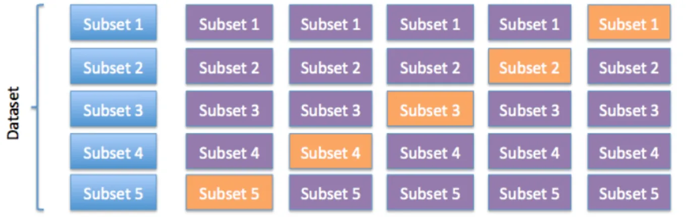
with respect to the rank with p = 200, k = 100 and = 1/100. . . 25 1.8 k-fold cross-validation: with k = 5. The model is iteratively trained on 4/5

(purple) of the data and tested on the remaining 1/5 (orange). The accuracy is thus measured 5 times and finally averaged. . . 28 1.9 The Central Dogma of Molecular Biology. . . 30

(17)

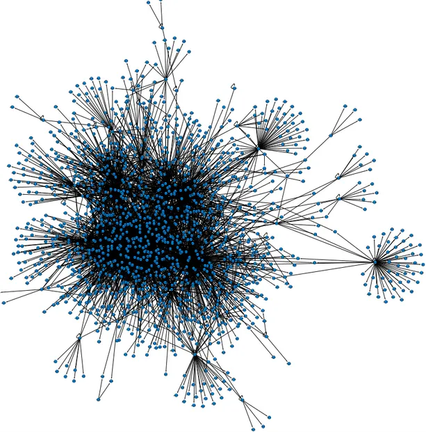
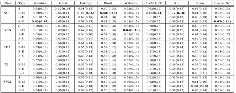
1.10 E. coli regulatory Network: regulation of genes by transcription factors rep-resented as a graph. . . 32 2.1 Area under the ROC curve. Signature of size 100 in a 10-fold CV setting and

averaged over the four datasets . . . 43 2.2 Area Under the ROC Curve. NC classifier trained as a function of the size

of the signature, for diﬀerent feature selection methods, in a 10-fold CV setting averaged over the four datasets . . . 44 2.3 Area Under the ROC Curve. NC classifier trained as a function of the number

of samples in a 50 ⇥ 10-fold CV setting. We show here the accuracy for 100-gene signatures as averaged over the 4 datasets. Note that the maximum value of the x axis is constrained by the smallest dataset, namely GSE2990. . . 45 2.4 Area Under the ROC Curve. NC classifier trained as a function of the number

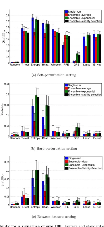
of samples in a 50 ⇥ 10-fold CV setting for each of the four datasets. We show here the accuracy for 100-gene signatures. . . 45 2.5 Stability for a signature of size 100. Average and standard errors are obtained

over the four datasets. a) Soft-perturbation setting. b) Hard-perturbation setting. c) Between-datasets setting. . . 47 2.6 Evolution of stability of t-test signatures with respect to the size of the

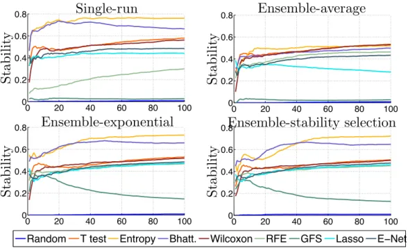
train-ing set in the hard-perturbation and the between datasets setttrain-ings from GSE2034 and GSE4922. . . 48 2.7 Stability of diﬀerent methods in the between-dataset setting, as a function

of the size of the signature. . . 48 2.8 GO interpretability for a signature of size 100. Average number of GO BP

terms significantly over-represented. . . 49 2.9 GO stability for a signature of size 100 in the soft-perturbation

set-ting. Average and standard errors are obtained over the four datasets. a) Soft-perturbation setting. b) Hard-Soft-perturbation setting. c) Between-datasets setting. . 50 2.10 Bias in the selection through entropy and Bhattacharyya distance

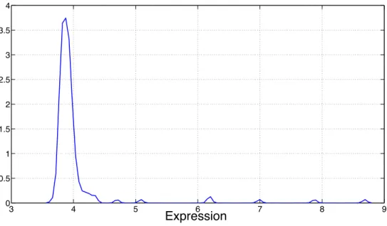
Es-timated cumulative distribution functions (ECDF) of the first ten genes selected by four methods on GSE1456. They are compared to the ECDF of 500 randomly chosen background genes. . . 51 2.11 Estimated distribution of the first gene selected by entropy and

Bhat-tacharyya distance. . . 52 2.12 Accuracy/stability trade-oﬀ. Accuracy versus stability for each method in the

between-datasets setting. We show here the average results over the four datasets. 53 3.1 Stability selection scores for all edges, as a function of . . . 60 3.2 Sg-scores for all edges, as a function of . . . 61

(18)

3.3 Balanced accuracy of the unpenalized logistic regression model trained on the signature selected by the Lasso as a function of the size of the signature. . . 63 3.4 Balanced accuracy of the unpenalized logistic regression model trained on the

signature selected by the Lasso with stability selection, as a function of the size of the signature. . . 64 3.5 Balanced accuracy of the unpenalized logistic regression model trained on the

signature selected by the graph Lasso as a function of the size of the signature. . 64 3.6 Balanced accuracy of the unpenalized logistic regression model trained on the

signature selected by the graph Lasso with stability selection, as a function of the size of the signature. . . 65 3.7 Balanced accuracy on the Wang dataset when selecting the genes on Wang

(green) and Van’t Veer (blue) datasets for the four algorithms. . . 65 3.8 Number of genes present in exactly 1, 2, 3, 4 and 5 of the 5 folds for the four

algorithms. . . 66 3.9 Number of genes present in both the signature generated on the Van’t Veer

and the Wang datasets, as a function of the number of genes considered in the signature. . . 67 3.10 Connectivity index of the signatures as a function of the number of genes

considered in the signature. . . 67 3.11 Signature obtained with the Lasso algorithm. . . 68 3.12 Signature obtained with the graph Lasso algorithm with stability selection. 69 4.1 Convergence of the algorithms. RDG as a function of time for FISTA and

diﬀerent variants of ADMM. All algorithms were run during 5, 000 iterations. Although iterations of FISTA are faster, it converges much slower. Adaptive ADMM seems to be constantly a good choice. . . 81 4.2 Accuracy and stability averaged over the four breast cancer datasets. . . 82 4.3 Absolute correlation and stability averaged over the four breast cancer datasets. 83 5.1 Stability Selection : Illustration of the stability selection frequency F (g, t, L)

for a fixed target gene g. Each curve represents a TF t 2 Tg, and the horizontal axis represents the number L of LARS steps. F (g, t, L) is the frequency with which t is selected in the first L LARS steps to predict g, when the expression matrix is randomly perturbed by selecting only a limited number of experiments and randomly weighting each expression array. For example, the TF corresponding to the highest curve was selected 57% of the time at the first LARS step, and 81% of the time in the first two LARS steps. . . 91

(19)

5.2 Overall Score for Network 1: Top plots show the overall score for R = 4, 000 and bottom plots depict the case R = 10, 000 for both the area (left) and the original (right) scoring settings, as a function of ↵ and L. . . 98 5.3 Optimal values of the parameters : optimal values of parameters L, ↵ and

N with respect to the number ofresampling runs. . . 99 5.4 Impact of the number of resampling runs : overall score as a function of

R. In both scoring settings, ↵ and Lwere set to 0.4 and 2, respectively. . . 100 5.5 Distribution of the number of TFs selected per gene for L=2 :

his-tograms of the number of TFs selected per gene with respect to the total number of predictions when L = 2. . . 101 5.6 Distribution of the number of TFs selected per gene for L=20 :

his-tograms of the number of TFs selected per gene with respect to the total number of predictions when L = 20. . . 102 5.7 Performance on Network 1: ROC (left) and Precision/Recall (right) curves

for several methods on Network 1. . . 103 5.8 Performance on DREAM5 network 3: ROC (Left) and Precision/Recall

(Right) curves for several methods on DREAM5 network 3. . . 103 5.9 Performance on DREAM5 network 4: ROC (Left) and Precision/Recall

(Right) curves for several methods on DREAM5 network 4. . . 104 5.10 In vivo networks results: overall score with respect to L for DREAM5

net-works 3 and 4 and E. coli network (↵ = 0.4, R = 10, 000). . . 104 5.11 Performance on the E. coli network: ROC (Left) and Precision/Recall

(Right) curves for several methods on the E. coli dataset. . . 105 5.12 Spurious edges shortest path distribution: exact distribution of the shortest

path between spuriously predicted TF-TG couples. . . 105 5.13 Distribution of the shortest path with respect to the number of

pre-dictions: distribution of the shortest path length between nodes of spuriously detected edges and 95% confidence interval for the null distribution. These edges are ranked by order of discovery. . . 106 5.14 Distance-2 patterns: the three possible distance-2 patterns: siblings, couple

and grandparent/grandchild relationships. . . 107 5.15 Distribution of distance-2 errors: distribution of distance 2 errors with

re-spect to the number of predictions. 95% error bars were computed using the quantiles of a hypergeometric distribution. . . 108 5.16 Results on DREAM4 networks: overall score on the five multifactorial size

(20)

6.1 Evolution of the number of publications related to feature selection from microarray data until october 2012. . . 120

(21)

(22)

List of Tables

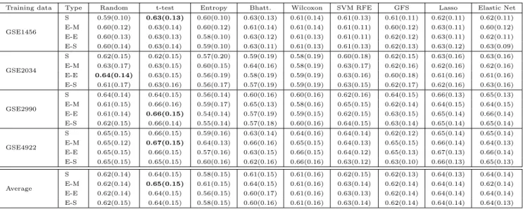
1.1 Classification setting: four necessary measures. TN : True Negatives; FN: False Negatives; FP: False Positives; TP: True Positives. . . 26 2.1 Data . . . 41 2.2 AUC (10-fold cross-validation) . . . 42 2.3 AUC (between-datasets setting) . . . 43 4.1 Data . . . 80 5.1 Datasets: the four datasets used in our experiments. . . 94 5.2 DREAM5 networks results: AUPR, AUROC and minus the logarithm of

related p-values for all DREAM5 Networks and state-of-the-art methods. . . 96 5.3 E. coli network results: TIGRESS compared to state-of-the-art methods on

the E. coli network. Since no p-value can be computed here, the score is simply the average between AUROC and AUPR. . . 102 5.4 DREAM4 networks results: results on the 5 DREAM4 size 100 multifactorial

(23)

(24)

Abstract

Biotechnologies have moved the paradigm of gene expression analysis from a hypothesis-driven to a data-driven approach. Ever since "omics" data have been made available, we are indeed facing a sea of data that we need to mine in order to extract relevant biological information. However, the ease with which it is now possible to obtain genome-wide data is not at all illustrative of the complexity of such data, which is referred to as being high-dimensional.

The technology of DNA microarrays, for example, makes it possible to measure the expression of thousands of genes simultaneously and in several conditions. In this thesis we work on two applications involving microarray expression data: prediction of breast cancer outcome and gene regulatory network inference.

In this thesis, we address these two problems with the same statistical approach, namely the association of supervised learning and feature selection. Supervised learning refers to elucidating patterns linking some data to a response using a set of examples and to using the inferred patterns to predict the response when new data comes along. Feature selection is the process of extracting relevant information from data possibly clouded by high quantities of noise. Among the feature selection methods we discuss, we are interested in the so-called Ensemble methods that consist in incorporating randomization techniques within the selection process through the use of resampling or bootstrap.

Prediction of breast cancer outcome

Being able to predict breast cancer outcome is a pressing issue as the treatment depends on the prognosis. In fact, if there is an indication that a primary cancer will relapse or metastasize, adjuvant chemotherapy after, e.g., a surgery, is the preferred treatment to increase the chances of survival of the patient. However, chemotherapy is only harmful to good outcome patients, i.e., in cases where the cancer is not recurrent. Practicians thus have to estimate the chances of recurrence to decide if and when such adjuvant therapy is necessary. Some clinical and histological factors have been helpful to this task, such as the size and grade of the tumor, the age of the patient or the cancer subtype. However, the accuracy of these indicators is not as

(25)

high as we would hope.

The accessibility of gene expression information through DNA microarrays has opened new perspectives to this problem. In 2002, Van’t Veer and colleagues suggested that mining through microarrays would make it possible to extract molecular signatures predictive of the outcome. A signature consists of a list of a few tens of genes believed to contain necessary and suﬃcient information to assess the likelihood of recurrence of a cancer with some success. These genes are selected based on patterns inferred from the expression profiles of the primary tumor using feature selection methods. The outcome is then predicted through supervised learning models.

This idea appealed to the community and soon tens of new signatures would be published. However, they were only sharing very few genes, if any, which would soon beg questions about the reliability of such models.

The first three chapters of this thesis contribute to this very problem. In Chapter 2, we set up a benchmark in order to compare 32 feature selection methods in light of the accuracy, stability and interpretability of the signatures they find. We show, in particular, that the simplest methods seem to provide the best accuracy/stability trade-off. In Chapter 3, we propose to incorporate biological prior information to the selection procedure using the Graph Lasso with the hope of increasing the stability and interpretability of prognosis signatures. We show that adding such prior information can be useful in terms of interpretation, but does not seem to return more accurate or stable signatures. In Chapter 4, we use a different approach, enforcing structured sparsity through model penalization by the k-support norm, in order to select genes resembling each other without using any prior information. We propose to add two levels of randomization to the algorithm. Our experiments suggest that the resulting method overperforms previously investigated ones in terms of accuracy. Finally, in Chapter 6, we discuss the current state of research in this field, try to look with hindsight at ten years of findings and investigate the apparent trade-off between accuracy and stability.

Inferring Gene Regulatory Networks

The expression of genes is regulated by proteins called transcription factors (TF) that bind to promoter regions and either activate or repress the expression of target genes (TG). Because TFs themselves result from genes being transcribed at some point, the patterns of regulation can be represented on a directed graph, where nodes and edges represent genes and regulation directions, respectively. Such a graph is also called a Gene Regulatory Network (GRN). Understanding TF-TG interactions has many potential applications in biology and medicine, ranging from in silico modeling and simulation of GRN to the identification of new potential drug targets.

GRN inference can be seen as a series of supervised learning tasks, where the expression of each TG is predicted by the expression of the TFs regulating it. A typical assumption is the sparsity of these networks, in that only few TFs are believed to regulate a TG. Therefore, feature

(26)

selection can be used to detect the set of TFs interacting with each TG.

It is this approach that we choose to follow in Chapter 5. We describe an algorithm named TIGRESS, with which we participated into the DREAM5 GRN inference challenge. DREAM stands for Dialogue on Reverse Engineering Assessments and Methods and proposes yearly challenges on various biological problems. The GRN inference challenge consisted in inferring three networks, i.e., in predicting probabilities of existence for each edge in each of the three networks. TIGRESS ranked second in the in silico network sub-challenge and third overall. The algorithm is based on a popular `1-penalized method called Lasso on top of which we added two randomization layers. In Chapter 5, we analyze the behavior of the algorithm in various situations, assess the impact of the choice of its parameters and benchmark it against state-of-the-art GRN inference methods. Our results are extremely encouraging as to the ability of such machine learning-based approaches to solve the GRN inference problem and that of TIGRESS, in particular.

(27)

(28)

Résumé

De considérables développements dans le domaine des biotechnologies ont modifié notre approche de l’analyse de l’expression génique. En eﬀet, s’il était auparavant nécéssaire de formuler une hypothèse - concernant un gène, par exemple - pour pouvoir la tester, c’est la démarche inverse que l’on suit depuis l’apparition, il y a une quinzaine d’années, des données "omics". Il s’agit désormais d’extraire l’information à partir d’une grande quantité de données, et il est finalement devenu bien plus simple d’obtenir des informations quantitatives à l’échelle du génome que de les analyser. On parle alors de données en grande dimension.

Les puces à ADN sont un exemple de ce phénomène. Elles permettent de mesurer l’expression de milliers de gènes de manière simultanée et dans diﬀérentes conditions. Dans cette thèse, nous travaillons sur deux applications impliquant l’analyse de telles données : la prédiction de l’issue du cancer du sein et l’inférence de réseaux de régulation génique.

Bien que ces deux problèmes ne semblent, a priori, rien avoir en commun, nous les approchons par la même démarche statistique, à savoir l’association de l’apprentissage supervisé et de la sélection de variables. L’apprentissage supervisé consiste, à partir d’un ensemble d’exemples, à repérer, ou apprendre des liens entre des données et une réponse, de manière à pouvoir prédire la réponse lorsque de nouvelles données se présentent, en utilisant les règles apprises. La sélection de variables se rapporte à un ensemble de méthodes permettant d’extraire l’information importante d’une base de données parfois très complexe et potentiellement corrompue par beaucoup de bruit. Parmi les techniques de sélection de variables, nous nous intéressons, entre autres, aux méthodes dites d’ensemble, qui consistent à incorporer une part de randomisation au processus de sélection, par le biais du ré-échantillonnage ou du bootstrap.

Prédiction de l’issue du cancer du sein

Le traitement du cancer du sein étant dépendant du pronostic, il est capital d’être en mesure de prédire l’issue de la maladie. En eﬀet, si l’on suspecte qu’un cancer primaire donnera lieu à une métastase ou une récurrence, on peut proposer à la patiente une chimio-thérapie adjuvante, c’est-à-dire à la suite d’une opération chirurgicale. Dans de tels cas, ce type de traitement,

(29)

destiné à accroître l’espérance de vie de la patiente, est nécessaire. En revanche, dans le cas où le cancer disparaît après l’intervention, la chimio-thérapie est néfaste à la patiente, attaquant uniquement des cellules saines. Les médecins doivent donc estimer la probabilité de récurrence du cancer afin de décider si un tel traitement adjuvant est nécessaire. Des facteurs cliniques et histologiques donnent un certain nombre d’indications et sont un appui pour le pronostic. Cependant, la capacité prédictive de ces estimateurs reste faible.

L’accès aux données d’expression des gènes, grâce à des techniques telles que les puces à ADN, ont ouvert de nouvelles perspectives à ce problème. En 2002, une étude suggérait que de nouveaux indicateurs pouvaient être obtenus en analysant ces puces. Il s’agit d’extraire de ces données ce qu’on appelle des signatures moléculaires. Une signature est une liste de quelques dizaines de gènes supposée contenir suﬃsamment d’information liée au pronostic et qui permettrait donc de calculer la probabilité de récurrence du cancer pour de nouvelles pa-tientes. Ces gènes sont sélectionnés à partir de profils d’expression géniques de la tumeur primaire grâce à des méthodes de sélection de variables. L’issue est alors prédite par le biais de modèles d’apprentissage supervisé.

Cette idée eut immédiatement de l’écho dans la communauté, de telle manière que, très vite, des dizaines de nouvelles signatures furent publiées. Cependant, on se rendit compte qu’elles n’avaient que peu de gènes en commun, ce qui remit en question la fiabilité de ces modèles.

Les trois premiers chapitres de cette thèse sont consacrés aux signatures moléculaires pour le pronostic du cancer du sein. Dans le Chapitre 2, nous proposons une comparaison systématique de 32 méthodes de sélection de variables, du point de vue de leur performance prédictive, de leur stabilité et de leur interprétabilité. En particulier, nous montrons que les méthodes les plus simples semblent fournir le meilleur compromis performance/stabilité. Dans le Chapitre 3, nous proposons d’incorporer à la procédure de sélection de l’information biologique a priori par le biais du Graph Lasso, dans l’espoir d’accroître la stabilité et l’interprétabilité des signatures. Nous montrons que si l’ajout d’une telle information permet, en effet, d’obtenir des signatures plus interprétables, cela ne semble, en revanche, pas avoir d’effet sur la performance ou la stabilité. Dans le Chapitre 4, nous utilisons une approche différente, à savoir la parcimonie structurée, à travers un modèle pénalisé par la norme dite "k-support", dans le but de sélectionner des gènes qui se ressemblent sans cependant utiliser d’information a priori. Nous proposons, par ailleurs, d’ajouter deux niveaux de randomisation à la sélection. Il semble, à première vue, que cette approche permette d’accroître la performance des signatures par comparaison aux techniques déjà évaluées. Enfin, dans le Chapitre 6, nous exposons l’état actuel de la recherche dans ce domaine et tentons de prendre du recul sur plus de dix années de publications.

(30)

Inférence de réseaux de régulation

L’expression des gènes est régulée par des protéines appelées facteurs de transcription (TF), qui, en se fixant sur des séquences en amont des gènes cibles (TG), activent ou répriment leur transcription. Les TFs résultant eux-mêmes de gènes ayant été transcrits, ces relations entre gènes peuvent être représentées sur un graphe dirigé, où les noeuds et les arètes représentent respectivement les gènes et les interactions TF-TG. Un tel graphe est appelé réseau de régulation génique (GRN). La connaissance et la compréhension des interactions TF-TG ont de nombreuses applications, de la modélisation et la simulation de réseaux in silico à l’identification de nouvelles cibles thérapeutiques potentielles.

L’inférence des GRNs à partir de données de puces peut être approchée statistiquement comme une série de tâches d’apprentissage supervisé, où l’expression de chaque TG est prédite par l’expression des TFs le régulant. Une hypothèse couramment admise est la parcimonie de ces réseaux: on suppose que seul un petit nombre de TFs régule un TG. Il s’agit donc également d’un problème de sélection de variables où le but est d’identifier l’ensemble des TFs interagissant avec chaque TG.

Nous adoptons cette approche dans le Chapitre 5. Nous y décrivons un algorithme nommé TIGRESS, avec lequel nous avons participé au challenge d’inférence de réseaux DREAM5. DREAM (Dialogue on Reverse Engineering Assessemnts and Methods) propose chaque année des challenges portant sur diﬀérentes questions biologiques. Le problème d’inférence de GRNs consistait à prédire les probabilités d’existence des arètes pour trois réseaux, à partir de données d’expression. TIGRESS a été classée seconde sur le réseau in silico et troisième dans l’ensemble. L’algorithme est basé sur le Lasso, une méthode de pénalisation utilisant la norme `1, à laquelle nous avons ajouté deux niveaux de randomisation. Dans le Chapitre 5, nous analysons le po-tentiel et les limites de cette méthode dans diﬀérentes situations, nous évaluons l’impact de ses paramètres et nous la comparons à l’état de l’art. Les résultats sont très encourageants, validant l’intérêt d’utiliser des méthodes d’apprentissage pour l’inférence des GRNs, et de TIGRESS en particulier.

(31)

(32)

Chapter

1

Introduction

In this chapter, we aim at providing some mathematical and methodological background on two main concepts present in this thesis, namely supervised learning and feature selection.

Supervised learning is concerned with the inference of a rule that links some input and output data. The inference is performed on training samples for which we are given the output, or the response. The aim is to use the learned rule to predict the response when new input data is given. The problem of breast cancer outcome prediction, for example, amounts to understanding the relation between the expression of genes and the metastatic status of the cancer. Detailed overviews on supervised learning are given in, e.g.,Vapnik (1998), Hastie et al. (2009),Bishop

(2006).

Feature selection consists in mining the entire dataset with the goal of identifying the relevant variables, with respect to the problem at hand. Feature selection can be performed either through subset selection, i.e., by seeking the best group of features among those available, or through feature ranking that consists in ordering the variables by their importance. References on feature selection methods include Guyon and Elisseeﬀ(2003),Liu and Motoda (2007).

This chapter is organized as follows. Section 1.1 provides a general introduction to supervised learning and introduces the concept of regularization. Section 1.2 is concerned with feature selection and feature ranking. In Section 1.3, we provide guidelines to correctly evaluate and compare models. Finally, Section 1.4 provides an overview of the contributions of this thesis.

1.1 Supervised learning to predict and understand

As generally as it gets, machine learning can be defined as a set of powerful tools to make sense of data. Through modeling and algorithms, one major goal of the discipline is to extract interesting patterns from the data and take advantage of them to make sensible decisions.

In this thesis, we focus on supervised learning, where the response to a specific question is known for a given set of observations called training set and the aim is to predict the response

(33)

when new input is given. When the response is discrete, i.e., encoded as classes, the problem is called classification. On the other hand, real responses call for regression models and algorithms. This section first introduces supervised learning in a very general way. We then discuss two important concepts in this field, referred to as the approximation/estimation trade-oﬀ and the accuracy/interpretability dilemma. The last part of this section focuses on a particular type of models, called penalized methods.

1.1.1 Supervised machine learning: problem and notations

The input data consists in n observations, each described by a set of p features. In the remaining, we will denote the observations by (xi)i=1...n, where for all i, xi _{2 X ✓ R}p. Concretely, we observe a matrix X = (xi,j)i=1...n,j=1...p consisting of n lines and p columns.

The output data, or response is described a vector Y = (yi)i=1...n. In a classification setting, the response consists of C classes: Y 2 {1...C}n_{. In the particular case of binary classification,} Y _{2 { 1, +1}}n_{. In a regression setting, the response is a continuous variable: Y 2 R}n_{. For} instance, predicting the outcome of breast cancer is a binary classification problem, with yi specifying the outcome (yi = +1 in case of a metastatic event, and 1 otherwise). Predicting the expression level of a gene is a regression problem (expression yi2 R). For the general case, we write that yi2 Y ✓ R for all i.

Pairs (xi, yi)i=1...nare realizations of the random variables (Xi, Yi)i=1...n assumed to be i.i.d. from the same unknown joint distribution P of (X, Y ).

We aim at predicting Y from X, i.e., we seek a function f belonging to some set F := {f : X ! R, f measurable}, that we will call a predictor, such that ˆY := f (X)is close to Y , in some sense. The distance between f(X) and Y is measured by a loss function l : R ⇥ Y ! R+. The smaller l(f(X), Y ), the better the prediction. The performance of f is measured as the expected loss over P, called Risk:

Rl(f ) = EP[l(f (X), Y )]. (1.1) The best f is thus obtained by solving the following risk functional minimization problem (Vapnik,1995)

f⇤ = arg min

f2FRl(f ). (1.2)

However, the distribution P is unknown and the risk Rl(f ) is thus not computable. (1.1) is therefore estimated by the empirical risk:

ˆ Rl(f ) = 1 n n X i=1 l(f (xi), yi)

and f⇤ _{in equation (1.2) approximated by:} ˆ

f = arg min

f2F

ˆ

(34)

This program is known as the empirical risk minimization.

The first question that arises relates to the choice of l. The second issue is to decide how the set of possible functions F should be defined.

1.1.2 Loss functions

We are interested in convex problems (Boyd and Vandenberghe,2004) and therefore require that f ! l(f(x), y) be convex for all (x, y) 2 X ⇥ Y.

Square loss

The square loss function is defined as

lsq(f (x), y) = (y f (x))2.

It is mainly used in regression problems, such as the least squares regression but can also be used in a classification problem. One major advantage of this loss is that it is diﬀerentiable everywhere. However, a typical flaw of the square loss is that outliers are heavily penalized, and these penalties enormously aﬀect the empirical risk and hence the answer.

Logistic loss

Commonly used for classification purposes, the logistic loss is llog(y, f (x)) = ln(1 + exp( yf (x))).

The empirical risk of the logistic loss corresponds to the log-likelihood of the logistic regression (Menard, 2001), where it is assumed that p(Y = 1|X) = 1

1+exp( f (X)) = 1 1+exp(f (X))1 =

1 p(Y = 1_{|X). Therefore, we also have p(Y = y|X) =} _{1+exp( yf (X))}1 for y 2 { 1, +1}. Hinge loss

In a classification setting, the hinge loss can also be used:

lhin(y, (f (x))) = max(0, 1 yf (x)).

It should be interpreted from the Support Vector Machine (Vapnik,1995) viewpoint where yf (x) corresponds to the margin that we want to maximize. When f(x) is on the correct side of the separator, i.e., when sgn(f(x)) = sgn(y) and the margin is greater than 1, there is no price to pay. Otherwise, the smaller the margin, the larger the (linear) cost.

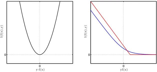
Figure 1.1 depicts these three loss functions: the left panel shows the square loss as a function of y f(x) while the left panel focuses on the classification setting and depicts the logistic and hinge losses. On the latter, we can see how the logistic loss behaves as a softer version of the hinge loss.

(35)

0 0 yf(x) l( f( x ),y ) 0 0 y-f(x) l( f( x ),y )

Figure 1.1: Loss functions. The left panel shows the square loss. The logistic (blue) and hinge (red) losses are depicted on the right panel.

1.1.3 Defining the complexity of the predictor

Recall that we are looking for the function f that minimizes the empirical risk. We show a two-class classification example on Figure 1.2.

Figure 1.2: Binary classification problem and overfitting. The aim to separate the two classes can be achieved with more or less complexity. The dotted separator fits the data perfectly but is prone to generalizing poorly. The plain linear separator, on the other hand, allows some training points to be misclassified but will fit new data in a more general and interpretable way. Each of the two lines depicts a way to separate the blue class and the orange one. The question that we address here is: "which of the two separators is the best?". In this case, there are two main reasons why one should choose the plain simpler classifier. The so-called approximation/estimation trade-oﬀ is the first and most crucial of them as we develop below.

(36)

Depending on the problem, one may also care about the interpretability of the solution, which we will discuss as well.

Approximation error and estimation error

One should always keep in mind that the end game is to classify correctly new data (Vapnik and Chervonenkis, 1974). A classifier that yields no error on the training set - possibly noisy and containing outliers - is therefore not necessarily the best choice, as it may generalize poorly to new points. This behavior is known as over-fitting. Another way to see this is to look at the stability of the classifier: if one point were to be changed in the training set, how much would it aﬀect the separation? Taking a look at Figure 1.2, we guess that the direction of the plain line would only be slightly modified, if at all. The dotted separator, however, might just surprise us with a very diﬀerent shape, should one blue point, for the sake of argument, be moved into the middle of the orange crowd.

Formally, there is a need to introduce restrictions on f. This is done by searching over some set H ⇢ F. Obviously, the chance that f⇤ _{2 H is extremely small. Therefore, the new goal is} to find the best possible function f⇤

H2 H: f_H⇤ = arg min f2HRl(f ). (1.4) It is estimated by ˆ f_H= arg min f2H ˆ Rl(f ). (1.5)

The error made by restricting the set of possible functions is referred to as the approximation error or, with somewhat of a misuse of language, the bias.

The estimation error of the predictor refers to the diﬃculty of estimating f⇤

Hand is sometimes referred to as the variance.

Constraining the set will increase the approximation error, as chances are high that the true predictor f⇤ _{2 H. However, it will make the estimation easier to control and thus reduce the}_/ estimation error. On the other hand, the less we constrain f, the closest our model to the true underlying model assumed to have generated the data. But in this case, we risk having diﬃculties estimating it.

This trade-oﬀ is often referred to as the approximation/estimation dilemma - and, with some misuse of language, to the bias/variance dilemma - and is illustrated on Figure 1.3 where the total error is decomposed into the bias and the variance terms:

total error = Rl(f_H) Rl(f⇤) = Rl(fH) Rl(f_H⇤) | {z } estimation error + Rl(f_H⇤) Rl(f⇤)] | {z } approximation error

(37)

Figure 1.3: Approximation error and estimation error. The error made when choosing ˆf_H to estimate f⇤ _{can be seen as the sum of bias and variance. The bias refers to the approximation} error and the variance to the estimation error.

This trade-oﬀ is a crucial concept in machine learning with enormous consequences. One way to reduce, if not overcome it, is to think of H as a set constraints, which leads to the definition of penalized methods, that we describe in section 1.1.4. By forcing the objective function to meet some constraints, we achieve our goal to restrict the search. We explain in Section 1.1.4 how it can be done in a way that allows us to take into account specificities of our problem.

The interpretability/accuracy dilemma

Although not always a critical point, outputting an interpretable solution can be a requirement in some applications. Breast cancer prognosis, for example, is about predicting the probability of a metastatic event. If the model that does that can also make biological sense, interdisciplinary applications are made easier by joining forces to understand the phenomenon. Indeed, assuming one can produce a model that, on top of being performant, makes it clear how much a given gene is involved in breast cancer outcome and in what way, specific biological experiments can be carried out with a higher chance of discovering important patterns. Deciding which variables are relevant is the focus of feature selection as we will develop in Section 1.2.

This being said, there is no denying that we might be facing particularly complex systems. For example, systems biology studies biological properties whose elaboration might just go be-yond our understanding. Leo Breiman argues in Breiman (2001b) that, in many cases, data models are not necessarily the right choice. Data modeling consists in assuming a model (linear, logistic, ...) and then infer its parameters. They can be put in opposition to algorithmic models where the only assumption is that by some function f that we do not know a thing about, X becomes Y . On problems involving gene expression data, Breiman writes:

It requires that [the statisticians] focus on solving the problem instead of asking what data model they can create. The best solution could be an algorithmic model, or maybe a data model, or maybe a combination. But the trick to being a scientist is to

(38)

be open to using a wide variety of tools.

He advertises for black boxes such as random forests (Breiman,2001a), Neural Networks (Bishop,

2006) or Support Vector Machines (Vapnik,1995), acknowledging that these algorithms are only slightly more interpretable than nature’s black box itself and that the most accurate methods are the less interpretable ones. "The goal is not interpretability", he writes, "but accurate information".

This apparently leaves us with a choice: in an eﬀort to provide both accurate predictions and some understanding to complex biological systems, we might have to choose between the two.

In this thesis, we combine data and algorithmic models in the sense of Breiman: starting with simple assumptions, e.g., with a parametric model, we find it necessary to introduce ran-domness. In particular, we will make intensive use of tools such as bootstrap (Efron,1979) and bagging to build Ensemble algorithms for feature selection, as developed in Section 1.2.5. In the remaining, we will pay particular attention to investigating the interpretability/accuracy dilemma. In Section6.3, we re-discuss this issue in light of the results presented in the core of this document.

1.1.4 Penalized methods

In the previous section, we introduced the idea of constraining the objective function to a restrained set H. From now on, we will consider objectives that depend on a linear combination of the covariates, i.e., f(X) = X! where ! is a vector of weights in Rp_{. Note that, e.g., the} linear and the logistic models belong to this class of functions:

Linear Y = X! + ", " i.i.d. N (0, 2₎ Logistic P(Y = 1|X) = exp( X!)

1+exp( X!)

Constraining f now amounts to constraining !, i.e, equation (1.3) becomes: (

ˆ

! = arg min_!2RpRˆ_l(!)

s.t. ⌦(!)  T (1.6)

where ⌦ : Rp _{! R is a penalty. If ˆ}_R

l and ⌦ are both convex and under weak additional assumptions (see, e.g., Boyd and Vandenberghe,2004, Section 5.2), (1.6) can be written in its Lagrangian form: ˆ ! = arg min !2Rp ˆ Rl(!) + ⌦(!) (1.7)

Both and T control the amount of regularization: when increases (resp. when T de-creases), the weights ! are more penalized. When = 0 (resp. T = +1), the model is not penalized.

(39)

Depending on the problem, we may want to impose specific conditions on these weights, i.e., specific forms for ⌦. In the following, we expose some of these conditions and try to give insight as to when they make sense. More detailed overviews of regularized methods can be found in, e.g.,Huang et al. (2009),Bach et al. (2011a).

Enforcing smoothness: `2 regularization

A common example of a constrained problem is the Tikhonov regularization (Tikhonov, 1963), also known as Ridge regression: assume a classical linear setting Y = X! + ". If the design of X makes it possible to invert XTX, the Ordinary Least Squares (OLS) solution is:

ˆ

!OLS = arg min

!2Rp||Y X!||

2

2 = (XTX) 1XTY. (1.8) This model, however, is not always an option, in particular when the number p of variables exceeds the number of examples n, making the matrix XT_X _{singular. Ridge regression (}_Hoerl

and Kennard,1970) consists in adding the regularization function ⌦(!) = ||!||2

2to the empirical risk:

ˆ

!Ridge= arg min

!2Rp||Y X!||

2

2+ ||!||2 = (XTX + Ip) 1XTY. (1.9) The first consequence is numerical: for any > 0, XT_{X + I}

p becomes invertible, indepen-dently of the initial design. Second, and most importantly, it enforces the smoothness of the functional, in the sense of Lipschitz. Indeed, the larger , the smaller the Lipschitz constant ||!||2 in the following equation:

||f(x1) f (x2)||2 =||x1! x2!||2  ||!||2||x1 x2||2. (1.10) Equation (1.10) is extremely valuable from the machine learning point of view: the smooth-ness of f seems to solve at least the first of the two dilemmas presented in Section 1.1.3. Indeed, when predicting the output y from a new point x, provided it is close - in the sense of the euclidian distance - to some point xtr in the training set, we make sure that our prediction ˆy will be close to ytr. The variance of the prediction is therefore reduced, leaving us with only the bias to control. In a sense, we may also see the Ridge penalization as a help to the interpretability issue: because the Ridge solution is more stable, i.e., diﬀerent training sets should lead to similar solutions provided they themselves are similar. It might thus be reasonable to assume that large values of ˆ! correspond to important covariates.

An interesting interpretation is provided by Bayesian statistics, that consider the penalty as a prior distribution on !: assume that p(!) = N (0,1_I

p) and p(Y |X, w) = N (Xw, 2). Then maximizing the joint likelihood is equivalent to solving problem (1.9). Indeed, assuming = 1:

(40)

L(X, Y, !) = exp( 1 2||Y X!|| 2 2 ₂||!||22) / exp ⇢ 1 2(! X T_Y)T 1_(! _XT_Y)

where = (XTX + Ip) 1. We thus recover the posterior distribution of !: !|X, Y N ( XT_Y, ₎_{. The maximum a posteriori (MAP) is therefore the mean} _XT_Y_, correspond-ing to the Ridge solution (1.9). We can see now how increascorrespond-ing will yield an estimator with both a smaller mean and a smaller variance.

The `2 regularization is best known in the regression setting. However, it has also been studied in the classification setting (Hastie et al., 2009), and in particular in the context of support vector machines (Vapnik,1995).

Enforcing sparsity: `1 regularization

Ridge regression constrains the amplitude of the weights in the linear model. However, it does not account for the possible sparsity of the data. In recent years, technological progresses have reversed some of the problems faced by the statistical community: it appears that acquiring information on a huge set of variables has been made easier than deciding which variables to experiment with. This seems especially true in bioinformatics, where the behavior of thousands of genes can be evaluated at a cost similar to that of just a few. This new situation makes our approach a little diﬀerent as, in many cases, we can safely assume that only some of the genes are relevant to the problem at hand, the rest just being noise. Under these considerations, it seems only appropriate that the predictor be sparse, i.e., the goal is to return a vector ! with only a few non-zero entries relating to the relevant variables.

In this section, we introduce the earliest and still most popular method that enforces sparsity on the weights by penalizing their `1 norm, namely the Lasso regression.

Recall that the `1 norm is defined as ||x||1=

p X j=1

|xj|. (1.11)

The Lasso regression (Tibshirani, 1996) or basis pursuit (Chen et al., 1998) is done by regularizing the weights by ⌦(!) = ||!||1:

ˆ

!Lasso = arg min

!2Rp||Y X!||

2

2+ ||!||1 (1.12)

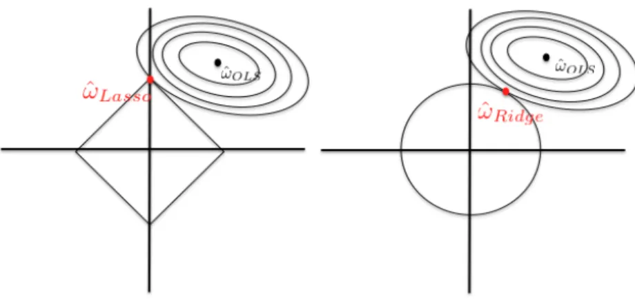
Controlling the sum of absolute values will have a diﬀerent eﬀect than controlling the sum of squares (`2 norm). As shown in Figure 1.4, the `1 norm induces sparsity whereas the `2 norm only reduces the amplitude of the weights.

(41)

Figure 1.4: Lasso and Ridge regressions. In order to fit the constraint, the loss (here the square loss represented by its elliptical curves) approaches the boundaries of the ball. In the `1 penalization case, it will likely hit a singularity, forcing the solution to be sparse - in the picture, the first component of ! is zero. When we consider the `2norm, neither component will be zero, almost surely.

Although Lasso was originally introduced as a regression method, penalization by the `1 norm has drawn a lot of attention in many communities. In particular, theoretical properties have been studied for the classification setting. This penalization can thus be used with other types of loss functions, including the logistic loss (Shevade and Keerthi,2003,Koh et al.,2007). In section 1.2.4, we will further discuss the Lasso as a feature selection method and will provide guidelines as to the choice of the penalty parameter .

Enforcing structured sparsity: `1, `2 and beyond

Lasso regularization appeared as a breakthrough to the statistical community. However, one main pitfall of the algorithm is its undesirable behavior when covariates are correlated. This problem is formally known as the irrepresentable condition (Zhao and Yu, 2006). Consider-ing cases where the number of covariates is large - in particular, larger than the number of observations -, there is a high probability that this happens. This is particularly true in the applications that we address: not only are the genes suspected to be correlated, many happen to be biologically linked in a causal way.

When the Lasso is faced with such a correlated design, it will generally choose one covariate among the set of correlated ones and set the others to zero. Ran several times, it might even choose a diﬀerent variable each time. The reason for that is given intuitively in the following result from Zou and Hastie(2005):

Suppose the extreme case where for some i and j in {1...p}, Xi = Xj and consider the problem ˆ! = arg min!||Y X!||2

2+ ⌦(!). Then: 1. If ⌦(.) is strictly convex, ˆ!i = ˆ!j

(42)

2. If ⌦(!) = ||!||1, then ˆ!i!ˆj 0 and !⇤ defined by: !⇤_k= 8 > > < > > : ˆ !k if k6= i, k 6= j s.(ˆ!i+ ˆ!j) if k = i (1 s).(ˆ!i+ ˆ!j) if k = j is also a solution to the problem with some s 2 [0, 1]

This result emphasizes two important facts: first, the solution to the Lasso is highly unstable, especially in such a case as high correlation between some covariates. Second, it does not guarantee that similar covariates will receive similar weights. With this problematic in mind,

Zou and Hastie(2005) proposed an improved version of the Lasso, named Elastic Net.

Managing correlated variables : the Elastic Net The Elastic Net appears as a compro-mise between the `1 and `2 regularizations and as such has the advantage of yielding a solution that is both sparse and smooth.

The problem to solve is as follows: !enet = arg min

!2Rp||Y X!||

2

2+ 1||!||1+ 2||!||22 (1.13)

When 2 > 0 the penalty is strictly convex, ensuring the uniqueness of the solution. The following result fromZou and Hastie(2005) sheds light on the behavior of Elastic Net when the design exhibits some correlations:

Let ⇢ = corr(Xi, Xj) for some (i, j) 2 {1 . . . p}2. Assume !ienet!jenet> 0. Then, 1 ||Y ||1|! enet i !enetj |  1 2 p 2(1 ⇢)

Note that when Xi = Xj, that is when ⇢ = 1, we do have ˆ!_ienet = ˆ!enet_j . Moreover, this result overall confirms the grouping eﬀect of the Elastic Net: whereas the Lasso estimate would only select one of the covariates in a correlated group, the Elastic Net selects all of them.

The Elastic Net problem can in fact be seen as a Lasso-like problem. Indeed, it can be written as:

!enet= p 1 1 + 2

!⇤

where !⇤ _{is defined as:}

!⇤ = arg min ! ||Y ⇤ _X⇤_!_||2 2+p 1 1 + 2||!||1 with X⇤ ₌ _p 1 1+ 2 X p 2Ip !

a matrix of size (n + p) ⇥ p and Y⇤ ₌ Y 0

!

a vector of size n + p.

(43)

Thus, the Elastic Net estimate can be computed using an algorithm that solves the Lasso. However, the estimate as described here might enjoy some performance improvements. Indeed, the authors note that, as empirical evidence confirms, the Elastic Net procedure happens in two steps, each of which introduces unnecessary bias and variance. A way to avoid this is to rescale the estimator as:

!enet_improved=p1 + 2!⇤ = (1 + 2)!enet

Adding prior knowledge on grouping: the Group Lasso Given particular problems, one might wish to perform a Lasso-like selection among predefined groups of variables, as opposed to individual features (Lasso) or correlation-built groups (Elastic Net). For instance, a prior knowledge on the interaction of some genes might lead one to consider them together.

In Yuan and Lin(2006), the authors propose an extension to factor selection, introducing a generalization of the Lasso they call Group Lasso.

Consider the following regression problem: Y =

G X g=1

Xg!g+ " (1.14)

where Xg is of size n ⇥ pg and !g of size pg⇥ 1 for all g = 1...G such thatPGg=1pg = p. Each Xg now represents a group g of pg variables. Note that these groups do not overlap.

Note that the particular case pg= 1 for all g, (1.14) we are back to the usual setting. The Group Lasso stands as a generalization of the Lasso procedure considering block penal-ization of these grouped variables:

!GLasso= arg max

! ||Y G X g=1 Xg!g||2+ G X g=1 (!_gTKg!g)1/2 (1.15) where Kg is a pg⇥ pg matrix representing some relation between the variables in group g.

This penalty enforces sparsity at the group level: some ||!g|| will be set to zero, forcing all variables in g to have a zero weight as well.

Not unlike the Elastic net, the penalty ⌦(w) =PGg=1(!TgKg!g)1/2 stands as a compromise between the `1 and the `2 norms, the major diﬀerence being that here the groups are predefined. The authors note that one should be careful with the choice of K.. They choose to set them to Kg = pgIpg in order to balance the (groups of) parameters according to their dimension without

giving one coordinate any special importance within a group. However one could easily imagine choosing these matrices according to some prior knowledge on the variables. In particular, the oﬀ-diagonal terms might be chosen according to the correlation between some covariates within a group.