Developments on Product Propagation
Abdallah Saffidine∗and Tristan Cazenave†
LAMSADE, Université Paris-Dauphine
Abstract. Product Propagation (PP) is an algorithm to backup
proba-bilistic evaluations for abstract two-player games. It was shown thatPP
could solve go problems as efficiently as Proof Number Search (PNS). In this paper, we exhibit a few domains where, for generic non-optimized versions,PPperforms better than previously known algorithms for solv-ing games. The compared approaches include alpha-beta search, PNS, and Monte Carlo Tree Search. We also extendPPto deal with its mem-ory consumption and to improve its solving time.
1
Introduction
Product Propagation (PP) is a way to backup probabilistic information in a two-player game tree search [28]. It has been advocated as an alternative to minimaxing that does not exhibit the minimax pathology [20, 2, 3, 11, 12].
PPwas recently proposed as an algorithm to solve games, combining ideas from Proof Number Search (PNS) and probabilistic reasoning [29]. In Stern’s pa-per,PPwas found to be about as performant asPNSfor capturing go problems.
We conduct a more extensive study of PP, comparing it to various other paradigmatic solving algorithms and improving its memory consumption and its solving time. Doing so, we hope to establish thatPPis an important algorithm for solving games that the game search practician should know about. Indeed, we exhibit multiple domains in whichPPperforms better than the other tested game solving algorithms.
The baseline game tree search algorithms that we use to establishPP’s value are Monte Carlo Tree Search (MCTS) Solver [34] which was recently used to solve the game of havannah on size 4 [9];PNS[1, 31, 14]; and αβ [21].
The next section deals with algorithms solving two-player games. The third section is about the Product Propagation algorithm. The fourth section details experimental results and the last section concludes.
2
Solving two-player games
We assume a deterministic zero-sum two-player game with two outcomes and sequential moves. Game tree search algorithms have been proposed to address
∗
†
games with multiple outcomes [7, 22], multi-player games [30, 25, 19], non-deterministic games [10], and games with simultaneous moves [24].
A generic best-first search framework is presented in Algorithm 1. To in-stantiate this framework, one needs to specify a type of information to asso-ciate to nodes of the explored tree as well as functions to manipulate this type: info-term, init-leaf, select-child, update.
PNSis a best-first search algorithm which expands the explored game tree in the direction of most proving nodes, that is, parts of the tree which seem easier to prove or disprove.
MCTS Solver is also a best-first search algorithm which can be cast in the mentioned framework. In MCTS [6], the information associated to nodes is in the form of sampling statistics, and bandit-based formulas [15] are used to guide the search. The sampling performed at a leaf node inMCTScan take the form of games played randomly until a terminal position, but it can also be the value of a heuristical evaluation function after a few random moves [17, 33]. We denote the latter variant as MCTS-E.
3
Probability Search
3.1 The Product Propagation Algorithm
Product Propagation (PP) is a recently proposed algorithm to solve perfect in-formation two-player two-outcome games based on an analogy with probabili-ties [29].
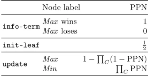
InPP, each node n is associated to a single number PPN(n) (the probabil-ity propagation number for n) such that PPN(n) ∈ [0, 1]. The PPN of a leaf corresponding to a Max win is 1 and the PPN of a Max loss is 0. PPN(n) can intuitively be understood as the likelihood of n being a Max win given the par-tially explored game tree. With this interpretation in mind, natural update rules can be proposed. If n is an internal Min node, then it is a win for Max if and only if all children are win for Max themselves. Thus, the probability that n is win is the joint probability that all children are win. If we assume all children are independent, then we obtain that the PPN of n is the product of the PPN of the children for Min nodes. A similar line of reasoning leads to the formula for Max nodes. To define the PPN of a non-terminal leaf l, the simplest is to assume no information is available and initiate PPN(l) to 12. These principles allow to induce a PPN for every explored node in the game tree and are summed up in Table 1.
Note that this explanation is just a loose interpretation of PPN(n) and not a formal justification. Indeed, the independence assumption does not hold in practice, and in concrete games n is either a win or a loss for Max but it is not a random event. Still, the independence assumption is used because it is simple and the algorithm works well even though the assumption is usually wrong.
To be able to use the generic best first search framework, we still need to specify which leaf of the tree is to be expanded. The most straightforward
ap-bfs(state q, player m) r ← new node with label m r.info ← init-leaf(r) n ← r
while r is not solved do while n is not a leaf do
n ← select-child(n) extend(n)
n ← backpropagate(n) return r
extend(node n)
switch on the label of n do case terminal
n.info ← info-term(n) case max
foreach q0 in {q0, q−→ qa 0} do n0 ← new node with label min n0.info ← init-leaf(n0) Add n0 as a child of n case min
foreach q0 in {q0, q−→ qa 0} do n0 ← new node with label max n0.info ← init-leaf(n0) Add n0 as a child of n
backpropagate(node n) new_info ← update(n)
if new_info = n.info ∨ n = r then return n else
n.info ← new_info
return backpropagate(n.parent )
Algorithm 1: Pseudo-code for a best-first search algorithm.
Table 1. Initial values for leaf and internal nodes inPP. C denote the set of children. Node label PPN
info-termMax wins 1
Max loses 0 init-leaf 12 update Max 1 − Q C(1 − PPN) Min Q CPPN
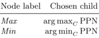
proach is to select the child maximizing PPN when at a Max node, and to select the child minimizing PPN when at a Min node, as shown in Table 2.
Table 2. Selection policy forPP. C denotes the set of children. Node label Chosen child
Max arg maxCPPN Min arg minCPPN
3.2 Practical improvements
The mobility heuristic provides a better initialization for non-terminal leaves. Instead of setting PPN to 1/2 as described in Table 1, we use an initial value
that depends on the number of legal moves and on the type of node. Let c be the number of legal moves at a leaf, the PPN of which we want to initialize. If the leaf is a Max -node, then we set PPN = 1 −1/2c. If the leaf is a Min-node,
then we set PPN =1/2c.
In the description of best first search algorithms given in Algorithm 1, we see that new nodes are added to the memory after each iteration of the main loop in bfs. Thus, if the init-leaf procedure is very fast then the resulting algorithm will fill the memory very quickly. Earlier work on PNS provides inspiration to address this problem [14]. For instance, Kishimoto proposed to turn PPinto a depth-first search algorithm with a technique similar to the used in dfpn.1
Alternatively, it is possible to adapt the PN2 ideas to develop a PP2
algo-rithm. In PP2, instead of initializing directly a non-terminal leaf, we call the
PP algorithm on the position corresponding to that leaf with a bound on the number of nodes. The bound on the number of nodes allowed in the sub-search is set to the number of nodes that have been created so far in the main search. After a sub-search is over, the children of the root of that search are added to the tree of the main search. Thus, the PPN associated these newly added nodes is based on information gathered in the sub-search, rather than based only on an initialization heuristic.
4
Experimental Results
While the performance of PP as a solver has matched that of PNS in go [29],
it has proven to be disappointing in shogi.1 We now exhibit several domains
where thePPsearch paradigm outperforms more classical algorithms.
In the following sets of experiments, we do not use any domain specific knowl-edge. We are aware that the use of such techniques would improve the solving
1
ability of all our programs. Nevertheless, we believe that showing that a generic and non-optimized implementation ofPPperforms better than generic and non-optimized implementations ofPNS,MCTS, or αβ in a variety of domains provides good reason to think that the ideas underlying PP are of importance in game solving.
We have described a mobility heuristic forPPvariants in Section 3.2. We also use the classical mobility heuristic for PNSvariants. That is, if c is the number of legal moves at a non-terminal leaf to be initialized, then instead of setting the proof and disproof numbers to 1 and 1 respectively, we set them to 1 and c if the leaf is a max -node or to c and 1 if the leaf is a min-node.
All variants of PNS, PP, and MCTS were implemented with the best-first scheme described in Section 2. For PN2 and PP2, only the number of nodes in
the main search is displayed.
4.1 The game of y
The game of y was discovered independently by Claude Shannon in the 50s, and in 1970 by Schensted and Titus [26]. It is played on a triangular board with a hexagonal paving. Players take turns adding one stone of their color on empty cells of the board. A player wins when they succeed in connecting all three edges with a single connected group of stones of their color. Just as hex, y enjoys the no-draw property.
The current best evaluation function for y is the reduction evaluation func-tion [32]. This evaluafunc-tion funcfunc-tion naturally takes values in [0, 1] with 0 (resp. 1) corresponding to a Min (resp. Max ) win.
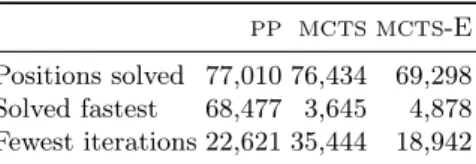
PNSwith the mobility initialization could not solve any position in less than 3 minutes in a preliminary set of about 50 positions. As a result we did not include this solver in our experiment with a larger set of positions. The experiments on y was carried out as follows. We generated 77,012 opening positions on a board of size 6. We then ranPPusing the reduction evaluation function,MCTS using playouts with a random policy, and a variant ofMCTSusing the same reduction evaluation instead of random playouts (MCTS-E). For each solver, we recorded the total number of positions solved within 60 seconds. Then, for each solving algorithm, we computed the number of positions among those 77,012 which were solved faster by this solver than by the two other solver, as well as the number of positions which needed fewer iterations of the algorithm to be solved. The results are presented in Table 3.
We see that the PP algorithms was able to solve the highest number of positions, 77,010 positions out of 77,012 could be solved within 60 seconds. We also note that for a very large proportion of positions (68,477),PPis the fastest algorithm. However,MCTSneeds fewer iterations than the other two algorithms on 35,444 positions. A possible interpretation of these results is that although iterations ofMCTS are a bit more informative than iterations ofPP, they take much longer. As a result,PPis better suited to situations where time is the most important constraint, whileMCTS is more appropriate when memory efficiency is a bottleneck. Note that if we discardMCTS-E results, then 72,830 positions are
Table 3. Number of positions solved by each algorithm and number of positions on which each algorithm was performing best.
PP MCTS MCTS-E Positions solved 77,010 76,434 69,298 Solved fastest 68,477 3,645 4,878 Fewest iterations 22,621 35,444 18,942
solved fastest byPP, 4180 positions are solved fastest byMCTS, 30,719 positions need fewest iterations to be solved byPP, and 46,291 need fewest iterations by
MCTS.
Figure 1 displays some of these results graphically. We sampled about 150 positions of various difficulty from the set of 77,012 y positions, and plotted the time needed to solve such positions by each algorithm against the time needed byPP. We see that positions that are easy forPPare likely to be easy for both
MCTS solvers, while positions hard for PPare likely to be hard for both other solvers as well. 0.1 1 10 0.1 1 10 Time PPtime PPtime MCTStime MCTS-E time
Fig. 1. Time needed to solve various opening positions in the game of y.
4.2 domineering
domineering is played on a rectangular board. The first player places a vertical 2 × 1 rectangle anywhere on the board. The second player places an horizontal 2 × 1 rectangle, and the games continues like that until a player has no legal moves. The first player that has no legal moves has lost.
domineering has already been studied in previous work by game search specialists as well as combinatorial game theorists [4, 16].2 While these papers focusing on domineering obtain solution for relatively large boards, we have kept ourselves to a naive implementation of both the game rules and the algo-rithms. In particular, we do not perform any symmetry detection nor make use of combinatorial game theory techniques such as decomposition into subgames. We presents results for the following algorithms: αβ, PNS with Transposi-tions (PNT) [27], PN2 [5], PP, PP with Transpositions (PPT) and PP2. The
PNSalgorithm could not find a single solution within 107 node expansion when transpositions where not detected and it is thus left out.
ForPNSvariants the standard mobility heuristic is used to compute the proof numbers and the disproof numbers at non solved leaves. ForPPvariants, we used the mobility heuristic as described in Section 3.2.
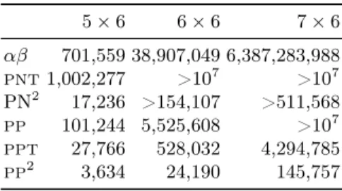
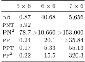
Tables 4 and 5 give the number of nodes and times for different algorithms solving domineering. αβ is enhanced with transposition tables, killer moves, the history heuristic and an evaluation function. We can see that on the smallest 5 × 6 board thatPPTgives the best results. On the larger 6 × 6 boardPPTis the best algorithm by far. On the largest 7 × 6 board, several algorithms run out of memory, and the best algorithm remainsPPT which outperforms both αβ and PN2.
Table 4. Number of node expansions needed to solve various sizes of domineering. 5 × 6 6 × 6 7 × 6 αβ 701,559 38,907,049 6,387,283,988 PNT 1,002,277 >107 >107 PN2 17,236 >154,107 >511,568 PP 101,244 5,525,608 >107 PPT 27,766 528,032 4,294,785 PP2 3,634 24,190 145,757
In their paper, Breuker et al, have shown that the use of transposition tables and symmetries increased significantly the performance of their αβ implemen-tation [4]. While, our proof-of-concept implemenimplemen-tation does not take advantage of symmetries, our results show that transpositions are of great importance in thePPparadigm as well.
2Some results can also be found on http://www.personeel.unimaas.nl/
Table 5. Time (s) needed to solve various sizes of domineering. 5 × 6 6 × 6 7 × 6 αβ 0.87 40.68 5,656 PNT 5.92 PN2 78.7 >10,660 >153,000 PP 0.24 20.1 >35.84 PPT 0.17 5.33 55.13 PP2 0.22 15.5 320.3 4.3 nogo
nogo is the misere version of the game of go. It was presented in the BIRS 2011 workshop on combinatorial game theory [8].3 The first player to capture
has lost.
We present results for the following algorithms: αβ,PNT[27], PN2 [5],
PP,
PPTandPP2. Again, the PNSalgorithm could not find a single solution within 107 node expansion and is left out.
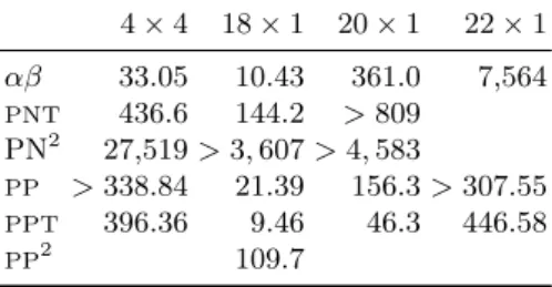
For standard board sizes such as 4 × 4 or 5 × 4, αβ gives the best results among the algorithms we study in this paper. We have noticed that for N × 1 boards for N ≥ 18,PPTbecomes competitive. Results for a few board sizes are given in Table 6 for the number of nodes and in Table 7 for the times.
Table 6. Number of node expansions needed to solve various sizes of nogo. 4 × 4 18 × 1 20 × 1 22 × 1 αβ 17,194,590 4,444,384 154,006,001 3,133,818,285 PNT 3,575,076 2,015,179 >107 >107 PN2 77,010 > 22, 679 > 29, 098 PP >107 864,951 6,173,393 >107 PPT 2,319,816 98,991 389,119 2,814,553 PP2 14,246
5
Conclusion
In this paper, we have presented how to use Product Propagation (PP) in order to solve abstract two-player games. We extendedPPso as to handle transposi-tions and to reduce memory consumption with the PP2 algorithm. For two of the games that have been tested (i.e., y, domineering), we found that our ex-tensions ofPPare able to better solve games than the other solving algorithms.
3
Table 7. Time (s) needed to solve various sizes of nogo. 4 × 4 18 × 1 20 × 1 22 × 1 αβ 33.05 10.43 361.0 7,564 PNT 436.6 144.2 > 809 PN2 27,519 > 3, 607 > 4, 583 PP > 338.84 21.39 156.3 > 307.55 PPT 396.36 9.46 46.3 446.58 PP2 109.7
For nogo,PPvariants outperformPNSvariants on all tested sizes, andPPdoes better than αβ on some sizes but αβ is better on standard sizes.
Being a best-first search algorithm,PPis quite related toPNSandMCTS, as such, it seems natural to try and adapt ideas that proved successful for these al-gorithms to the Product Propagation paradigm. For instance, whilePNSandPP
are originally designed for two-outcome games, future work could adapt the ideas underlying Multiple-OutcomePNS[22] to turnPPinto an algorithm addressing more general games. Adapting more elaborate schemes for transpositions could also prove interesting [18, 13, 23].
References
1. Louis Victor Allis, M. van der Meulen, and H. Jaap van den Herik. Proof-Number Search. Artificial Intelligence, 66(1):91–124, 1994.
2. Eric B. Baum and Warren D. Smith. Best play for imperfect players and game tree search. Technical report, NEC Research Institute, 1993.
3. Eric B. Baum and Warren D. Smith. A Bayesian approach to relevance in game playing. Artificial Intelligence, 97(1–2):195–242, 1997.
4. Dennis M. Breuker, Jos W.H.M. Uiterwijk, and H. Jaap van den Herik. Solving 8×8 domineering. Theoretical Computer Science, 230(1-2):195–206, 2000.
5. Dennis Michel Breuker. Memory versus Search in Games. PhD thesis, Universiteit Maastricht, 1998.
6. Cameron Browne, Edward Powley, Daniel Whitehouse, Simon Lucas, Peter Cowl-ing, Philipp Rohlfshagen, Stephen Tavener, Diego Perez, Spyridon Samothrakis, and Simon Colton. A survey of Monte Carlo tree search methods. Computational Intelligence and AI in Games, IEEE Transactions on, 4(1):1–43, March 2012. 7. Tristan Cazenave and Abdallah Saffidine. Score bounded Monte-Carlo tree search.
In H. van den Herik, Hiroyuki Iida, and Aske Plaat, editors, Computers and Games, volume 6515 of Lecture Notes in Computer Science, pages 93–104. Springer-Verlag, Berlin / Heidelberg, 2011.
8. C.-W. Chou, Olivier Teytaud, and Shi-Jin Yen. Revisiting Monte-Carlo tree search on a normal form game: Nogo. In Cecilia Chio, Stefano Cagnoni, Carlos Cotta, Marc Ebner, Anikó Ekárt, AnnaI. Esparcia-Alcázar, JuanJ. Merelo, Ferrante Neri, Mike Preuss, Hendrik Richter, Julian Togelius, and Georgios N. Yannakakis, edi-tors, Applications of Evolutionary Computation, volume 6624 of Lecture Notes in Computer Science, pages 73–82. Springer Berlin Heidelberg, 2011.
9. Timo Ewalds. Playing and solving Havannah. Master’s thesis, University of Al-berta, 2012.
10. Thomas Hauk, Michael Buro, and Jonathan Schaeffer. Rediscovering *-minimax search. In H. Jaap van den Herik, Yngvi Björnsson, and Nathan S. Netanyahu, editors, Computers and Games, volume 3846 of Lecture Notes in Computer Science, pages 35–50. Springer Berlin Heidelberg, 2006.
11. Helmut Horacek. Towards understanding conceptual differences between minimax-ing and product-propagation. In 14th European Conference on Artificial Intelli-gence (ECAI), pages 604–608, 2000.
12. Helmut Horacek and Hermann Kaindl. An analysis of decision quality of mini-maxing vs. product propagation. In Proceedings of the 2009 IEEE international conference on Systems, Man and Cybernetics, SMC’09, pages 2568–2574, Piscat-away, NJ, USA, 2009. IEEE Press.
13. Akihiro Kishimoto and Martin Müller. A solution to the GHI problem for depth-first proof-number search. Information Sciences, 175(4):296–314, 2005.
14. Akihiro Kishimoto, Mark H.M. Winands, Martin Müller, , and Jahn-Takeshi Saito. Game-tree search using proof numbers: The first twenty years. ICGA Journal, 35(3):131–156, 2012.
15. Levente Kocsis and Csaba Szepesvàri. Bandit based Monte-Carlo planning. In 17th European Conference on Machine Learning (ECML’06), volume 4212 of LNCS, pages 282–293. Springer, 2006.
16. Michael Lachmann, Cristopher Moore, and Ivan Rapaport. Who wins domineering on rectangular boards. volume 42, pages 307–315. Cambridge University Press, 2002.
17. Richard J. Lorentz. Amazons discover Monte-Carlo. In Computers and Games, Lecture Notes in Computer Science, pages 13–24. 2008.
18. Martin Müller. Proof-set search. In Computers and Games 2002, Lecture Notes in Computer Science, pages 88–107. Springer, 2003.
19. J.A.M. Nijssen and Mark H.M. Winands. An overview of search techniques in multi-player games. In Computer Games Workshop at ECAI 2012, pages 50–61, 2012.
20. Judea Pearl. On the nature of pathology in game searching. Artificial Intelligence, 20(4):427–453, 1983.
21. Stuart J. Russell and Peter Norvig. Artificial Intelligence — A Modern Approach. Pearson Education, third edition, 2010.
22. Abdallah Saffidine and Tristan Cazenave. Multiple-outcome proof number search. In Luc De Raedt, Christian Bessiere, Didier Dubois, Patrick Doherty, Paolo Fras-coni, Fredrik Heintz, and Peter Lucas, editors, 20th European Conference on Ar-tificial Intelligence (ECAI), volume 242 of Frontiers in ArAr-tificial Intelligence and Applications, pages 708–713, Montpellier, France, August 2012. IOS Press. 23. Abdallah Saffidine, Tristan Cazenave, and Jean Méhat. UCD: Upper Confidence
bound for rooted Directed acyclic graphs. Knowledge-Based Systems, 34:26–33, December 2011.
24. Abdallah Saffidine, Hilmar Finnsson, and Michael Buro. Alpha-beta pruning for games with simultaneous moves. In Jörg Hoffmann and Bart Selman, editors, 26th AAAI Conference on Artificial Intelligence (AAAI), pages 556–562, Toronto, Canada, July 2012. AAAI Press.
25. Maarten P.D. Schadd and Mark H.M. Winands. Best reply search for multiplayer games. IEEE Transactions Computational Intelligence and AI in Games, 3(1):57– 66, 2011.
26. Craige Schensted and Charles Titus. Mudcrack Y & Poly-Y. Neo Press, 1975. 27. Martin Schijf, L. Victor Allis, and Jos W.H.M. Uiterwijk. Proof-number search
and transpositions. ICCA Journal, 17(2):63–74, 1994.
28. James R. Slagle and Philip Bursky. Experiments with a multipurpose, theorem-proving heuristic program. Journal of the ACM, 15(1):85–99, 1968.
29. David Stern, Ralf Herbrich, and Thore Graepel. Learning to solve game trees. In 24th international conference on Machine learning, ICML ’07, pages 839–846, New York, NY, USA, 2007. ACM.
30. Nathan R. Sturtevant. A comparison of algorithms for multi-player games. In Computer and Games, 2002.
31. H. Jaap van den Herik and Mark H.M. Winands. Proof-Number Search and its variants. Oppositional Concepts in Computational Intelligence, pages 91–118, 2008. 32. Jack van Rijswijck. Search and evaluation in Hex. Technical report, University of
Alberta, 2002.
33. Mark H.M. Winands, Yngvi Björnsson, and Jahn-Takeshi Saito. Monte Carlo tree search in lines of action. IEEE Transactions on Computational Intelligence and AI in Games, 2(4):239–250, 2010.
34. Mark H.M. Winands, Yngvi Björnsson, and Jahn-Takeshi Saito. Monte-Carlo tree search solver. In H. Jaap van den Herik, Xinhe Xu, Zongmin Ma, and Mark H.M. Winands, editors, Computers and Games, volume 5131 of Lecture Notes in Com-puter Science, pages 25–36. Springer, Berlin / Heidelberg, 2008.