JĘDRZEJ BIAŁKOWSKI is a Senior Lecturer in the Department of Economics and Finance, University of canterbury, christchurch, New Zealand. Email: jedrzej. [email protected] SERGE DAROLLES is an Adjunct Professor at the Université Paris Dauphine, DRM Finance and center for Research in Economics and Statistics (cREST), France. Email: [email protected] GAËLLE LE FOL is Professor of Finance at the Université Paris Dauphine, DRM Finance and center for Research in Economics and Statistics (cREST), France. Email: [email protected]
Keywords: intra-day trading volume, VWAP orders, execution risk, trading costs in securities markets.
This paper proposes a new dynamic approach to modelling intra-day trading volume based
on factor models. It assumes that intra-day volume can be decomposed into two parts each
predicted using separate time-series models. By enabling more accurate prediction of intra-day
volume, this methodology allows for a significant reduction in the cost of executing Volume
Weighted average Price orders.
1rEdUCInG ThE rISK oF VWAP
ordErS EXECUTIon —
A nEW
APProACh To modEllInG
InTrA-dAY VolUmE
In an era of increasing competition in financial services, financial institutions are spending more resources on broadening the array and reducing the price of products offered to clients. This also applies to broking houses, which have a vital interest in reducing costs associated with the execution of their clients’ orders.
This paper presents a technique that aims to reduce the execution risk of VWAP (Volume Weighted Average Price) orders, which are orders to buy or sell a certain amount of a stock during the specified period at the VWAP. VWAP is calculated by dividing the value of trades by the volume over a specified period.
To illustrate the issue, very simply, suppose that trading takes place at only three times (t1, t2, and t3) during the day, with 20 per cent of the trading volume expected to occur at t1, 50 per cent at t2, and 30 per cent at t3. An investor wishing to purchase 100,000 shares using a VWAP order would place orders for 20,000 to be bought at t1, 50,000 at t2, and 30,000 at t3. If the market trading volume matched expectations, the average purchase price for the investor would match the VWAP of trades undertaken on the market during the day. however, the pattern of trading during the day may differ from that expected, because the volume profile is not stable, thus leading to deviations in the average purchase price from the VWAP benchmark (Gefen and Jones 2011). As Mcculloch and Kazakov (2010) note, ‘a riskless VWAP trading strategy is not possible without knowledge of final market volume’. We propose a dynamic titled VWAP strategy that alleviates these problems by adding some short-term, stock-specific, trading dynamics to the historical, market-wide, daily trading pattern.
Algorithm trading is estimated to be responsible for 73 per cent of institutional equity trading in the United States, and VWAP execution orders are a significant part of it (see, for example, Mackenzie 2009, chlistalla 2011, and Nybo 2011). There are at least two reasons why this type of order has become so popular. First, by selecting this type of order, large investors hope to reduce the market impact of their trades (i.e. the change in a stock’s price due to the execution of the trade) which is one of the factors affecting the total cost of the trade. (Institutional investors can expect a negative price reaction to a large sell order and a positive price reaction to a large buy order, with such market impacts reducing the profit of the trade.) Second, VWAP orders allow foreign investors to reduce the risk of placing orders before the opening of the market that are to be executed at the opening price or via some limit order. The VWAP order generates an average trade price which is close (if the VWAP algorithm works well) to the average price at which all transactions in the market are completed that day, thereby avoiding possible execution of the order at an extreme price. While VWAP orders seem to be a
remedy for a number of investors’ problems, a word of caution is required. Recent studies by Gefen and Jones (2011) and Quantitative Service Group LLc (2009) have shown that the application of so-called naive algorithms for VWAP execution can lead to an increase in execution risk.
Modelling intra-day trading volume
One of the distinctive attributes of intra-day trading volume is its higher level at the beginning and the end of a trading day. This feature is known as the U-shape of intra-day volume. The U-shape for the US market was reported by Admati and Pfleiderer (1988), Jain and Joh (1988), Foster and Viswanathan, (1990), chan et al. (1995) and others. For French and Japanese markets, U-shaped volume was confirmed by the studies of Gouriéroux et al. (1999) and Konishi (2002), respectively. For the Australian market, Aitken et al. (1994) reported that the U-shape is observed for the number of transactions during a trading day. Kalev et al. (2004) reported the U-shape for traded volume for the companies with the highest frequency of trading. Several explanations of this phenomenon can be found. The most important are: the accumulation of information during non-trading hours; the concentration of trades; the opening of other key stock markets; and the low activity of traders during lunchtime.
The modelling of intra-day volume is of vital interest to a trader who is responsible for executing clients’ VWAP orders. If a trader’s aim is only to sell or buy a stock at VWAP, the only knowledge which he or she needs is the U-shape of the volume for a particular day. By analysing an area below the U-curve, a trader is able to determine what percentage of the order needs to be executed in each part of the day. It is worth highlighting, that what he or she really needs is the intra-day shape, not the level, of the volume.
The standard method of predicting the U-shape of the volume for a given stock has been to use an average of trading patterns over a certain number of preceding days (at either a market-wide or individual stock level). Each day is divided into a constant number of time intervals (buckets) and the average volume is calculated separately for each bucket. The details of this approach are described by Madhavan (2002) and Manchaladore et al. (2010).
This model is known as the classical or static approach. If volume U-shape remains unchanged over time, it would be unquestionably a very good model. Unfortunately, the daily dynamics of the volume are more complex. consequently, more advanced models for the U-shape of intra-day volume need to be introduced. Moreover, the static approach means that the volume structure is only updated gradually as the historical average changes, rather than being updated dynamically in response to recent information.
In this paper, we propose a new dynamic approach based on factor models (see also Bialkowski et al. 2008). It assumes that intra-day volume can be decomposed into two parts each predicted using separate time-series models. The first describes intra-day trading volume patterns for the whole exchange, and changes in that pattern over time resulting in changes in the first component of the intra-day volume for individual stocks. For obvious reasons, we will call it the market component. The second component depicts the intra-day dynamics of the volume, which is distinctive for each examined stock. For example, if the company announces a significant earnings increase or decrease, the second component of the volume decomposition is expected to grow.
The turnover ratio was selected as the measure of volume. It is defined as:
it it
it
V
N
x =
wherexit denotes the turnover series for stock i at the intra-day time t, Vit is the number of shares traded at time t, Nit is the number of shares on issue at time t. The total number of stocks under scrutiny is K. In case of decomposition of turnover into the market and its specific
The VWaP order generates an average trade
price which is close (if the VWaP algorithm
works well) to the average price at which all
transactions in the market are completed that
day, thereby avoiding possible execution of the
order at an extreme price.
parts, the parameter K should be equal to the number of stocks in a main index.
In order to complete the factor decomposition, we apply Principal component Analysis (PcA).2 For each stock
included in the index (40 in the specific case studied here, see below) we prepare a time series dataset consisting of 20-minute intervals (bucket) for each trading day for the past three months. Since each day is thus divided into 25 buckets and with approximately 21 trading days per month, each time series has approximately 1575 observations. For each day, we apply PcA analysis to the 40 times series of intra-day trading volume over the past three months. It allows for the following decomposition of volume:
t
i
t
i
t
i
c
y
x
,
=
,
+
,
(1)where the common or market component of turnover denoted as cit is the derived first principal component and the specific part of turnover yit is the remainder. One of the methods of evaluating the validity of the PcA decomposition is analysis of variance explained by each of the components. According to our results for the French stock market, the market component of such decomposition is able to explain, on average, 40 per cent of the observed variance in intra-day volume. Therefore, it is suitable to describe the volume changes caused by the movements of the whole market.
As was mentioned earlier, the decomposition is the first part of the analysis. The next step is to construct separate models for the market component and the specific component of the turnover.
The market component is expected to capture overall (market-wide) intra-day turnover fluctuation, i.e. the daily U-shape, and we refer to this as the seasonal component. To predict this component we propose a model which is often used by traders to predict the total volume. It is based on the idea that the U-shape for the next day’s volume can be predicted by the historical arithmetical average over the past L-trading days. Undoubtedly, the advantage of this static approach is its simplicity. however, the serious drawback of this approach is that it ignores the intra-day, stock-specific, dynamics of turnover. Note that, if we apply this method to the market component obtained from the principal component decomposition, we do not face this problem.
hence,
c
i,trepresents the market historical average of intra-day volume for time bucket t over the past L-trading days until day j in the examined sample. It is given by:c
i,t, j= 1
L
c
i,tj−l l=1 L∑
(2)l
j
j
t
i
c
,
,
is the market component of turnover for stock i atthe intra-day time t on the j-l day of the examined sample. The specific component (i.e. the volume not explained by the first (market) principal component for each stock) is modelled by using either an ARMA model or a self-exciting threshold autoregressive (SETAR) model. The ARMA (1, 1) with white noise is defined as:
t
i
t
i
t
i
y
y
,
1
,
1
2
,
(3)
The alternative model is SETAR defined as:
.
,
1 , , 22 1 , 21 1 , , 12 1 , 11 ,
t i t i t i t i t i t i t iy
y
y
y
y
(4)The application of the SETAR model gives further insight into the dynamics of the specific components of turnover. The construction of the model is based on the idea that the dynamics of the specific component of turnover are different when the specific component of turnover has a value higher than the estimated threshold. Parameters of the SETAR model are estimated by using the sequential conditional least squares method. A detailed description of the estimation technique can be found in Frances and van Dijk (2000). This particular choice of model for the specific part of volume is based on analysis of autocorrelation and partial autocorrelation functions. In the selection process we seek a model that is as simple as possible with goodness of fit superior to the static approach.
Implementation of the model to trading
Each day, traders responsible for the execution of VWAP orders have to decide between two alternatives. The first one is to predetermine the trading strategy at the beginning of a session and then follow it until the end ofeach day, traders responsible for the execution of VWaP orders have to
decide between two alternatives. The first one is to predetermine the trading
strategy at the beginning of a session and then follow it until the end of the
validity of the order. The second assumes updating the execution strategy
during the day. Our results show that the second option, with the application
of the seTaR or aRMa model, leads to a reduction in execution risk.
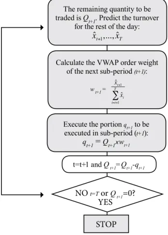
the validity of the order. The second assumes updating the execution strategy during the day. Our results show that the second option, with the application of the SETAR or ARMA model, leads to a reduction in execution risk. This section briefly describes the ‘updating the execution’ strategy by incorporating new information available from the market. Figure 1 presents the scheme of the algorithm. First, we predict the turnover for the entire day by using the SETAR or ARMA model applied to itsspecific part and the static approach applied to the market component. We obtain 25 (number of 20-minute intervals during one trading day) predictions of trading volumes (
x
ˆ
1,...,
x
ˆ
25). The proportion of the order to execute at the beginningof the day (the first time interval) is equal to:
25 1 1ˆ
ˆ
i ix
x
.At the end of the first period, we observe x1 and use it to predict new (
x
ˆ
2,...,
x
ˆ
25). The proportion of the remaining volume to execute in the second period is then equal to
25 2 2ˆ
ˆ
i ix
x
.The procedure is continued until the end of the day. As a consequence, at the very beginning of the day, the trader using the above strategy will trade without information about that day. Then, with time passing,
he or she will improve predictions and be able to beat a trader who predicted the whole U-shaped volume at the beginning of the trading day. Further details of the approach are available in Bialkowski et al. (2008).
Data
To illustrate the approach, we use a dataset from the European stock market. Our examination focuses on all stocks included in the cAc40 index at the beginning of September 2004. The analysis is based on a sample ranging from September 2003 to the end of August 2004. The tick-by-tick volume and prices were obtained from the EURONEXT database. The data is aggregated to 20-minute intervals. The 20-minute volume is defined as the sum of the traded volumes while a 20-minute price is identified by taking an arithmetic average over 20-minute periods. We have restricted the examination to continuous trading between 9.20 am and 5.20 pm.3 Finally, as a proxy
of volume, we chose the turnover defined as the traded volume divided by the outstanding number of shares for a particular stock. Our selection is consistent with a few previous studies on volume (see, for example, Lo and Wang 2000). For the sake of brevity, we have presented the results for six out of 40 companies. The other results are available on request.
Results
First, we examine how well our statistical models fit the data, and then consider how well VWAP trading strategies based upon them perform, using the size of deviations of achieved average prices from actual VWAP as a performance measure.
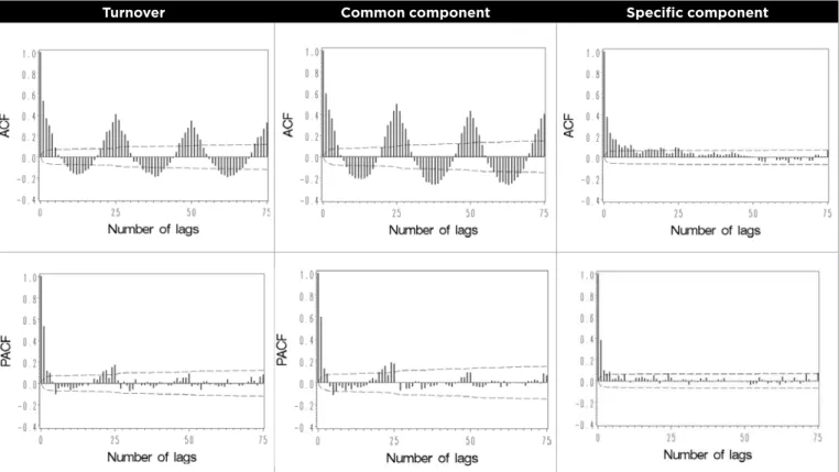
Figure 2 presents plots of autocorrelation and partial autocorrelation functions (AcF and PAcF) of the turnover of France Telecom stock. It presents the results for three trading days, equivalent to 75 buckets (1 bucket is 20 min). The left graphs show typical characteristics of the intra-day turnover, namely cyclical fluctuations. From the middle graphs, one recognises the ability of the common
component to capture cyclical variations. The final graphs illustrate AcF and PAcF for the specific part of turnover. The fast decay of the autocorrelation suggests that the ARMA-type model is suitable for depicting this time series. For next day’s prediction of the cyclical fluctuations of the daily U-shape, the historical average of the first component of PcA decomposition is used. The dynamic part of the daily U-shape, defined as a specific component after PcA decomposition, is modelled by a SETAR or ARMA model.4 The application of those models is feasible
only because the specific component of intra-day volume is a stationary time series.
All companies from the cAc 40 index were analysed in order to determine whether the approach presented above can reduce the risk of execution of VWAP orders. Given the space constraints, we report the results for six companies characterised by high capitalisation.
FIGURE 1: Scheme of the dynamic VWAP order execution algorithm
t=t+1 and Q
t+1=Q
t+1-q
t+1Execute the portion
qt+1to be
executed in sub-period (
t+1):
q
t+1=
Q
t+1xw
t+1Calculate the VWAP order weight
of the next sub-period
(t+1):
w t+1 = ˆxt+1 ˆxi i=t+1
T
∑
The remaining quantity to be
traded is Q
t+1. Predict the turnover
for the rest of the day:
ˆx
t+1,..., ˆx
TNO
t=Tor
Q
t+1=0?
YES
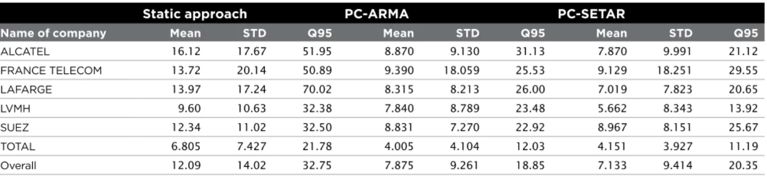
Table 1 reports the basic statistics of turnovers. The highest average 20-minute turnover is observed for Alcatel. It is equal to 0.04 per cent and the lowest turnover is observed for LVMh. The turnover in the 20-minute time bucket with the highest turnover (indicated by the Q95 quantile) was 2.5 times the average turnover of all of the time buckets. In Table 2, we report the average cost (for deviations of price achieved from the actual VWAP) of executing VWAP orders for the period between 3 September and 2 December 2003. The reported results are based on the pre-determined strategy. Three models for intra-day volume are examined. Two are the models developed above, one using the ARMA approach (Pc-ARMA) for the specific component and the other using the SETAR approach (Pc-SETAR). The third is based on a static approach to predicting the daily dynamics of volume which assumes that the volume during a particular time interval can be approximated by taking the historical average. Table 2 was prepared in the following way: for each day of the three-month period examined, actual VWAP is compared with that predicted by each of the models. The mean absolute percentage error (MAPE) is used as an error measure.
The reported results confirm the effectiveness of the proposed factor decomposition models. The application of a Pc-ARMA model allows for the reduction of the average cost of VWAP orders by more than 4 basis points (bps) in comparison with the static approach. In turn, selection of Pc-SETAR provides the opportunity for a
further 1 bp decrease in comparison with Pc-ARMA. The superiority of Pc models is also confirmed by the results of the 95 per cent quantile comparison. The 95 per cent quantiles indicate the average MAPE for the 5 per cent of days in which the strategy performed worst. On average, the 95 per cent quantile is two times lower for Pc models than for the static approach. The best results are obtained for LAFARGE with reductions of 44 bps and 49 bps for Pc-ARMA and Pc-SETAR, respectively. In order to give the reader a better understanding, we randomly selected two succeeding days from our sample to prepare Figure 3. This allows us to evaluate the goodness of fit for those two successive days in November 2003. The left graphs show the daily U-shape of intra-day turnover and its prediction for France Telecom stock. In turn, the middle graphs present a prediction of the seasonal part of the daily U-shape, as an historical average of the common component. It is the same shape across all examined stocks. The right graphs in Figure 3 illustrate the dynamic part of daily U-shapes for both stocks. It is clear that differences in the U-shape are due to specific components. It is worth highlighting also that there is no coincidence in the strong similarity between average common components for the two successive days in November 2003. To sum up, through the application of the proposed models, a trader is able to reduce the cost of VWAP orders and, moreover, his or her chance of large costs measured by the 95 per cent quantile is lower. Therefore, VWAP trade orders can be offered at a lower commission fee to clients.
FIGURE 2: Autocorrelation and partial autocorrelation functions of the turnover and the two components for France Telecom stock
Turnover Common component Specific component
note: The left graphs show typical characteristics of the intra-day turnover, namely seasonal variations. From the middle graphs, one recognises the ability of a common component to capture seasonal variations. The final graphs illustrate ACF and PACF for the specific part of turnover. The fast decay of the autocorrelation suggests that the ArmA-type model is suitable to depict this time series. The graphs present 75 lags equivalent to three trading days.
TABLE 1: Summary statistics for the intra-day aggregated turnover over 20-minute intervals, for the period between 2 September 2003 and 31 August 2004
Name of company Mean STD Q5 Q95
ALcATEL 0.0381 0.0383 0.0062 0.1064 FRANcE TELEcOM 0.0123 0.0115 0.0025 0.0312 LAFARGE 0.0188 0.0307 0.0035 0.0477 LVMh 0.0105 0.0185 0.0018 0.0276 SUEZ 0.0162 0.0182 0.0032 0.0418 TOTAL 0.0150 0.0277 0.0031 0.0373 Overall 0.0185 0.0241 0.0034 0.0487
note: The table reports basic statistics for the turnover ratio selected as measure of volume. The ratio is defined as: number of shares traded at each 20-minute bucket divided by the number of shares on issue on a given trading day. STd, Q5, and Q95 are standard deviation, 5% quantile and 95% quantile, respectively.
TABLE 2: Summary statistics for cost of execution VWAP orders for the period between 3 September and 2 December 2003
Static approach PC-ARMA PC-SETAR
Name of company Mean STD Q95 Mean STD Q95 Mean STD Q95
ALcATEL 16.12 17.67 51.95 8.870 9.130 31.13 7.870 9.991 21.12 FRANcE TELEcOM 13.72 20.14 50.89 9.390 18.059 25.53 9.129 18.251 29.55 LAFARGE 13.97 17.24 70.02 8.315 8.213 26.00 7.019 7.823 20.65 LVMh 9.60 10.63 32.38 7.840 8.789 23.48 5.662 8.343 13.92 SUEZ 12.34 11.02 32.50 8.831 7.270 22.92 8.967 8.151 25.67 TOTAL 6.805 7.427 21.78 4.005 4.104 12.03 4.151 3.927 11.19 Overall 12.09 14.02 32.75 7.875 9.261 18.85 7.133 9.414 20.35
FIGURE 3: Application of PC-SETAR model to prediction of daily U-shape for two successive days in November 2003
Name of
company Turnover Average common component Estimated specific component
Fr an ce T el ec o m Fr an ce T el ec o m
note: The observed volumes on 18 and 19 november are denoted by the solid line. The dashed line line denotes the forecast of the U-shape. The upper panel refers to 18 november and the lower panel to 19 november 2003. The left graphs show daily U-shape of intra-day turnover (solid line) and its prediction (dashed line) for France Telecom. The middle graphs present predictions of the cyclical part of daily U-shape, and, as the historical average of the common component, it is very similar for the two successive days. The right graphs illustrate the dynamic part of the daily U-shape for the two days.
Through the application of the proposed models, a trader is able to reduce
the cost of VWaP orders and, moreover, his or her chance of large costs
measured by the 95 per cent quantile is lower. Therefore, VWaP trade
orders can be offered at a lower commission fee to clients.
conclusion
In this paper, we have presented a methodology for modelling intra-day volume. It is based on decomposing a single stock’s trading volume into a market and a specific component. The first part, describing market volume behaviour, is modelled by an historical average.
The specific part, volume, is described using well-known econometrics models such as ARMA and SETAR. The application of the discussed methodology can enable more accurate prediction of intra-day volume. As a consequence, based on the empirical estimates, a trader making use of the proposed model would be able to reduce significantly the cost of executing VWAP orders.■
References:
Admati, A. and Pfleiderer, P. 1988, ‘A theory of intraday patterns: volume and price variability’, Review of Financial Studies, vol. 1, pp. 3–40.
Aitken, M., Brown, P. and Walker, T. 1994, ‘Intraday patterns in returns, volume, volatility and trading frequency on SEATS’, working paper, University of Sydney.
Biais, B., hillion, P. and Spatt, c. 1995, ‘An empirical analysis of the limit order book and the order flow in the Paris Bourse’, Journal of Finance, vol. 50, pp. 1655–89.
Bialkowski, J., Darolles S. and Le Fol, G. 2008, ‘Improving VWAP strategies: a dynamic volume approach’, Journal of Banking and
Finance, vol. 32, pp. 1709–22.
chan, K.c., christie, W.G. and Schultz, P.h. 1995, ‘Market structure and the intraday pattern of bid/ask spreads for NASDAQ securities’,
Journal of Business, vol. 68, pp. 35–60.
chlistalla M. 2011, ‘high-frequency trading: better than its reputation?’, Deutsche Bank Research, 7 February.
Foster, D., and Viswanathan, S. 1990, ‘A theory of intraday variation in volume, variance and trading costs in securities market’, Review of
Financial Studies, vol. 3, pp. 593–624.
Frances, P. and van Dijk, D. 2000, Non-linear time series models in
empirical finance, cambridge University Press.
Gefen, O. and Jones, J. 2011, ‘Exploding the myth of ‘safe’ VWAP: understanding the risks of a VWAP algorithmic strategy’, Investment Technology Group, June.
Gouriéroux, c., Jasiak, J. and Le Fol, G. 1999, ‘Intra-day market activity’, Journal of Financial Markets, vol. 2, pp. 193–226.
Jain, P.c. and Joh, G. 1988, ‘The dependence between hourly prices and trading volume’, Journal of Financial Quantitative Analysis, vol. 23, pp. 269–83.
Kalev, P.S, Liu, W., Pham, P.K. and Jarnecic, E. 2004, ‘Public information arrival and volatility of intraday stock returns’, Journal of
Banking and Finance, vol. 28, pp. 1441–67.
Konishi, h. 2002, ‘Optimal slice of a VWAP trade’, Journal of Financial
Markets, vol. 5, pp. 197–221.
Lo, A. and Wang, J. 2000, ‘Trading volume: definition, data analysis, and implication of portfolio theory’, Review of Financial Studies, vol. 13, pp. 257–300.
Mackenzie, M. 2009, ‘high frequency trading under scrutiny,’ Financial
Times, 28 July.
Madhavan, A. 2002, ‘VWAP strategies transaction performance: the changing face of trading investment guides series’, Institutional Investor Inc., pp. 32–8.
Manchaladore, J., Palit, I. and Soloviev, O. 2010, ‘Wavelet
decomposition for intra-day volume dynamics’, Quantitative Finance, vol. 10, iss. 8, pp. 917–30.
Mcculloch, J. and Kazakov, V. 2010, Mean variance optimal VWAP
trading. Available at http://ssrn.com/abstract=1803858
Nybo, A. 2010, ‘TABB group sees low-touch order channels
accounting for 62% of buyside firms’ options trading by 2011’, Business Wire, 26 July.
Quantitative Service Group LLc Analyst Team 2009, ‘Beware of the VWAP trap’, research note, November.
k t k t t i k k t t t i i t i x Cov x C C Covx C C x 1 ( , ) 1 ( ,, ) 1 1 1 , 1 ,
Notes
1. Acknowledgements: The authors are most grateful to the Managing Editor Kevin Davis for very helpful comments and suggestions that significantly improved this paper. Serge Darolles and Gaëlle Le Fol gratefully acknowledge financial support of the chair QUANTVALLEY/Risk Foundation: Quantitative Management Initiative (QMI). Jędrzej Białkowski is grateful to BNZ bank for funding support, but none of the views expressed in this paper should be attributed to them.
2. The first step of the procedure is calculating K K the dimension variance-covariance matrix. The spectral decomposition of this matrix leads to K orthogonal vectors,Ctk xit'uk
= , with T-dimension each. uk is kth eigenvector. Each eigenvector is associated with a positive eigenvalue λk such that:Cov(Ctk,Ctl)=lkdkl, where
δkl is Krononecker symbol. After simplification, we obtain the decomposition in the form given by the formula:
Thus, the turnover for stock i at time t is given by:
t i t i t i
c
y
x
,=
,+
,1 1 , 1 ,t i 1 ( it, t) t i x Cov x C C c l + =
, first principal component,
k t k k t t i k t i Covx C C y 1 ( , ) 1 , ,
, other principal components.
3. Note that we use all the intra-day observations from 9.00 am to 9.20 am to get the 9.20 observation and so on for each time bucket until the 5.20 pm observation.
4. These models are called Pc-ARMA and Pc-SETAR hereafter.
k t k k t t i k t i Cov x C C y 1 ( , ) 1 , ,