Sequential Halving Applied to Trees

Sequential Halving applied to Trees

Tristan Cazenave

Abstract—Monte Carlo Tree Search (MCTS) is state of the art for multiple games and problems. The base algorithm

currently used for Monte Carlo Tree Search is UCT. We propose an alternative Monte Carlo Tree Search algorithm: Sequential Halving applied to Trees (SHOT). It has multiple advantages over UCT: it spends less time in the tree, it uses less memory, it is parameter free, at equal time settings it beats UCT for a complex combinatorial game and it can be efficiently parallelized.

Index Terms—Monte Carlo Tree Search, Sequential Halving, SHOT, UCT, Nogo.

✦

1

I

Monte Carlo Tree Search [7] has been very suc-cessful in a number of games and single agent problems [3], [4] such as Go [7], General Game Playing [9], [12] and Morpion Solitaire [13]. The standard Monte Carlo Tree Search algorithm is UCT [11]. It uses the UCB bandit formula [2]. Alternative algorithms have been designed for bandits. For example Sequential Halving [10] allocates multiple playouts to each move. It runs a few rounds and it is given in advance the number of playouts it will use. We propose to adapt Sequential Halving to Monte Carlo Tree Search and to name the resulting algorithm SHOT.

There is a number of reasons why SHOT is worth considering:

• SHOT spends less time in the tree than UCT. • SHOT uses less memory than UCT.

• At equal time settings SHOT beats UCT for a typical combinatorial game.

• It can be parallelized efficiently. • There is no need to tune a parameter.

SHOT differs significantly from the tradi-tional UCT-like model of MCTS, as it does not execute the usual selection-expansion-simulation-backpropagation loop. Instead it allocates a budget of playouts to each move, this is why it spends less time in the tree and can be parallelized efficiently. • T. Cazenave is at LAMSADE, Universit´e Paris-Dauphine, 75016

Paris, France.

email: cazenave@lamsade.dauphine.fr

SHOT does the opposite of usual pruning heuris-tics for MCTS. Progressive widening [8] and pro-gressive unpruning [5] start with only the most promising moves and then extend the number of moves under consideration at a node when the number of playouts increase. On the contrary SHOT starts with all the possible moves and gradually decreases the number of moves under consideration. SHOT does not use domain dependent knowledge to prune the moves.

SHOT is parameter free as is Nested Monte Carlo Search (NMCS) [4]. However SHOT develops a tree near the root and performs simple playouts outside of this tree whereas NMCS does search all along the game with nested playouts, also searching near the end of the game.

SHOT can be applied to single-player, two-player and multi-player games. In this paper it is applied to a two-player game.

The second section is about Sequential Halving, the third section deals with SHOT, the fourth section details experiments, the last section concludes.

2

S

H

Sequential Halving [10] is an algorithm that is based on sequential elimination of moves. The algorithm proceeds in rounds. In each round the remaining moves are sampled uniformly. The number of play-outs is fixed at the start of the algorithm. Parts of the budget of playouts are allocated independently to moves during the few sequential rounds. A round consists of playing a fixed number of playouts for each remaining move. After each round the number

of moves under consideration is divided by two. Only the best half of the moves with the largest empirical averages are kept for the next round. When there is only one move left, the algorithm stops and sends back the move.

The number of playouts allocated to a move in each round is given by the following formula:

j _budget

|S|×⌈log2(|possibleM oves|)⌉

k

where budget is the total number of playouts that the algorithm will use, S is the set of remaining moves and possibleM oves is the set of all possible moves.

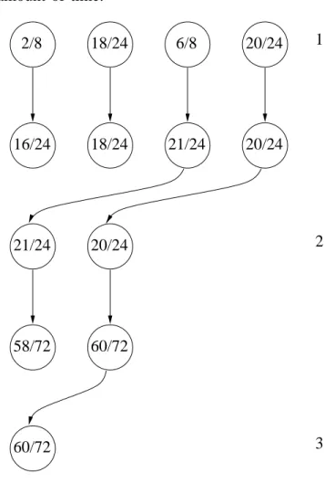
Figure 1 gives an example of Sequential Halving applied to a position with four moves and a budget of sixty-four playouts. At the beginning of the algorithm, all four moves have zero wins and zero playouts. Then the algorithm decides to try each move eight times since there are four possible moves and the budget is sixty-four (j_4×⌈log64

2(4)⌉

k

= 8). So

after the first round the four possible moves have empirical averages of 2/8, 8/8, 6/8 and 7/8. The two best moves (i.e. the moves that have the 8/8 and 7/8 empirical averages) are selected for the next round. Then the algorithm allocates j_2×⌈log64

2(4)⌉

k

= 16

playouts to each of these two remaining moves for the second round. After the second round, the resulting empirical averages are 18/24 and 20/24 so the best move that has the 20/24 empirical average is selected and as it is the only remaining move it is returned as the best move by the algorithm.

Sequential Halving has interesting theoretical properties. Instead of minimizing the regret as in UCB [2], Sequential Halving maximizes the proba-bility of choosing the best arm having the maximal expected reward. In [10], they prove a bound on the probability to erroneously eliminate the best arm. If

n is the number of arms, the multiplicative gap from

the lower bound on the number of required arm pulls to reach a given probability is in log log n while in previous algorithms the gap was in log n. The exact theorem is: for succeeding with probability at least 1 − δ, the algorithm needs a total of at

most T = O(H2 × log(n) × log(log(n)_δ )) arm pulls. Where H2 = maxi6=1(_∆i2

i) and ∆i = p1 − pi and

p1 ≥ p2 ≥ ... ≥ pn are the expected rewards of the arms.

These results were established using previous work on complexity measure [1].

Sequential Halving scales better than other algo-rithms when the number of possible moves grows

[10]. The paper on Sequential Halving also ad-dresses the fixed confidence setting in which the number of arm pulls is not fixed but the error probability is fixed.

Sequential Halving is given in algorithm 1.

6/8 7/8 0/0 0/0 0/0 0/0 20/24 8/8 7/8 2/8 20/24 8/8 18/24 1 2 3

Fig. 1. Sequential Halving for four possible moves and a budget of sixty-four playouts

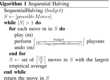
Algorithm 1 Sequential Halving

SequentialHalving (budget)

S ← [possibleM oves]

while |S| > 1 do

for each move m in S do

play (m)

perform j_|S|×⌈log budget

2(|possibleM oves|)⌉

k

playouts undo (m)

end for

S ← set of l|S|₂ m moves in S with the largest empirical average

end while

3

S

H

A

T

Sequential Halving is adapted when there is a fixed budget. When we use Sequential Halving in com-bination with tree search, we may come back to an already visited node with an increased budget. The policy that SHOT uses in this case is to consider the already allocated budget and the new budget as a whole. The overall budget is distributed as if it was given at first. The information on the node such as the number of playouts and the number of wins for each move are stored in the transposition table entry. This information is used to allocate the new budget so as not to give to a move more playouts than what it would have been given if the allocated budget and the new budget were considered as a whole. So the algorithm looks in the transposition table entry at the number of playouts that have already been given to the move and gives it the difference between the new budget for the move and the number of playouts already given.

An example of the behaviour of SHOT coming back to a previously explored node is given in figure 2. During the previous exploration of the node the four possible moves have been explored using Sequential Halving with a budget of sixty-four playouts. It resulted in empirical averages of 2/8, 18/24, 6/8 and 20/24 for the four possible moves. Now, SHOT comes back to the node with a budget of one hundred and twenty-eight playouts. It considers the overall budget as the sum of the budget previously spent at the node and of the budget still to be spent. The overall budget is 64 + 128 = 192.

It then calculates the budget to be allocated to each move in the first round using the formula

j _{t.budgetN ode+budget}

|S|×⌈log2(|possibleM oves|)⌉

k

where t.budgetNode is the budget already spent at the node during previous calls (64), budget is the budget to spend during the current call (128), and S is the set of remaining moves which is the set of all possible moves since it is the first round. So each possible move is allocated j_4×⌈log64+128

2(4)⌉

k

= 24 playouts. However each

move has already used some playouts the last times the node has been visited. So SHOT only gives each move the difference between the number of allocated playouts and the already used playouts. It gives sixteen playouts to the first move that has 2/8 and to the third move that has 6/8, and no playout to the other two moves that already have used

twenty-Algorithm 2 Sequential Halving applied to Trees

SHOT (board, budget, budgetU sed, playouts,

wins)

S ← possible moves

if board is terminal then

update playouts, wins and return

end if

if budget= 1 then

result← playout(board)

update playouts, budgetU sed, wins and return

end if

if |S| = 1 then

u← 0, p ← 0, w ← 0

SHOT (play(board, move), budget, u, p, w)

update playouts, budgetU sed and wins return move

end if

t← entry in the transposition table

if t.budgetN ode≤ |S| then

for move m in S with zero playouts do

result← playout(play(board, m))

update playouts, budgetU sed, wins and t return if budget playouts have been played

end for end if

sort moves in S according to their mean

b← 0

while |S| > 1 do

b← b + max(1,j_|S|×⌈logt.budgetN ode+budget

2(|possibleM oves|)⌉

k

)

for move m in S by decreasing mean do if t.playouts[m] < b then

b1 ← b − t.playouts[m]

if at root and |S| = 2 and m is the first

move in S then

b1 ← budget − budgetU sed − (b − t.playouts[secondM ove])

end if

b1 ← min(b1, budget − budgetU sed) u← 0, p ← 0, w ← 0

SHOT (play(board, m), b1, u, p, w)

update playouts, budgetU sed, wins and t

end if

break if budgetU sed≥ budget

end for

S ← sort l|S|₂ m best moves in S break if budgetU sed≥ budget

end while

update t.budgetN ode return first move of S

four playouts. After this first round we have the four moves that each have 24 playouts and empirical averages of 16/24, 18/24, 21/24 and 20/24. The best two moves are selected for the second round. This time they are allocated j_2×⌈log64+128

2(4)⌉

k

= 48 more

playouts using the same formula as for the first round. After the playouts have been played it results in empirical averages of 58/72 and 60/72. The best move is selected and the algorithm sends it back.

Due to the multiple visits of a node it happens that the budget allocated to a node is not completely used. In this case it is saved and reallocated to the best move at the root during the last round. It helps verifying the best move really has a better empirical average than the second best move. However other reallocation strategies can be thought of.

In order to avoid waste of memory, a new node is inserted in the transposition table only if it contains two playouts or more. It means that SHOT will create much less nodes than the number of playouts it will play. A memory saving strategy that consists of creating a node only when it has a given number of playouts can also be used for UCT so as to save memory [6].

In order to avoid spending too much time sorting the moves, moves are sorted only if the overall budget is greater than the number of possible moves. When this is not the case only moves that have zero playouts are tried.

SHOT is given in algorithm 2. The variable

budget is the maximum number of playouts allowed

in the function, budgetU sed is set to zero at each call of the function and counts the number of playouts really played in the function. Similarly

playouts and wins count the number of playouts

and the number of wins. They are initialized to zero at each call of the function (the variables u,

p and w are set to zero and passed by reference). t.budgetN ode is the number of playouts already

used at the node during previous calls. b is the total budget that each move in S should use including the previous rounds and the current round. b1 is the

number of playouts that are allocated to a move

m in S for the current round given b, the playouts

already allocated to the move in previous rounds and the budget left for the node.

SHOT allocates possibly large numbers of play-outs in parallel to the possible moves. It can there-fore be efficiently parallelized since it decomposes in independent parts that each take a significant

amount of time. 21/24 20/24 6/8 18/24 20/24 2/8 18/24 20/24 16/24 60/72 21/24 58/72 60/72 2 3 1

Fig. 2. SHOT for four possible moves, a bud-get of one hundred twenty-eight playouts and a node where sixty-four playouts have already been played.

4

E

R

SHOT and UCT have been implemented for Nogo [6]. The resulting program is named Noname. Nogo is a misere version of the game of Go. The first player to capture a string has lost. Suicide is for-bidden. The playouts are completely random.

A transposition table keeps nodes in memory. For each index of the transposition table there is a list of entries.

For all of the experiments 500 games are played, 250 with white and 250 with black.

The machine used for the experiments has an Intel 2.83 Ghz CPU, 4 GB of RAM and runs on Linux. Table 1 gives the results of UCT with various constants against SHOT with the same number of playouts as UCT. For each board size and for all

Constant 9 × 9 Constant 9 × 9 19 × 19 0.1 41.2 % 0.001 28.2 % 63.8 % 0.2 50.0 % 0.002 33.8 % 60.6 % 0.3 50.6 % 0.004 33.0 % 65.4 % 0.4 50.8 % 0.008 32.6 % 59.0 % 0.5 46.8 % 0.016 37.0 % 64.2 % 0.6 39.6 % 0.032 36.6 % 66.6 % 0.7 37.8 % 0.064 37.6 % 63.8 % 0.8 33.2 % 0.128 46.8 % 62.4 % 0.9 28.0 % 0.256 46.6 % 50.0 % 1.0 20.2 % 0.512 44.0 % 18.4 % TABLE 1

Tuning the UCT constant against SHOT with the same number of playouts as UCT.

Playouts SHOT UCT SHOT UCT

9 × 9 9 × 9 19 × 19 19 × 19 100 0.001146 0.001317 0.004307 0.005735 1,000 0.008680 0.016917 0.042465 0.061266 10,000 0.083612 0.206828 0.405664 0.733465 100,000 0.846335 2.313721 3.975163 8.114172 500,000 3.670690 13.502008 17.725956 TABLE 2

Times of SHOT versus time of UCT for Nogo.

the remaining experiments the constants that gave the best results are used: 0.4 for 9 × 9 and 0.032 for 19 × 19.

Table 2 gives the times used by UCT and SHOT to perform a given number of playouts starting from an empty board. We can see that even for very low numbers of playouts SHOT takes less time than UCT. When we reach 10,000 playouts SHOT takes half the time of UCT, and approximately three times less time for 500,000 playouts. There is no time for

19×19 UCT and 500,000 playouts because it took a

large time due to the use of a lot of memory. UCT uses the same number of nodes as the number of

Playouts 9 × 9 19 × 19 100 1 1 1,000 62 47 10,000 363 449 100,000 3,803 2,319 500,000 17,239 9,262 TABLE 3

Number of nodes used by SHOT.

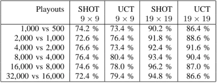
Playouts SHOT UCT SHOT UCT

9 × 9 9 × 9 19 × 19 19 × 19 1,000 vs 500 74.2 % 73.4 % 90.2 % 86.4 % 2,000 vs 1,000 72.6 % 76.4 % 91.8 % 88.6 % 4,000 vs 2,000 76.6 % 73.4 % 92.4 % 91.6 % 8,000 vs 4,000 76.4 % 80.4 % 93.4 % 90.4 % 16,000 vs 8,000 74.6 % 78.0 % 96.2 % 87.0 % 32,000 vs 16,000 72.4 % 79.4 % 94.8 % 86.6 % TABLE 4

Scalability of SHOT versus scalability of UCT for Nogo.

Playouts SHOT SHOT vs UCT SHOT vs UCT

9 × 9 19 × 19

1,000 75.6 % 83.8 % 10,000 75.8 % 90.0 % 100,000 66.8 % 100.0 %

TABLE 5

SHOT versus UCT with same thinking times.

playouts. SHOT uses less memory than UCT since it does not create a node for each playout. Table 3 gives the number of nodes used by SHOT for different number of playouts and different sizes.

Table 4 gives the percentage of wins for SHOT and UCT when they play against themselves with twice the number of playouts. Both SHOT and UCT scale well with more playouts.

Table 5 gives the percentage of wins for SHOT over UCT. The number of playouts of SHOT is fixed and UCT takes at each move the same amount of time as SHOT took at the previous move. We can see that SHOT outperforms UCT at equal time settings.

5

D

In [6] a modification of the UCT algorithm consist-ing of creatconsist-ing a node in memory if it has been sim-ulated at least five times is shown to reduce memory consumption by a factor four while increasing the winning rate to 77 % for Nogo. In comparison, the SHOT algorithm reduces the memory consumption by a factor twenty-five for 9 × 9 Nogo (see table

3) while increasing the winning rate to 66.8 %. For

19 × 19 Nogo, the memory consumption is reduced

by a factor forty while increasing the winning rate to 100.0 %. It is also possible to add slow node

creation to SHOT reducing even more its memory consumption.

We have used a transposition table both in the UCT and in the SHOT algorithms. So both algo-rithms deal in fact with Directed Acyclic Graphs and they both have inconsistent child visit counts.

It is possible that SHOT will work better for games that are Monte Carlo perfect, i.e. increasing numbers of playouts give increasingly accurate re-sults, than for games that are Monte Carlo resistant, i.e. increasing numbers of playouts can actually give worse results. UCT can handle such cases as the tree boundary grows to outweigh the inaccurate playout estimates and revise the estimated value of moves near the root. SHOT eliminates moves from the search so this revision of previous move estimates does not occur, hence it is possible that SHOT will fail to handle games that are Monte Carlo resistant where UCT can.

6

C

In conclusion, SHOT is a viable alternative to UCT. It is parameter free. It scales well since the results are better for 19 × 19 Nogo than for 9 × 9 Nogo and

that increased number of playouts increase the level of play. It uses less memory than standard UCT and beats standard UCT at Nogo for equal time settings. Future works include parallelization on a multi-core machine and on a cluster, applying it to other games and problems and adapting the various im-provements of Monte Carlo Tree Search to SHOT.

A

I thank Abdallah Saffidine who pointed me to the Sequential Halving paper and the anonymous reviewers for helping me improve this paper.

R

[1] Jean-Yves Audibert, S´ebastien Bubeck, and R´emi Munos. Best arm identification in multi-armed bandits. In Adam Tauman Kalai and Mehryar Mohri, editors, COLT, pages 41–53. Omni-press, 2010.

[2] Peter Auer, Nicol`o Cesa-Bianchi, and Paul Fischer. Finite-time analysis of the multiarmed bandit problem. Machine Learning, 47(2-3):235–256, 2002.

[3] Cameron Browne, Edward Powley, Daniel Whitehouse, Simon Lucas, Peter Cowling, Philipp Rohlfshagen, Stephen Tavener, Diego Perez, Spyridon Samothrakis, and Simon Colton. A survey of Monte Carlo tree search methods. Computational Intelligence and AI in Games, IEEE Transactions on, 4(1):1– 43, March 2012.

[4] Tristan Cazenave. Nested monte-carlo search. In Craig Boutilier, editor, IJCAI, pages 456–461, 2009.

[5] Guillaume M. J.-B. Chaslot, Mark H. M. Winands, H. Jaap van den Herik, Jos W. H. M. Uiterwijk, and Bruno Bouzy. Progressive strategies for monte-carlo tree search. New Math-ematics and Natural Computation, 4(3):343–357, 2008. [6] Cheng-Wei Chou, Olivier Teytaud, and Shi-Jim Yen. Revisiting

Monte-Carlo tree search on a normal form game: Nogo. In Applications of Evolutionary Computation, volume 6624 of Lecture Notes in Computer Science, pages 73–82. Springer Berlin Heidelberg, 2011.

[7] R´emi Coulom. Efficient selectivity and backup operators in Monte-Carlo tree search. In Computers and Games, pages 72– 83, 2006.

[8] R´emi Coulom. Computing elo ratings of move patterns in the game of go. ICGA Journal, 30(4):198–208, 2007.

[9] Hilmar Finnsson and Yngvi Bj¨ornsson. Simulation-based ap-proach to general game playing. In AAAI, pages 259–264, 2008. [10] Zohar Karnin, Tomer Koren, and Oren Somekh. Almost optimal exploration in multi-armed bandits. In Proceedings of the 30th International Conference on Machine Learning, pages 1238– 1246, 2013.

[11] Levente Kocsis and Csaba Szepesv´ari. Bandit based Monte-Carlo planning. In 17th European Conference on Machine Learning (ECML’06), volume 4212 of LNCS, pages 282–293. Springer, 2006.

[12] Jean M´ehat and Tristan Cazenave. Combining uct and nested monte carlo search for single-player general game playing. IEEE Trans. Comput. Intellig. and AI in Games, 2(4):271–277, 2010.

[13] Christopher D. Rosin. Nested rollout policy adaptation for monte carlo tree search. In IJCAI, pages 649–654, 2011.