On the use of exact lumpability in partially symmetrical Well-formed Nets
S. Baarir, C. Dutheillet
LIP6, Universit´e Paris 6
8 rue du Capitaine Scott
F-75015 Paris
[email protected]
[email protected]
S. Haddad
LAMSADE, Universit´e Paris 9
Place du Mal De Lattre de Tassigny
F-75016 Paris
[email protected]
J.M. Ili´e
LIP6 & IUT Paris5
143, av. de Versailles
F-75016 Paris
[email protected]
Abstract
Well-formed Nets (WNs) have proved an efficient model for building quotient reachability graphs that can be used either for qualitative or performance analysis. However, local asymmetries often break any possibility of grouping states into classes, thus drastically reducing the interest of the approach. An efficient solution has been proposed for qualitative analysis, which relies on a separate representa-tion of the asymmetries in a so-called control automaton. The quotient graph is then obtained by synchronising the transitions of the WN model with the transitions of the con-trol automaton. In this paper, we improve this approach to quantitative analysis. We show that it can be used to build an aggregated graph that is isomorphic to a Markov chain which verifies exact lumpability. Theoretical consid-erations and practical experiments show that our method outperforms previous approaches.
1
Introduction
Continuous Time Markov Chains (CTMC) are a popu-lar model for evaluating the performance of distributed sys-tems. However, as the complexity of systems increases, the fighting of the so-called combinatorial explosion of the state space becomes more and more critical. A possible approach to tackle this problem is the construction of a lumped CTMC using behavioural symmetries. Such a CTMC offers a com-pact representation of the state space because its nodes are no longer states but classes of states.
Whenever the distributed system is specified by a Well-formed Net (WN) with their restricted syntax (w.r.t. general coloured Petri nets), a symmetry-based quotient structure called Symbolic Reachability Graph (SRG) can be com-puted automatically. On this reduced graph, one solves the reachability problem and more generally the truth of tem-poral logic formulae whenever the atomic propositions of
the formula are symmetrical (e.g. ANDc∈C(p)m(p)(c) =
1). [5] establishes the correctness of this checking in a
gen-eral framework. Moreover, since the SRG verifies strong and exact lumpability criterions, a lumped CTMC is au-tomatically derived from it and any performance result obtained by solving the (usually much larger) complete CTMC, is also computed from the lumped one [4]. The SRG technique works well on highly symmetrical systems. However, in the practice of distributed systems, it is of-ten the case that a system behaves in a symmetric way in most situations, but not all. Any occurrence of asymmetry, even exceptional, reduces drastically the benefices of this approach.
Many approaches were proposed to study such asymmet-rical systems. In [6], the authors propose to adapt the sym-metry rule in accordance with the system specification, to view some groups of almost symmetrical states as symmet-ric. To our knowledge, there is no tool to automate this task thus limiting the practical interest of the approach, more-over no quantitative extension exists.
An other technique named ESRG was proposed in [8], as an extension of the SRG technique. It consists in restraining the symmetries but only on the nodes from which the effects of asymmetric events must be considered. This leads to a reduction in the number of nodes, because one node of the ESRG can represent several classes explicitly represented in the SRG. The ESRG technique is still automatic from the well-formed net specification, and some practical stud-ies show that the constructed CTMC remains compact, in particular whether the refinement operation over an equiv-alence class has no side effect [9]. Nevertheless, the com-putation of the lumped CTMC is not direct [3] : the build-ing of the ESRG is the startbuild-ing point from which a refine-ment process is performed leading to a partial unfolding of nodes up to verify a strong lumpability criteria. Further-more, the exact probabilities of states cannot be expressed since the chosen criteria does not guaranty the equiproba-bility of states lumped under the same node. An additional
extension was proposed in [2] named E2SRG. Although there is no current implementation, the first case studies show than it can be more compact than the ESRG, anyway, it is used to solve reachability problems and the adaptation required to obtain a lumped CTMC is still expected.
In this paper, we propose a new symbolic method for building a lumped CTMC automatically and directly. It is based on a alternative construction, primitively used to check the truth of LTL temporal properties for asymmetric systems [1, 7]. Hence, the system is defined as a synchro-nized product of models: a symmetric system and an event-based automaton to model the symmetric behaviour com-pactly. Symbolic operations are defined in order to split or group symbolic nodes, on-the-fly, during the computa-tion of successors. This allows to adapt, dynamically and locally, the available symmetries for each reachable node. We propose to reuse such an approach for performance pur-poses, moreover an exact lumpability criterion is used to compute the lumped CTMC. Hence, state probabilities can be computed.
The schedule of this paper is the following: section 2 introduces the principles of our method, introducing the no-tion of Partially Symmetrical CTMC; secno-tion 3 is our appli-cation to WNs to obtain an automatic performance analysis tool; section 4 considers a use case extracted from the lit-erature on which we show the benefit of our construction over the RG approach; section 5 contains our conclusions and perspectives.
2
Principles of the Generic Method
2.1
Markov Chains and Lumpability
Lumping of (finite) Markov chains is a useful method for dealing with large chains [10]. The principle is simple: substitute to the Markov chain an “equivalent” one, where each state of the lumped chain is an equivalence class of states of the original one. There are different versions of lumpability related to the fact that the lumpability condition holds for every initial distribution (strong lumpability) or for at least one (weak lumpability).
Definition 1 A CTMC C is defined by a space set S, an in-finitesimal generator Q, and π0, an initial probability distri-bution over S. We note {Xt}t∈IR+ the associated
stochas-tic process. Let C be a CTMC and {Si}i∈I be a partition of the state space. Let Ytbe a random variable defined by
Yt= i ⇔ Xt∈ Si. Then:
• Q is strongly lumpable w.r.t. {Si}i∈I iff ∀π0, {Yt}t∈IR+is a CTMC,
• Q is weakly lumpable w.r.t. {Si}i∈I iff ∃π0 s.t. {Yt}t∈IR+is a CTMC.
Whereas the characterisation of strong lumpability w.r.t. the infinitesimal generator is straightforward, checking for weak lumpability is much harder. Nevertheless, there is a particular case of weak lumpability whose characterisation is easy: the exact lumpability [12].
Proposition 2 Let C be a CTMC and {Si}i∈Ibe a partition of the state space. Then:
• Q is strongly lumpable w.r.t. {Si}i∈I iff ∀i 6= j ∈
I, ∀s, s0∈ S i, P s00∈SjQ(s, s00) = P s00∈SjQ(s0, s00) • Q is exactly lumpable w.r.t. {Si}i∈I iff ∀i 6= j ∈
I, ∀s, s0∈ S i, P s00∈SjQ(s00, s) = P s00∈SjQ(s00, s0). If Q is exactly lumpable w.r.t. {Si}i∈I, then Q is weakly lumpable w.r.t. {Si}i∈I.
Furthermore, exact lumpability fulfills important proper-ties. As for strong lumpability, the infinitesimal generator of the lumped chain is directly computed from the original generator. Starting with a distribution equidistributed on the states of every subset of the partition, the distribution at any time is still equidistributed. Consequently, if the CTMC is ergodic, its steady-state distribution is equidistributed. In other words, with the knowledge of the lumped chain gen-erator, one may compute its steady-state distribution, and deduce (by equidistribution) the steady-state distribution of the original chain. It must be emphasised that this last step is impossible with strong lumpability. The next proposition summarises these results.
Proposition 3 Let C be a CTMC that is exactly lumpable w.r.t. a partition of the state space {Si}i∈I. Let Qlpbe the matrix associated to this lumped CTMC, then:
• ∀i, j ∈ I, ∀s ∈ Sj, Qlp(i, j) = ( P s0∈SiQ(s0, s)) × (|Sj|/|Si|) • If ∀i ∈ I, ∀s, s0 ∈ S i, π0(s) = π0(s0) then ∀t, ∀i ∈ I, ∀s, s0 ∈ S
i, πt(s) = πt(s0), where πtis the proba-bility distribution at time t.
• If Q is ergodic and π is its steady-state distribution
then ∀i ∈ I, ∀s, s0∈ Si, π(s) = π(s0)
2.2
A Model of Partially Symmetrical CTMCs
The model of partially symmetrical systems that we de-velop here is defined as a CTMC obtained by some synchro-nised product between a (symmetrical) CTMC and a control automaton. Let us first formalise this product. Synchronis-ing the behaviour of the two components requires to “label” the CTMC with events.Notation Let C be a CTMC, we associate with each pair of states s 6= s0a label in some alphabet Σ, denoted Λ(s, s0).
a, α a, α a, α a, β a, β a, β a, δ a, δ a, δ b, θ c, θ s0 s1 s2 s3 s6 s 4 s5 l d, θ 0.3 0.3 0.3 0.1 γ = a1 γ = b2
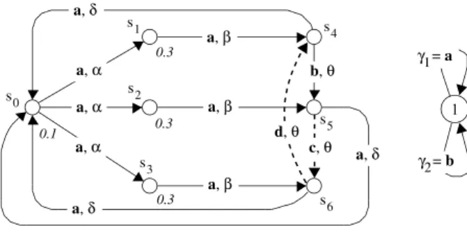
Figure 1. A labeled CTMC and its control au-tomaton
Since the automaton is introduced in order to modify the behaviour of the CTMC, the label of each edge is a predi-cate that selects the events allowed to occur in the current location of the automaton.
Definition 4 Let C be a CTMC, then A = hL, l0, →i a con-trol automaton of C is defined by:
• L, the set of automaton locations, • l0, the initial location,
• →⊆ L × 2Σ× L the transitions of the automaton. A transition (l, γ, l0) will be denoted by l−→ lγ 0.
Fig.1 represents a CTMC and its control automaton. Bold letters are labels, while greek letters represent tran-sition rates. The numbers associated with states are their initial probabilities.
In the synchronised product defined below, the CTMC is the “active” component whereas the automaton inhibits some behaviours of the product. Consequently, the rates (resp. the initial distribution) associated with the product depends only on the rates (resp. the initial distribution) of the CTMC.
Definition 5 Let C be a CTMC and A some control au-tomaton of C. CA = hS × L, π00, Q0i is a CTMC defined by: • ∀s, π0 0(s, l0) = π0(s) ∧ ∀l 6= l0, π00(s, l) = 0 • ∀s 6= s0 ∈ S, ∀l, l0 ∈ L, if l−→ lγ 0∧ Λ(s, s0) ∈ γ then Q0((s, l), (s0, l0)) = Q(s, s0) else Q0((s, l), (s0, l0)) = 0 • ∀s ∈ S, ∀l 6= l0 ∈ L, Q0((s, l), (s, l0)) = 0
In the example of Fig.1, the control automaton actually forbids transitions that are not labelled with a or b. Hence,
CA is obtained from C by removing the dotted arcs.
Formally, the states of CA are pairs (si, l) but as there is only one location in the automaton, we will omit it in the representation of states throughout the example.
From a theoretical point of view, the specification of the system symmetries relies on group theory, applied to the states and the events of the system. The next definition re-calls the appropriate notions.
Definition 6 Let G be a group, with neutral element id and whose internal operation is denoted (•).
• Let E be a set, an operation of G on E is a mapping
from G × E to E s.t. the image of (g, e), denoted by
g.e, fulfills: ∀e ∈ E id.e = e ∀g, g0 ∈ G, (g • g0).e = g.(g0.e)
• The isotropy subgroup of a subset E0 ⊆ E is defined by: GE0 = {g ∈ G | ∀e ∈ E0, g.e ∈ E0}
• Let H be a subgroup of G, the orbit of e by H denoted H.e, is defined by: {g.e | g ∈ H}.
The set of orbits by H defines a partition of E. We simultaneously introduce the notions of symmetrical and partially symmetrical CTMC. Informally, a CTMC is symmetrical w.r.t. some group if the operation of the group on the state space preserves its initial distribution and sto-chastic behaviour. A CTMC is partially symmetrical if it is a synchronised product involving a symmetrical CTMC. Definition 7 A CTMC C is symmetrical w.r.t. G a group operating on S and Σ iff: ∀g ∈ G, ∀s 6= s0 ∈ S, π0(g.s) = π0(s) ∧ Q(g.s, g.s0) = Q(s, s0) and Λ(g.s, g.s0) = g.Λ(s, s0).
Let C be symmetrical w.r.t. G and A be a control au-tomaton of C, then CA is said to be partially symmetrical w.r.t. G.
We associate with each γ occurring in a transition of A a subgroup Hγ ⊆ G defined by: g ∈ Hγ iff ∀a ∈ Σ, a ∈
γ ⇔ g.a ∈ γ.
The size of the subgroup Hγ is an indicator of the sym-metry of the associated edge. When Hγ = G, the edge is “fully” symmetrical whilst when Hγ = {id}, the edge is “fully” asymmetrical.
Back to the example of Fig.1, let G = {id, r, r • r}, where r is defined by :
r.s0= s0 r.s1= s2 r.s2= s3 r.s3= s1 r.s4= s5 r.s5= s6 r.s6= s4
r.a = a r.b = c r.c = d r.d = b
It is easy to verify that G is a group and that the CTMC is symmetrical w.r.t. G. The subgroups associated with the labels of A are Hγ1 = G and Hγ2 = {id}.
2.3
Partially Symmetrical CTMCs and
Lumpa-bility
Given a partially symmetrical CTMC CA, our method builds a smaller (but equivalent) CTMC. However, in order to prove the soundness of this construction, we first intro-duce a CTMC CAG, which is actually bigger than CA.
In CGA, states of CAare replicated in instances, and in-stances are organised in subsets. All the inin-stances that be-long to the same subset must have the same associated lo-cation of the automaton. We will thus consider subsets R of states of the initial CTMC C, and denote (s, l, R) the in-stance of (s, l) s.t. s belongs to R.
Intuitively, given two states (s, l, R) and (s0, l, R) of CG A, any path leading to (s, l, R) may be transformed by the op-eration of some element of G into a path to (s0, l, R).
Definition 8 Let CAbe partially symmetrical w.r.t. G, then the CTMC CAG = hS00, π000, Q00i is inductively defined by:
• The set of states S00is a union of subsets of items de-fined from a set R ⊆ S and a location l by {(s, l, R) |
s ∈ R}, • ∀s ∈ S, ∀l ∈ L, ∀R ⊆ S, if (l = l0∧ R is an orbit by G ∧ s ∈ R) then π00 0(s, l, R) = π00(s, l0) (= π0(s)) else π000(s, l, R) = 0,
• The “initial” subsets of states are {(s, l, R)} s.t. R is
the orbit of s by G ∧ π000(s, l, R) > 0 ,
• If {(s, l, R)} is a subset of states and ∃s∗∈ R, ∃s0∗∈
S, ∃l −→ lγ 0 ∧ Λ(s∗, s0∗) ∈ γ then the subset
{(s0, l0, R0)} with R0= (G
R∩ Hγ).s0∗is another sub-set of states,
• ∀g ∈ GR ∩ Hγ, let s = g.s∗ and s0 = g.s0∗ then
Q00((s, l, R), (s0, l0, R0)) = Q(s, s0) Remarks
1. Let s = g.s∗ and s0 = g.s0∗, since Q(s, s0) =
Q(g.s∗, g.s0∗) = Q(s∗, s0∗), the transition rate does not depend on the chosen pair.
2. Furthermore the above subset construction does not depend on the choice of s∗ and s0∗ in the following sense. Let us pick some s0 ∈ (GR ∩ Hγ).s0∗, thus
s0 = g.s0∗with g ∈ G
R∩ Hγ. Define s = g.s∗, then
s ∈ R(⊇ GR.s∗) and Λ(s, s0) ∈ γ. Now it is routine to show that (GR∩ Hγ).s0 = (GR∩ Hγ).s0∗. Fig.2 describes CTMC CAGfor our example. Dotted rec-tangles represent the subsets of states. The initial subsets are those with associated orbits S0 = {s0} and S123 =
s 0, S0 s 1, S123 s 2, S123 s 3, S123 s 4, S456 s 5, S456 s 6, S456 s 5, S5 α α α β β β θ δ δ δ δ G G G { id } Figure 2. CTMCCG A S 123 S456 S 0 3.α β θ/3 S5 δ δ 0.1 0.9 Figure 3. CTMC(CG A)lp
{s1, s2, s3}. A group is associated with each subset: the group is G for the initial subsets and remains G for the con-structed subsets until there is a synchronisation with γ2. At that moment, the group is reduced to identity by intersec-tion with Hγ2 and the constructed subset contains a single state. As a consequence, there are two instances of s5in the resulting CTMC, each with a different associated orbit.
In fact, the stochastic process we want to build is ob-tained by forgetting the instances and only memorising the subsets.
Definition 9 Let CAbe partially symmetrical w.r.t. G, then the stochastic process (CAG)lpis defined by: Xlp
t = (R, l) iff Xt00∈ {(s, l, R)}.
The resulting process for the example is given in Fig.3. The initial distribution and the transition rates are computed according to Prop.3.
The next proposition is the theoretical core of our method. It states that (CAG)lp is obtained from C
A by the inverse of a (strong) lumping followed by an exact lump-ing.
Proposition 10 Let CA be partially symmetrical w.r.t. G, then:
• Denoting (s0, l0) . . . , (sn, ln) the state space of CA,
CA is a strong lumping of CAG w.r.t. the partition
• Denoting {(R0, l0), . . . , (Rk, lk)} the state space of
(CG
A)lp, (CAG)lp is an exact lumping of CAG w.r.t. the partition {(s, l0, R0)}s∈R0, . . . , {(s, lk, Rk)}s∈Rk
Proof
Let (s, l) be a state of CAand let (s, l, R) be a state of CAG, we show that there is a bijective mapping from the transi-tions out of (s, l) onto the transitransi-tions out of (s, l, R). Due to the above remark we suppose that (s, l, R) is examined when looking for successors of {(s0, l, R) | s0 ∈ R} in Def. 8. Then ∃s0, ∃l −→ lγ 0s.t. Λ(s, s0) ∈ γ ⇔ ∃R0, ∃s0 ∈
R0, ∃l −→ lγ 0 s.t. Λ(s, s0) ∈ γ with R0 = (G
R∩ Hγ).s0. Since this mapping preserves the rate of the transitions the condition of Prop. 2 for strong lumpability is fulfilled.
Let (s1, l, R) and (s2, l, R) be two states of CAG, we show that there is a bijective mapping from the input transitions of (s1, l, R) onto the input transitions of (s2, l, R). Let
(v1, l0, R0) be such that ∃l0 γ−→ l and Λ(v1, s1) ∈ γ. Due to the same remark, ∃g ∈ GR0 ∩ Hγ s.t. s2 = g.s1. Now
define v2 = g.v1, then v2 ∈ R0 and Λ(v2, s2) ∈ γ. This implies the existence of the required mapping. Since this mapping preserves the rates of transitions, the condition of Prop. 2 for exact lumpability is fulfilled. ♦
Our generic method can now be described. Assume first that the CTMC CAassociated with the high-level model M we want to analyse is partially symmetrical. Assume also that we are able to compute directly (CAG)lpfrom M. Note
πtthe unknown distribution of CAat time t and π(lp)t the (computed) distribution of (CAG)lpat time t. Then π
t(s, l) =
P
s∈R(1/|R|) × π (lp)
t (R, l). The equality also holds for the steady-state distributions. The next section will show that the assumptions above are satisfied in the framework of SWNs. In fact, we believe that our method is applicable to any model where symmetry is automatically handled.
Although theoretically difficult, we can give some hints of how the space complexity decreases using our approach. In the lumped CTMC, the original states have been sub-stituted by subsets. Note that these subsets may intersect. However these subsets are always the orbit of a state by a subgroup of G. Thus, the larger these subgroups, the bet-ter the method. Note that each time a new subset is built, the group is reduced (by intersection with Hγ) and then is enlarged by implicitly substituting to G ∩ Hγ the isotropy subgroup of the subset. Interpreting this phenomenon at the model level, we deduce that the complexity reduction fac-tor is high whenever the effect of an asymmetrical event is forgotten in a close future. Experimentations will illustrate this interpretation.
3
Application to Stochastic Well-formed Nets
3.1
Presentation of the model and the symbolic
reachability graph
WNs are a model of high-level Petri nets whose syntax has been the starting point of numerous efficient analysis methods. Below, we describe the main features of WNs. The reader can refer to [4] for a formal definition:
• In a WN (and more generally in high-level nets) a
colour domain is associated with places and transi-tions. The colours of a place label the tokens contained in this place, whereas the colours of a transition define different ways of firing it. In order to specify these fir-ings, a colour function is attached to every arc which, given a colour of the transition connected to the arc, determines the number of coloured tokens that will be added to or removed from the corresponding place. Fi-nally the initial marking is defined by a multi-set of coloured tokens in each place.
• A colour domain is a cartesian product of colour
classes which may be viewed as primitive domains. This product is possibly empty (e.g., a place which contains neutral tokens) and may include repetitions (e.g., a transition which synchronises two colours in-side a class). A class can be divided into static sub-classes. The colours of a class have the same nature (processes, resources, etc.), whereas the colours in-side a static subclass have the same potential behaviour (batch processes, interactive processes, etc.).
• A colour function is built by standard operations
(lin-ear combination, composition, etc.) on basic functions. There are three basic functions: a projection which se-lects an item of a tuple and is denoted by a typed vari-able (e.g., p, q); a diffusion, a constant function which returns the bag composed by all the colours of a class or a subclass and is denoted SC where C is the cor-responding (sub)class; and a successor function which applies on an ordered class and returns the colour fol-lowing a given colour.
• Transitions and colour functions can be guarded by
ex-pressions. An expression is a boolean combination of atomic predicates. An atomic predicate either identi-fies two variables [p = q] or restricts the domain of a variable to a static subclass.
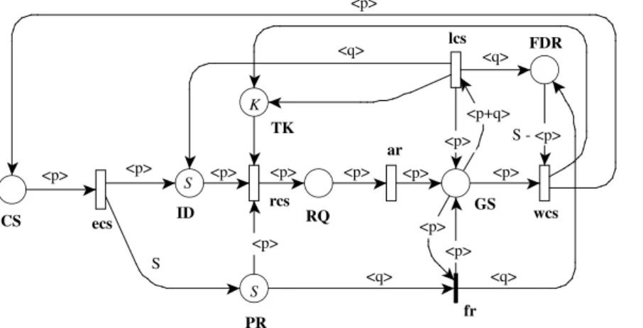
We illustrate these features on the WN model in Fig. 4. It represents a distributed critical section algorithm. There is a single class C: the set of processes that interact in the system. The colour domain of all the places of the net is
CS ID RQ GS PR FDR TK ecs rcs lcs ar fr wcs <p> S S K <p> <p> <p> <p> <p> <q> <q> <p> <q> <q> S - <p> S <p> lcs [p > q] q ¬ lcs <p> <p> <p+q> <p> <p>
Figure 4. A WN model of a distributed critical section with its control automaton
there is a single class, the constant function representing the set of all processes will be simply denoted S.
Initially, all processes are idle (place ID), meaning that they do not request the critical section. The firing of transi-tion rcs represents a process requesting the critical sectransi-tion. Only up to K processes can apply simultaneously and ad-ditional candidacies are rejected, which is represented by K tokens in place TK. This constant K depends on the para-meters of the physical access to the system (e.g., network topology).
As soon as a process reaches the state where others are aware of its request (place GS), no process can become can-didate any longer : permissions for applying are removed from place PR by the firing of fr (with priority over other transitions). If there are several candidates, i.e., the num-ber of tokens in places RQ and GS is greater than one, all but one will be discarded through the successive firings of lcs. When there is more than one token in GS, the firing of lcs non deterministically chooses two of them and discards one. When there is only one left (which is guaranteed by the number of tokens in FDR), it can enter the critical section (place CS) by firing wcs. When the process releases the crit-ical section (firing of transition ecs), all processes become idle again and a new round can start.
The implicit symmetry of a WN is associated with a group Gsrg operating on colour classes (and by extension on markings and firing instances). Gsrg is the intersec-tion of the isotropy subgroups of static subclasses. In other words, any permutation in Gsrg maps any static subclass onto itself. Given a marking m and a permutation g of Gsrg, the behaviour of the net from the marking g.m is the same as the behaviour from m up to permutation g. We say that this two markings are equivalent and we use ˆm as a sym-bolic representation for the orbit Gsrg.m.
The symbolic reachability graph (SRG) construction lies on symbolic markings, namely a compact representation for
a set of equivalent ordinary markings. A symbolic marking is a generic representation, where the actual identity of to-kens is forgotten and only their distributions among places are stored. Tokens with the same distribution and belong-ing to the same static subclass are grouped into a so-called dynamical subclass.
In the rest of the paper, we will use a notation where only the cardinality of dynamical subclasses is represented. For instance, in the case where C = {c1, c2}, the symbolic marking ˆm = ID(1) + RQ(1) will represent the two ordi-nary markings ID(c1) + RQ(c2) and ID(c2) + RQ(c1).
Then, the SRG can be constructed automatically using a symbolic firing rule that directly applies on symbolic mark-ings [4].
Various behaviourial properties may be directly checked on the SRG. Furthermore, this construction leads to an ef-ficient performance evaluation of Stochastic WNs (SWNs). A SWN is obtained from a WN by associating an expo-nentially distributed delay with every transition. The rate of this transition may depend on the static subclasses to which the firing colours belong. The key result is that the related CTMC may be (strongly and exactly) lumped and that the lumped CTMC is isomorphic to the SRG. As for stochastic Petri nets, the definition can be extended with im-mediate transitions and a similar result holds for the semi-Markovian process.
However, the SRG approach is not adapted when deal-ing with asymmetrical systems: in our example, let us now decide that when several processes request the critical sec-tion, the selected process is the candidate with the highest identity. Hence, the set of bindings of transition lcs must be restricted to pairs (p, q) s.t. p > q. In SWNs, this could be done by adding a guard to transition lcs. Yet, the only way to express this guard is to partition colour class C into static subclasses reduced to singletons {ci}. Then, the guard is
W
isomor-phic to the ordinary reachability graph (RG) and there is no more gain in complexity.
3.2
The Dynamic Symbolic Reachability Graph
(DSRG) construction
The drawback of the SRG approach is that asymmetries are defined statically and taken into account throughout the construction of the graph. Yet, very often, they have only local effects. Back to our example, except when a process is involved in a selection, there is no need to know its ac-tual identity. Thus, the asymmetry is local to the selection process.
Hence, the challenge is to adapt the method of Section 2, where asymmetrical behaviours are treated as locally as possible, to the SWN model.
The approach we develop here reuses and extends the SWN symbolic framework to automatise the construction of the lumped CTMC (CAG)lp. We call DSRG the symbolic structure that represents this CTMC. It is based on a sym-bolic representation for {(s, l, R) | s ∈ R} and a firing rule that directly applies on it.
The symmetrical features of the system are captured by the SWN and the asymmetries are represented by a control automaton. The definition of the latter requires only that we precise alphabet Σ. Since the CTMC is isomorphic to the RG, the labels associated with it are the firing instances of the transitions. Formally, Σ = {(t, c) | t ∈ T ∧ c ∈ C(t)} where T is the set of transitions of the SWN and C(t) is the colour domain of t. Labels of the automaton are subsets of
Σ. In our example, there are two labels: ¬lcs = {(t, c) |
t 6= lcs ∧ c ∈ C(t)} and lcs[p > q] = {(lcs, (p, q)) |
(p, q) ∈ C2∧ p > q}.
Symbolic representation of states in DSRG
In SWNs, a state s is a marking m, and we want a sym-bolic representation for the set {(m, l, R) | m ∈ R}, s.t.
R = G0.m∗, G0 a subgroup of G and m∗any marking of
R. We choose a notation similar to that of the SRG, namely hD, ˆm, li, where D is the set of orbits by G0 of the colour classes and ˆm is the symbolic representation of G0.m. We call this representation symbolic state.
The symbolic state defined by D = {{c1, c2}, {c3}},
ˆ
m = ID({c1, c2}0) + RQ({c1, c2}1 + {c3}) and an associated location l represents the set
{(m1, l, S12), (m2, l, S12)} s.t. m1= ID(c1) + RQ(c2+ c3) and m2= ID(c2) + RQ(c1+ c3).
Symbolic firing rule in DSRG
Let l −→ lγ 0be a transition of the control automaton and
Hγ be the subgroup of permutations associated to γ. We want to compute the successors of node hD, ˆm, li w.r.t. γ, by use of the symbolic firing rule of SWNs.
The key observation is that the restriction imposed by
γ can be expressed by a SWN guard that is injected
dy-namically to the treated net. Thus, Hγ must be represented as a colour class partition in static subclasses, namely Dγ. These static subclasses are used to express the above guard. In our example, the label lcs[p > q] splits C in singletons in order to express p > q as a SWN guard attached to lcs.
To be able to perform a classical symbolic firing, we have to compute a new partition D0 = D ∩ Dγ and refine
hD, ˆm, li in a family F = {hD0, cm
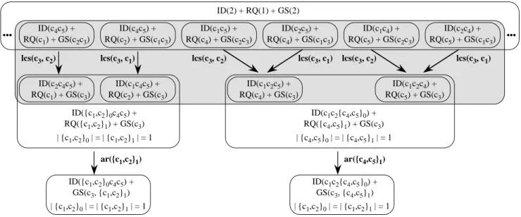
1, li, hD0, cm2, li, . . .}. In the second line of Fig. 5, six among the thirty symbolic markings of the partition are shown. In this case, due to the partition in singletons, each symbolic representation in-cludes only one ordinary state.
Now, the classical SRG symbolic firing rule can be ap-plied on each element of F with the additional control in-duced by the label. This control is performed at the sym-bolic level due to the previous splitting.
Back to the generic method, we have built the subset
{(s, l0, R0)} with R0 = (G
R∩ Hγ).s0∗. The substitution of GR∩ Hγ by the isotropy subgroup GR0 is explicitly
per-formed in SWNs as follows. Two static subclasses reduced to a single dynamic subclass and with the same distribution in places are merged. Observe that the subset of states is unchanged whereas the static partition is rougher. For in-stance in any marking of the third line of Fig. 5, the three static subclasses (here reduced to a colour) in place ID, can be merged in a single one.
Computation of the transition rates of the lumped CTMC
Using the method described in section 2, the graph we obtain is isomorphic to a lumped Markov chain, whose rates can be computed directly from information obtained during the construction of the DSRG. From the first equation of proposition 3, we know that the transition rate between two classes depends on the cardinalities of the source and desti-nation classes, namely Siand Sj, and the input rate of any state s of the destination class, i.e.,Ps0∈SiQ(s0, s). Let us
consider the contribution toPs0∈SiQ(s0, s) of an arc
rep-resenting the firing of a transition t. After the splitting step, a symbolic instantiation of t is possible for all or none of the markings that still belong to the same symbolic repre-sentation. Assume that such a firing of t is possible in a split representation and let us denote Si0the ordinary states contained in this representation and |Si0| the number of such
states. The global rate out of Si caused by the firing we consider is |Si0|.e.µ(t), where e is the number of ordinary firings represented by the symbolic firing of t and µ(t) is the rate of transition t. Note that if different bindings of t have different rates, this can be taken into account in the con-trol automaton, thus we consider here only the case where equivalent bindings have equivalent rates.
ID(2) + RQ(1) + GS(2) ID(c4c5) + RQ(c1) + GS(c2c3) ID(c4c5) + RQ(c2) + GS(c1c3) ID(c2c5) + RQ(c4) + GS(c1c3) ID(c2c4) + RQ(c5) + GS(c1c3) ID(c1c5) + RQ(c4) + GS(c2c3) ID(c1c4) + RQ(c5) + GS(c2c3) ID(c1c4c5) + RQ(c2) + GS(c3) ID(c2c4c5) + RQ(c1) + GS(c3) ID(c1c2c4) + RQ(c5) + GS(c3) ID({c1,c2}0c4c5) + RQ({c1,c2}1) + GS(c3) ID(c1c2{c4,c5}0) + RQ({c4,c5}1) + GS(c3) | {c1,c2}0 | = | {c1,c2}1 | = 1 | {c4,c5}0 | = | {c4,c5}1 | = 1 ar({c1,c2}1) ar({c4,c5}1) ID({c1,c2}0c4c5) + GS(c3, {c1,c2}1) | {c1,c2}0 | = | {c1,c2}1 | = 1 ID(c1c2{c4,c5}0) + GS(c3, {c4,c5}1) | {c1,c2}0 | = | {c1,c2}1 | = 1 lcs(c3, c2) lcs(c3, c1) lcs(c3, c2) lcs(c3, c1) lcs(c3, c2) lcs(c3, c1) ID(c1c2c5) + RQ(c4) + GS(c3) ••• •••
Figure 5. Firing and grouping
As all the states in Sjhave the same input rate, this rate is given by |S0i|.e.µ(t)/|Sj|. Hence Qlp(i, j) = |S
0 i|.e.µ(t)
|Si| . The computations of the number of ordinary markings con-tained in a symbolic marking and the number of ordinary firings represented by a symbolic firing for the SRG are de-tailed in [4].
3.3
Optimisations for WNs
In this paragraph, we show that the SWN formalism leads to further optimisations of the generic method. The first one consists in grouping the symbolic representations obtained after a symbolic firing provided that the condition for exact lumpability still holds. This optimisation is feasi-ble since the transition rates of the lumped CTMC can be computed on-the-fly. It appears that after this optimisation, the overall strategy for choosing the next symbolic firing af-fects the size of the lumped CTMC (which was not the case previously). Hence our second optimisation heuristically tries to minimize this size.
Grouping of symbolic markings
In fact, this optimisation was already proposed in [1]. However, the conditions of this merging were weaker as they require to preserve the existence of particular paths in the graph. When dealing with performance evaluation, states can no longer be grouped on qualitative criteria only. Input rates must be taken into account, which often restricts the possibilities of grouping. For the sake of simplicity, we will consider here a uniform rate of 1.0 for any binding of transition lcs and use this example to illustrate the problems that may arise. Let P = 5 be the number of processes and
ID(2) + GS(3) ID(3) + GS(2) ID(3) + GS(1) + RQ(1) ID(2) + GS(2) + RQ(1) lcs ar lcs
Figure 6. Firings to be considered
K = 3 the maximum number of simultaneous candidacies.
Fig. 6 represents the distributions of tokens in significant places and the firings of transitions we are going to detail throughout this section.
We consider the firing sequence starting from the sym-metrical representation where two processes are idle, one has sent a request and two are ready to perform a selection. The synchronisation of the SWN and the control automaton for the firing of transition lcs ends up in a complete refine-ment of the source marking, as the only symmetry that is compatible with the label lcs[p > q] is the identity. For each of these refined markings, there is exactly one pos-sible binding of transition lcs, because lcs[p > q] fixes the order between p and q. A significant subset of the re-fined markings and the corresponding firings is represented in the shaded part of Fig. 5. At this point, we try to group the markings that are obtained from the firing. Obviously, whichever pair we consider, there exists a permutation tween the markings. But even if all the source markings be-long to the same class, not any pair satisfies the exact lumpa-bility condition. Looking only at the represented markings, as we have considered a uniform rate of 1.0 for transition
lcs, the only possibility we have is to group the two right markings, and also the two left ones. The shaded part is then removed, and only the white portion is actually stored in the graph. The notation {ci, cj}k defines a partition of the set {ci, cj}: in the left class for instance, RQ({c1, c2}1) with |{c1, c2}1| = 1 means that either c1or c2is in RQ, the other one belongs to {c1, c2}0, hence it is in place ID. We have already detailed how transition rates associated with arcs are computed. Once this is done, we can compute the transition rates between classes using the formula in Section 2.
From the classes we have built, we can fire transition ar. There is no restriction associated with this transition in the control automaton, hence we use the classical firing rule of SWNs from which we can directly build the class of reached markings : whatever the identity of the token in RQ, it is moved to place GS.
Overall strategies for construction
We show now that the previous optimisation requires an efficient strategy for choosing the next transition to fire, in order to minimize the size of the lumped CTMC. For in-stance, what may happen is that a set of markings that is represented by a single class is reached through another fir-ing that prevents them from stayfir-ing in the same group. We show an example in Fig. 7: the class with two processes in place ID and three in place GS enables transition lcs. Its different bindings will lead to any combination of two processes in place GS, except (c1c2), and the three other processes in place ID. We already encountered such a con-figuration in the previous firing sequence. However, we did not have to separate the markings where GS contained (c3c4) or (c3c5) because they were obtained from a sym-metrical firing, which guaranteed that they had the same in-put rate. We can see that this is no longer true when we take this firing into account. If we have not built any firing from the subclass representing the two markings yet, we re-move the subclass and dispatch its input rate on the individ-ual markings. If we have already built the firings, we keep both representations because removing the subclass could have a domino effect on the downward part of the graph. To avoid as much as possible the construction of redundant subclasses, we try to favour the construction of individual markings first by firing asymmetrical prior to symmetrical transitions.
As the construction of subclasses and individual mark-ings may happen anyway, the same state can be represented several times in the graph. In this case, for any class it ap-pears in, we compute the probability of a state of the class, which is obtained by dividing the probability of the class by its cardinality. The actual probability of the state will then be computed by summing the values obtained for any class it appears in. ID(2) + GS(3) lcs ID(c1c2c4) + GS(c3c5) ••• ID(c ••• 1c2c5) + GS(c3c4) lcs
Figure 7. Construction of included markings
3.4
Extension to immediate transitions
When the model includes immediate transitions, the un-derlying stochastic process becomes semi-Markovian.We use the embedded Markov Chain approach to compute steady-state probabilities. We thus handle a discrete-time process, but the exact lumpability criterion still holds on this process and the steady-state probabilities can be computed in the same way as in the continuous-time case.
Special care must be taken however if some class enables both timed and immediate transitions. This happens for in-stance if all the colours in a class have had a symmetrical behaviour so far, and an asymmetrical immediate transition is enabled for some of them in the current class of mark-ings, while a timed transition is enabled for others. In this case, the class must be split into a vanishing subclass and a tangible one. But as we consider only input rates for test-ing the lumptest-ing condition, this splitttest-ing has no effect on the upward part of the graph.
4
Numerical Results
To test the efficiency of our method, we have imple-mented the DSRG on the same kernel as the standard (S)RG. For that, we have modified the GreatSPN package (www.di.unito.it/∼greatspn) on which the (S)RG is imple-mented. Hence, one can specify a SWN to obtain the results of both constructions. The machine used for our tests is a PC/Linux of 3.2 GHz and 3 Gb of RAM.
In this section, we will consider the net of Fig. 4 once again. An examination of its structure would show that the complexity of the model is strongly related to the settings of parameters P and K, respectively the number of processes in the system and the number of processes that are able to concurrently apply for the critical section (K ≤ P ). For instance, by focusing on the two places RQ and GS, one notes that increasing K acts on the number of tokens in these two places, while increasing P widens the possibilities of choosing the identities of the tokens that they contain.
Let us now compare the effects of increasing the values of P and K on the (S)RG and DSRG methods.
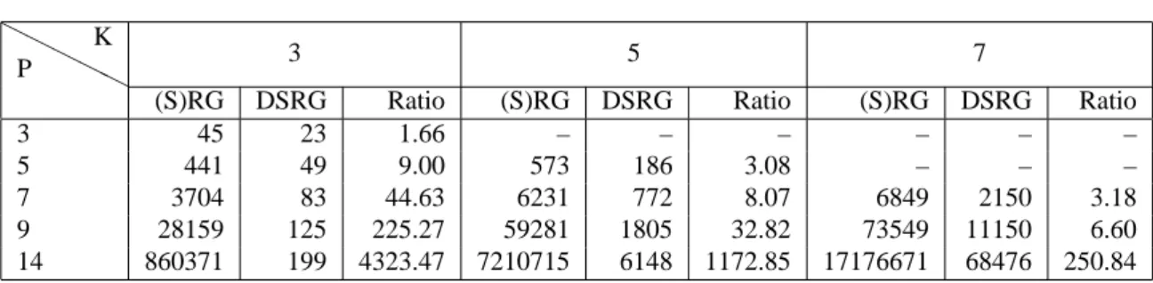
Table 1 summarizes our experiments. The columns noted (S)RG (respectively DSRG), shows the number of constructed nodes in the (S)RG (respectively DSRG) struc-ture for a given K and P .
Table 1. Size of the (S)RG and DSRG w.r.t. PandK HH HHH P K 3 5 7
(S)RG DSRG Ratio (S)RG DSRG Ratio (S)RG DSRG Ratio
3 45 23 1.66 – – – – – –
5 441 49 9.00 573 186 3.08 – – –
7 3704 83 44.63 6231 772 8.07 6849 2150 3.18
9 28159 125 225.27 59281 1805 32.82 73549 11150 6.60
14 860371 199 4323.47 7210715 6148 1172.85 17176671 68476 250.84
For a fixed value of K and w.r.t. the increasing of P, we observe empirically that the RG grows exponentially whereas the DSRG progresses almost linearly. This is eas-ily explained by the fact that the complexity induced by the different possibilities to select K concurrent processes are explicitly represented in the (S)RG, whereas they are sym-bolically represented in the DSRG. More precisely, in the DSRG, no asymmetry among processes is taken into ac-count until asymmetrical transition lcs is enabled. More-over, the symbolic grouping optimisations make it possible to regain part of the symmetries that are lost due an asym-metrical firing.
For a fixed value of P, one should observe that the sizes of both structures increase exponentially. However, there is a limitation as the number K is closed to its maximum, P . Such a limitation is clearly seen for the (S)RG, where the rate of augmentation of the size decreases for any given P . Unfortunately, we cannot compare the DSRG to the (S)RG since the effect of our symbolic grouping operations is con-textual (thus not controllable).
Nevertheless, we are able to compare the relative gain of our method (see columns noted Ratio of Table 1). Thus, the ratio between the two structures progresses exponen-tially w.r.t. P and this proves the efficiency of our approach. W.r.t. K, a regression can be noted, it is caused by the ex-ponential observed above.
Last, we notice that the DSRG construction time is relatively high. As an example for values P = 9 and
K = 5, the building requires 275 seconds, while it
requires 126 seconds for the RG. In fact, 47% of the total construction time is spent in comparisons of sets of colours and this percentage remains constant for all constructions. Therefore, we are working to integrate cache techniques in our software to solve this problem.
5
Conclusion and perspectives
We have proposed a new automatised and symbolic method to build a lumped CTMC which verifies exact lumpability. Our method is generic and should be
applica-ble to a large category of performance models. Moreover, in practical cases, the additional specification of the control automaton remains straightforward. Applied to a (common) use case, the DSRG construction appears to be very rele-vant in terms of used memory. We need now to improve our tool in order to gain efficiency in time. Our next research perspective will be to extend the proposed method to prob-abilistic model checking.
References
[1] S. Baarir, S. Haddad, and J.-M. Ili´e. Exploiting Partial Symmetries in Well-formed nets for the Reachability and the Linear Time Model Checking Problems. In Proc. of WODES’04 - IFAC Workshop on Discrete Event Systems, part of 7th CAAP, Reims - France, 2004. Springer Verlag. [2] C. Bellettini and L. Capra. A quotient graph for
asymmet-ric distributed systems. 12th IEEE Int. Symp. on Modeling, Analysis, and Simulation of Computer and Telecommunica-tion Systems (MASCOTS), pages 560–568, october 2004. [3] L. Capra, C. Dutheillet, G. Franceschinis, and J.-M. Ili´e.
Ex-ploiting partial symmetries for Markov chain aggregation. E. Notes in Theoretical Computer Science, 39(3), 2000. [4] G. Chiola, C. Dutheillet, G. Franceschinis, and S.
Had-dad. Stochastic well-formed coloured nets for symmetric modelling applications. IEEE Transactions on Computers, 42(11):1343–1360, nov 1993.
[5] E. Clarke, R. Enders, T. Filkorn, and S. Jha. Exploiting Sym-metry in Temporal Logic Model Chacking. Formal Methods and System Design, 9:77–104, 1996.
[6] E. A. Emerson and R. J. Trefler. From Asymmetry to Full Symmetry: New Techniques For Symmetry Reduction in Model Checking. In Proc of CHARME99, Lecture Notes in Computer Science, pages 142–156, Bad Herrenalb - Ger-many, Sept. 1999. Springer Verlag.
[7] S. Haddad, J. Ili´e, and K. Ajami. A model checking method for partially symmetric systems. In Proceedings of FORTE/PSTV’00, pages 121–136, Pisa, Italy, Oct. 2000. Kluwer Academic Publishers.
[8] S. Haddad, J. Ili´e, M. Taghelit, and B. Zouari. Symbolic Reachability Graph and Partial Symmetries. In Proc. of the 16th
Intern. Conference on Application and Theory of Petri Nets, volume 935 of LNCS, pages 238–257, Turin, Italy, June 1995. Springer Verlag.
[9] J. Ili´e, S. Baarir, M. Beccuti, S. Donatelli, C. Dutheillet, G. Franceschinis, R. Gaeta, and P. Moreaux. Extended SWN Solvers in GreatSPN. In Tool paper for the 1st Int. Conf. on Quantitative Evaluation of Systems (QEST’04), LNCS, Twente, Netherland, 2004. Springer Verlag.
[10] J. Kemeny and J. Snell. Finite Markov chains. New York, NY, 1960. D. Van Nostrand-Reinhold.
[11] G. Rubino and B. Sericola. On weak lumpability in Markov chains. Journal of Appl. Prob., 26:446–457, 1989.
[12] P. J. Schweitzer. Aggregation methods for large Markov chains. In Proceedings of the International Workshop on Computer Performance and Reliability, pages 275–286. North-Holland, 1984.