A new bound for solving the recourse problem
of the 2-stage robust location transportation
problem
V. Gabrel, C. Murat, N. Remli, M. Lacroix
1 LamsadeUniversit´e Paris-Dauphine
Place du Mar´echal De Lattre de Tassigny, 75775 Paris Cedex 16, France
Abstract
In this paper, we are interested in the recourse problem of the 2-stage robust loca-tion transportaloca-tion problem. We propose a soluloca-tion process using a mixed-integer formulation with an appropriate tight bound.
Keywords: Location transportation problem, robust optimization, mixed-integer linear programming.
1
Introduction
Robust optimization is a recent methodology for handling problems affected by uncertain data, and where no probability distribution is available. In robust optimization two decisional contexts are considered for taking decision under uncertainty. The first one is the single-stage context where the decision-maker has to select a solution before knowing the realization (values) of the uncertain parameters. Generally, the single-stage approaches provide the worst case
1
solutions (Soyster [18]) that are very conservative and far from optimality in real-world applications. The maximum regret criterion can also be applied
as a single-stage approach to problems affected by uncertain costs (see [10],
[13], [14], [15] to name a few). The second approach concerns the multi-stage
context (or dynamic decision-making) where the information is revealed in stages, and some recourse decision can be made. The multi-stage approach
was firstly introduced by Ben-Tal et. al. [2], and initial focus was on two-stage
decision making on linear programs with uncertain feasible set. Note that the formulations obtained following this approach are generally untractable.
In this paper, we are interested in a robust version of the location trans-portation problem with an uncertain demand using a 2-stage formulation.
Recently, Atamturk and Zhang [1] used a two-stage robust optimization in
network flow and design problem to obtain a good approximation of the
ro-bust solutions. Furthermore, Thiele et. al. [19] describe a two-stage robust
approach to address general linear programs affected by uncertain right hand side. The robust formulation they obtained is a convex (not linear) program, and they propose a cutting plane algorithm to exactly solve the problem. In-deed, at each iteration, they have to solve an NP-hard recourse problem on an exact way, which is time-expensive. Here, we go further in the analysis of the recourse problem of the location transportation problem, in particular we define a tight bound for the mixed-integer reformulation.
The paper is organized as follows: in Section2, the nominal location
trans-portation problem is introduced and its corresponding 2-stage robust
formu-lation. A mixed integer program is then proposed in Section 3 to solve the
quadratic recourse problem with a tight bound. Finally, in Section 4, the
results of numerical experiments are discussed.
2
Robust location transportation problem
We consider the following location transportation problem: a commodity is to be transported from each of m potential sources, to each of n destinations. The
sources capacities are Ci, i = 1, . . . , m and the demands at the destinations are
βj, j = 1, . . . , n. To guarantee feasibility, we assume that the total sum of the
capacities at the sources is greater than or equal to the sum of the demands at the destinations. The fixed and variable costs of supplying from source
i = 1, . . . , m are fiand di, respectively. The cost of transporting one unit of the
commodity from source i to destination j is µij. The goal is to determine which
sources to open (ri), the supply level yi and the amounts tij to be transported
location transportation problem is the following linear program, (T ): (T ) min m P i=1 diyi+ m P i=1 firi+ m P i=1 n P j=1 µijtij s.t. n P j=1 tij ≤ yi i = 1 . . . m m P i=1 tij ≥ βj j = 1 . . . n yi ≤ Ciri i = 1 . . . m ri ∈ {0, 1}, yi, tij ≥ 0 i = 1 . . . m, j = 1 . . . n
In case of uncertainty on the demands, we model each demand by intervals,
such that every βj varies in [βj− ˆβj, βj+ ˆβj] where βj represents the nominal
value of βj and ˆβj ≥ 0 its maximum deviation. Clearly, each demand βi can
take on any value from the corresponding interval regardless of the values taken
by other coefficients. We denote (Tβ) the location transportation problem for
a given β ∈ [β − ˆβ, β + ˆβ], with a nonempty feasible set. Finally, we denote
Z(Tβ) the optimal value (bounded value) of (Tβ) for a given β.
Following the approach suggested by [1], [8] and [19], which is a natural
adaptation of the original Bertsimas and Sim approach (see [4],[3]), we define
a parameter Γ, called the budget of uncertainty representing the maximum range of uncertain demands that can deviate from their nominal values. We have Γ ∈ [0, n]. For Γ = 0, every right hand side is equal to its nominal value, while Γ = n leads to consider the problem with the worst demands.
We are interested in solving a robust version of the problem (Tβ) with a
2-stage formulation. Indeed, the problem is to determine the minimum cost of
choosing the facility i, i = 1, . . . , m to be opened (with the ri variables), and
the supply level yi, such that the worst demand is satisfied with a minimum
cost. In this case, ri and yi variables are decided before the realization of the
uncertainty (first stage decisions), while the tij variables represent the recourse
variables to decide after the demands are revealed (second stage decisions). The robust problem is the following:
TRob(Γ) min yi≤Ciri, i=1...m yi≥0, ri∈{0,1} { m P i=1 diyi+ m P i=1 firi+ max β∈U n min P j=1 tij≤yi, i=1...m m P i=1 tij≥βj, j=1...n tij≥0, i=1...m, j=1...n m P i=1 n P j=1 µijtij} where U = {β ∈ Rn: βj = βj+ zjβˆj, j = 1, . . . , n, z ∈ Z} (1) and Z = {z ∈ Rn : n X j=1 |zj| ≤ Γ, − 1 ≤ zj ≤ 1, j = 1 . . . n}. (2)
The problem TRob(Γ) is a convex optimization problem that can be solved
using Kelley’s algorithm (see [11], [19]) that optimizes iteratively the master
problem and the recourse problem by generating cuts. In this work, we focus on the recourse problem, namely
P (y, Γ) max n P j=1 |zj|≤Γ −1≤zj≤1, j=1,...,n min n P j=1 tij≤yi, i=1...m m P i=1 tij≥βj+ ˆβjzj, j=1...n tij≥0, i=1...m, j=1...n m P i=1 n P j=1 µijtij
At optimality Z(P (y, Γ)) represents the transportation cost value for a fixed capacity level y, and Γ worst deviations. Furthermore, we assume that P (y, Γ) has a nonempty feasible set.
Because of the sense of the constraints of P (y, Γ), the optimal values of the
zj variables will never be negative, and necessarily belong to [0, 1]. Moreover,
dual (since the problem is always feasible): Q(y, Γ) max − m P i=1 yiui+ n P j=1 βjvj + n P j=1 ˆ βjvjzj s.t. vj− ui ≤ µij i = 1 . . . m, j = 1 . . . n n P j=1 zj ≤ Γ 0 ≤ zj ≤ 1 j = 1 . . . n ui, vj ≥ 0 i = 1 . . . m, j = 1 . . . n
where ui, vj are the dual variables.
The obtained program has a quadratic shape with (m + 2n) variables and (nm + n + 1) constraints. More precisely, it is a bilinear program subject to linear constraints, which is a class of convex maximization problems proven
NP-hard (see [7] and [20]). Several authors have been interested in solving
bilinear problems. Initial work are those of Falk [6] and Konno [12] who
proposed a cutting algorithm, improved by Sherali and Shetty in [17]. More
recently, Bloemhof [5] gives an application to a production system.
From a complexity viewpoint, the resulting problem is not solvable in polynomial time. Instead of solving it on a direct way, we will reformulate Q(y, Γ) as a mixed integer program. We present this formulation in next Section.
3
Mixed-integer program reformulation
In the current formulation of Q(y, Γ), Γ is a real number varying between 0 and n. Nevertheless, one can assume Γ to be integer, representing the number
of constraints for which βj 6= βj. In this case, proposition 3.1 is required to
give a MIP formulation of the problem Q(y, Γ).
3.1 Linearization using a MIP
Proposition 3.1 If Γ is an integer number then there exists an optimal
so-lution (u∗, v∗, z∗) of Q(y, Γ) such that zj∗ ∈ {0, 1}, j = 1, . . . , n.
Proof. Let us define the following polyhedra Y = {(u, v) ∈ Rm× Rn: −u
i+
vj ≤ µij, u, v ≥ 0} and Z = {z ∈ Rn :
Pn
j=1zj ≤ Γ, 0 ≤ zj ≤ 1, j = 1 . . . n}.
optimal value (which is guarantee here because both polyhedra are bounded,
by assumption) then an optimal solution (u∗, v∗, z∗) exists such that (u∗, v∗) is
an extreme point of Y and z∗ is an extreme point of Z (see [16]). This implies
that when Γ is an integer number, z∗ are 0-1. 2
From Proposition 3.1 and assuming that Γ ∈ N (Γ ≤ n), we deduce that,
at optimality either βj is equal to its nominal value βj, or its worst value
βj + ˆβj. Furthermore, because of binary variables zj we are able to linearize
the problem Q(y, Γ) by replacing each product vjzj in the objective function
with a new variable ωj and adding constraints that enforce ωj to be equal
to vj if zj = 1, and zero otherwise (see [9]). The problem becomes a mixed
integer program: Q0(y, Γ) max − m P i=1 yiui+ n P j=1 βjvj + n P j=1 ˆ βjωj s.t. vj − ui ≤ µij i = 1 . . . m, j = 1 . . . n n P j=1 zj ≤ Γ ωj ≤ vj j = 1 . . . n ωj ≤ M zj j = 1 . . . n zj ∈ {0, 1} j = 1 . . . n ui, vj, ωj ≥ 0 j = 1 . . . n, i = 1 . . . m
where M is a sufficiently large constant.
For reducing the integrality gap, M needs to be as small as possible. We give the following tight bound for M :
Mj = vj∗(n)
where v∗j(n), j = 1, . . . , n is the optimal solution value of v variables in Q0(y, n)
(see Theorem 3.2).
Theorem 3.2 The dual of the classical transportation problem can be written as follows (D∗) max − m P i=1 yiui+ n P j=1 βjvj s.t. −ui+ vj ≤ µij i = 1 . . . m, j = 1 . . . n ui, vj ≥ 0 i = 1 . . . m, j = 1 . . . n
We set (u∗, v∗) the optimal solution of the problem (D∗) and Z∗(u∗, v∗) its optimal value.
Let us consider an instance of the transportation problem, such that the
demand of the first customer is equal to β1− ˆβ1 with ˆβ1 > 0. The dual (D0)
of such a problem is the following linear program:
(D0) max − m P i=1 yiui+ (β1− ˆβ1)v1+ n P j=2 βjvj s.t. −ui+ vj ≤ µij i = 1 . . . m, j = 1 . . . n ui, vj ≥ 0 i = 1 . . . m, j = 1 . . . n
There exists an optimal solution (u0, v0) of (D0) such that u0 ≤ u∗ and v0 ≤ v∗.
Proof. In the simple case where (u∗, v∗) is also optimal for the problem (D0),
then the theorem 3.2 is verified. We are interested in the opposite case. We
set (u0, v0) the optimal solution of (D0) which does not satisfy the theorem3.2.
We define the solution (u00, v00) as follows:
u00i = min{u∗i, u0i} for all i = 1 . . . m vj00= min{v∗j, v0j} for all j = 1 . . . n
Let us prove that (u00, v00) is an optimal solution for the problem (D0).
First, we prove that (u00, v00) is feasible. By contradiction, suppose that
there exists i1 and j1 such that −u00i1 + v
00 j1 > µi1j1 • If u00 i1 = u ∗ i1 then u∗i1 < −µi1j1 + v 00 j1 (3) Moreover, by definition v00j1 ≤ v∗
j1, which implies that
−µi1j1 + v
00
j1 < −µi1j1 + v
∗
j1 (4)
from (3) and (4) we deduce that u∗i
1 < −µi1j1 + v
∗
j1, which contradicts the
feasibility of the solution (u∗, v∗).
• If u00 i1 = u 0 i1 then u0i 1 < −µi1j1 + v 00 j1 (5) By definition vj001 ≤ v0 j1 and thus −µi1j1 + v 00 j1 < −µi1j1 + v 0 j1 (6)
from (5) and (6) we deduce that u0i1 < −µi1j1 + v
0
j1 which contradicts the
Thus, the solution (u00, v00) is feasible.
Before proving that (u00, v00) is optimal for (D0), let us prove that v001 = v10.
By contradiction, suppose that v100 = v∗1 (thus, v1∗ ≤ v0
1). We have already
supposed that (u∗, v∗) is not optimal for the problem (P0), then
Z0(u∗, v∗) < Z0(u0, v0) (7)
Furthermore, for each feasible solution (u, v) we have
Z0(u, v) = − m P i=1 yiui+ n P j=1 βjvj− ˆβ1v1 Z∗(u, v) = − m P i=1 yiui+ n P j=1 βjvj which implies that
Z0(u, v) = Z∗(u, v) − ˆβ1v1 (8)
from (7) and (8) we obtain
Z∗(u∗, v∗) − ˆβ1v1∗ < Z ∗
(u0, v0) − ˆβ1v10 (9)
Z∗(u∗, v∗) − Z∗(u0, v0) < ˆβ1v1∗− ˆβ1v10 (10)
If we suppose that v1∗ ≤ v0
1, then ˆβ1v∗1− ˆβ1v10 ≤ 0. Thus, from (10)
Z∗(u∗, v∗) − Z∗(u0, v0) < 0 (11)
which provides a contradiction with the fact that (u∗, v∗) is an optimal solution
for (D∗). Thus, necessarily v1∗ ≥ v0
1 and
v100= v10 (12)
Let us prove now that (u00, v00) is an optimal solution for (D0). The cost of
such a solution is equal to Z0(u00, v00) = − m X i=1 yiu00i + (β1− ˆβ1)v100+ n X j=2 βjvj00 (13)
Let I ⊆ I be the subset of indices of I = 1 . . . m such that i ∈ I if u00i = u0i, and
thus u0i ≤ u∗
i. And define J ⊆ J as being the subset of indices of J = 1 . . . n
such that j ∈ J if v00j = vj0, and thus vj0 ≤ vj∗. The cost of the solution (u00, v00)
is Z0(u00, v00) = −P i∈I yiu0i + P j∈J \{1} βjvj0 + (β1− ˆβ1)v100− P i∈I\I yiu∗i+ P j∈J \J βjvj∗
From (12) one can replace v001 by v01 and thus Z0(u00, v00) = −P i∈I yiu0i+ (β1− ˆβ1)v01+ P j∈J \{1} βjvj0 + P i∈I\I yi(u0i− u ∗ i)− P j∈J \J βj(v0j− v ∗ j) = Z0(u0, v0) + P i∈I\I yi(u0i− u ∗) − P j∈J \J βj(vj0 − v ∗ j)
Suppose now that (u00, v00) is not an optimal solution of (D0), then the amount
A = X i∈I\I yi(u0i− u ∗ i) − X j∈J \J βj(vj0 − v ∗ j) (14)
should be strictly negative. We define the solution (˜u, ˜v) as :
˜ ui = max{u∗i, u 0 i} pour tout i = 1 . . . m ˜ vj = max{vj∗, v 0 j} pour tout j = 1 . . . n
One can easily prove that the solution (˜u, ˜v) is feasible (following the same
reasoning as for (u00, v00)). The optimal value of (˜u, ˜v) for the problem (D∗) is
equal to Z∗(˜u, ˜v) = − m P i=1 yiu˜i+ n P j=1 βjv˜j = −P i∈I yiu∗i − P i∈I\I yiu0i+ P j∈J βjvj∗+ P j∈J \J βjvj0 = −P i∈I yiu∗i + P j∈J βjv∗j − P i∈I\I yi(u0i− u∗i) + P j∈J \J βj(v0j− v∗j) = Z∗(u∗, v∗) − P i∈I\I yi(u0i− u ∗ i) + P j∈J \J βj(vj0 − v ∗ j) = Z∗(u∗, v∗) − A
Assuming A < 0 contradicts the optimality of the solution (u∗, v∗) for (D∗).
Thus, A ≥ 0 and Z0(u00, v00) ≥ Z0(u0, v0). In fact, A = 0 and the solution (˜u, ˜v)
is optimal for (D∗). We conclude that the solution (u00, v00) is feasible and
optimal for (D0) and verifies Theorem3.2. 2
Following Theorem 3.2, we deduce that the values of u∗i and vj∗ for i =
1 . . . m, j = 1 . . . n are a kind of upper bounds for respectively ui and vj
demands decrease. Indeed, one can build a sequence of one by one decreasing
demands and apply successively Theorem 3.2. Going back to the problem
Q0(y, Γ), we recall that, when Γ = n all demands j = 1 . . . n are equal to their
highest values βj + ˆβj. When Γ decreases, some of the demands will also be
decreasing. Thus, we deduce the bound vj∗(n) for the problem Q0(y, Γ). In
the next Section, we are interested in numerical experiments, performed on the transportation problem in order to compare the tight bound previously defined with an arbitrarily large M .
4
Numerical experiments
4.1 The data
Several series of tests were performed for various values of the parameters of the transportation problem, namely the number of sources, the number of demands, the amounts available at each source, the nominale and the highest demands at each destination and the transportation costs. To be closer to the reality, we choose to set the number of demands greater than the number
of sources. All other numbers are randomly generated as follows: for all
j = 1, . . . , n , the nominal demand βj belongs to [10, 50], and the deviation
ˆ
βj = pjβj, such that pj represents the percentage of maximum augmentation
of each demand j. We take pj in [0.1, 0.5], which ensures ˆβj to be strictly
positive. The amounts yi at each source i = 1, . . . , m are obtained by an equal
distribution of the sum of the maximum demands. Finally, the costs are in the interval [1, 50].
4.2 Solution process
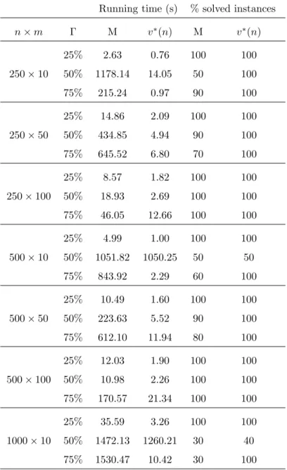
The problem Q0(y, Γ) was solved with CPLEX 11.2. For each (n, m), ten
instances have been generated. Table 1shows results of average running time
and percentage of solved instances, for each one of the two bounds previously
mentioned (see Section 3), such that the computation was stopped after 35
minutes.
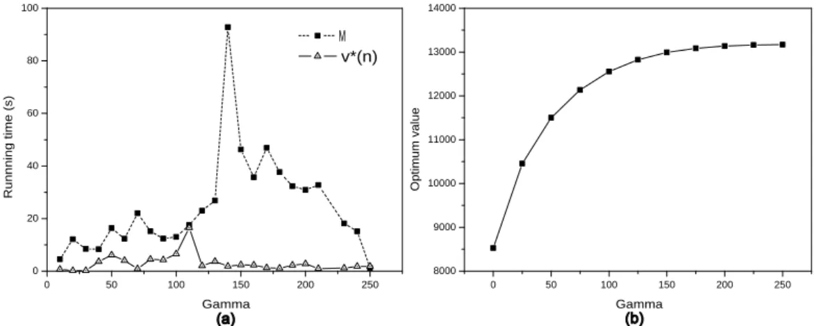
The results described in Table 1 show that the computing time obtained
by setting M to the bound v∗(n) is significantly lower than the arbitrarily
bound. Moreover, we remark that the running time increases for the value
of Γ between n/2 and n whatever the bound is (see figure 1.a). Figure 1.b
illustrates the evolution of the objective value versus Γ for a sample m = 100 and n = 250. The curve obtained is an increasing concave function, where
Table 1 Running time results
Running time (s) % solved instances
n × m Γ M v∗(n) M v∗(n) 25% 2.63 0.76 100 100 250 × 10 50% 1178.14 14.05 50 100 75% 215.24 0.97 90 100 25% 14.86 2.09 100 100 250 × 50 50% 434.85 4.94 90 100 75% 645.52 6.80 70 100 25% 8.57 1.82 100 100 250 × 100 50% 18.93 2.69 100 100 75% 46.05 12.66 100 100 25% 4.99 1.00 100 100 500 × 10 50% 1051.82 1050.25 50 50 75% 843.92 2.29 60 100 25% 10.49 1.60 100 100 500 × 50 50% 223.63 5.52 90 100 75% 612.10 11.94 80 100 25% 12.03 1.90 100 100 500 × 100 50% 10.98 2.26 100 100 75% 170.57 21.34 100 100 25% 35.59 3.26 100 100 1000 × 10 50% 1472.13 1260.21 30 40 75% 1530.47 10.42 30 100
Z(Q0(y, Γ)) increases quickly for small values of Γ and slowly for high values.
This is due to the model itself, since whenever Γ increases, the most influent uncertain parameters will be chosen.
transporta-0 50 100 150 200 250 0 20 40 60 80 100 M v*(n) Runnning time (s) Gamma 0 50 100 150 200 250 8000 9000 10000 11000 12000 13000 14000 Optimum value Gamma
Fig. 1. A sample m=100 and n=250: a. Running time vs Gamma. b. Optimal value vs Gamma
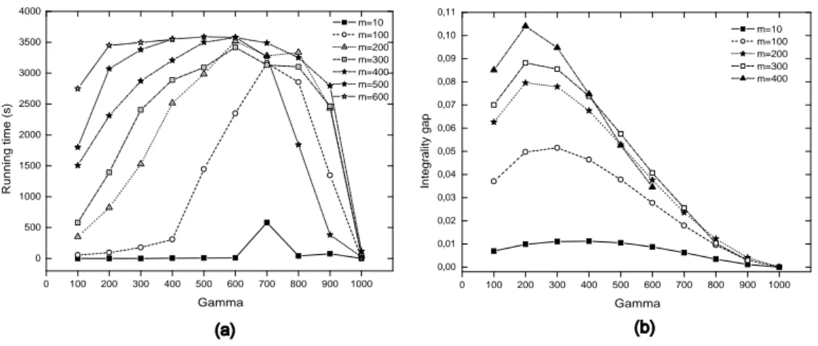
tion problem using the bound v∗(n), in order to determine the limit size of the
problem that can be solved within one hour of CPU time. Figure 2.a shows
the numerical results for a number of the uncertain demands set to n = 500. We observe that the running time grows as the number of sources m increases. Indeed, for m = 10 the problem takes few seconds to be solved. An average of 20 minutes is needed for instances with m = 80 and Γ = 60% of total deviation, and one hour for those with m ∈ [300, 500] and Γ = 50%.
0 100 200 300 400 500 0,00 0,01 0,02 0,03 0,04 0,05 0,06 0,07 0,08 0,09 0,10 0,11 0,12 0,13 0,14 0,15 Integrality gap Gamma m=10 m=20 m=30 m=40 m=50 m=60 m=70 m=80 m=90 m=100 m=200 m=300 m=400 0 100 200 300 400 500 600 0 500 1000 1500 2000 2500 3000 Running time (s) Gamma m=10 m=20 m=30 m=40 m=50 m=60 m=70 m=80 m=90 m=100 m=200 m=300 m=400
Fig. 2. Tests n=500 : a. Running time vs Gamma. b. Integrality gap vs Gamma.
demands, all instances containing m = 10 sources are solved within one hour, whatever is Γ between 10% and 100%. For 100 ≤ m ≤ 500 the solver is not able to reach the optimum within this time for Γ = 50%, and for m ≥ 600 there are memory issues with the solver.
0 100 200 300 400 500 600 700 800 900 1000 0 500 1000 1500 2000 2500 3000 3500 4000 Running time (s) Gamma m=10 m=100 m=200 m=300 m=400 m=500 m=600 0 100 200 300 400 500 600 700 800 900 1000 0,00 0,01 0,02 0,03 0,04 0,05 0,06 0,07 0,08 0,09 0,10 0,11 Integrality gap Gamma m=10 m=100 m=200 m=300 m=400
Fig. 3. Tests n=1000 : a. Running time vs Gamma. b. Integrality gap vs Gamma.
Finally, as is a very tight bound, one wants to know the behavior of the
relaxation of the mixed-integer program. Figure 2.b and Figure 3.b show the
integrality gap for the instances corresponding to n = 500 and n = 1000 demands respectively. We remark that this ratio is increasing as the number of sources m grows, reaching its maximum when Γ is around 20% of total deviation. Furthermore, the extra cost generated by the linear relaxation varies between 0 and 13% (comparing with the exact solution). For instance, if the decision maker is interested to know the worst optimal value for 70% of the total deviation from the nominal problem (which represents the most difficult instances), one can solve the linear relaxation in few secondes and have only 3% of extra cost at most. This represents a considerable saving of time.
5
Conclusion
The aim of this paper is to solve the recourse problem of the robust 2-stage location transportation problem. Previously, the 2-stage formulation has
instances with Kelley’s algorithm, was performed for about 30 uncertain pa-rameters. Here, we present the first (to our knowledge) extensive computation analysis on a particular recourse problem (namely, the location transportation problem), which is the most difficult part of the 2-stage robust optimization. Indeed, the tight bound we propose allows us to solve big size instances. Fur-thermore, this work seems to be promising to solve big size problems of the general 2-stage robust location transportation problem. This will be the aim of future research.
References
[1] A. Atamt¨urk and M. Zhang. Two-stage robust network flow and design under demand uncertainty. Operations Research, 55(4):662 – 673, 2007.
[2] A. Ben-Tal, A. Goryashko, E. Guslitzer, and A. Nimerovski. Adjustable robust solutions of uncertain linear programs. Math. Program. Ser., 99:351–376, August 2004.
[3] D. Bertsimas and M. Sim. Robust discrete optimization and network flows. Mathematical Programming Series B., 98:49–71, 2003.
[4] D. Bertsimas and M. Sim. The price of robustness. Oper. Res., 52(1):35–53, 2004.
[5] J. M. Bloemhof-Ruwaard and E. M. T. Hendrix. Generalized bilinear programming: An application in farm management. European Journal Of Operational Research, 90:102–114, 1996.
[6] J. E. Falk. A linear max-min problem. Mathematical Programming, 5:169–188, 1973.
[7] C. Floudas and P.M. Parlados. State of the Art in Global Optimization, chapter Global Optimization of separable concave functions under Linear Constraints with Totally Unimodular Matices. Kluwer, Dordrecht- Boston- London, 1995. [8] V. Gabrel and C. Murat. Duality and robustness in linear programming. to
appear in Journal of the Operational Research Society.
[9] F. Glover and E. Woolsey. Converting the 0-1 polynomial programming problem to a 0-1 linear program. Oper. Res., 22:180–182, 1974.
[10] M. Inuiguchi and M. Sakawa. Minmax regret solution to linear programming problems with an interval objective function. Eupoean Journal Of Operational Research, 86:526–536, 1995.
[11] J. E. Kelley. The cutting-plane method for solving convex programs. Society for Industrial and Applied Mathematics, 8(4):703–712, 1960.
[12] H. Konno. A cutting plane algorithm solving bilinear programs. Mathematical Programming, 11:14–27, 1976.
[13] P. Kouvelis and G. Yu. Robust discrete optimization and its applications. Kluwer Academic Publishers, 1997.
[14] HE. Mausser and M. Laguna. A new mixed integer formulation for the maximum regret problem. Int Trans Opl Res, 5(5):398–403, 1998.
[15] HE. Mausser and M. Laguna. A heuristic to minmax absolute regret for linear programs with interval objective function coefficents. European Journa of Operational Research, 117:157–174, 1999.
[16] Horst R. and H. Tuy. Global Optimization: deterministic Approaches, chapter Special Problems of Concave Minimization. Springer-Verlag Berlin Heidelberg New York, 1996.
[17] H. D. Sherali and C.M. Shetty. A finitely convergent algorithm for bilinear programming problems using polar cuts and disjunctive face cuts. Mathematical Programming, 19:14–31, 1980.
[18] A. L. Soyster. Convex programming with set-inclusive constraints and applications to inexact linear programming. Operations research, 21(5):1154– 1157, October 1973.
[19] A. Thiele, T. Terry, and M. Epelman. Robust linear optimization with recourse. Technical report, 2009.
[20] S.A. Vavasis. Nonlinear optimization, complexity issues. Oxford University Press, Oxford.