HAL Id: tel-01284113
https://hal.inria.fr/tel-01284113v2
Submitted on 29 Mar 2016
HAL is a multi-disciplinary open access
archive for the deposit and dissemination of sci-entific research documents, whether they are pub-lished or not. The documents may come from teaching and research institutions in France or abroad, or from public or private research centers.
L’archive ouverte pluridisciplinaire HAL, est destinée au dépôt et à la diffusion de documents scientifiques de niveau recherche, publiés ou non, émanant des établissements d’enseignement et de recherche français ou étrangers, des laboratoires publics ou privés.
three-dimensional moving mesh problems
Nicolas Barral
To cite this version:
Nicolas Barral. Time-accurate anisotropic mesh adaptation for three-dimensional moving mesh prob-lems. General Mathematics [math.GM]. Université Pierre et Marie Curie - Paris VI, 2015. English. �NNT : 2015PA066476�. �tel-01284113v2�
THESE DE DOCTORAT DE
L’UNIVERSITE PIERRE ET MARIE CURIE
Sp´
ecialit´
e: MATHEMATIQUES APPLIQUEES
Ecole Doctorale de Math´ematiques de Paris Centre - ED 386
Pr´esent´ee par
Nicolas Barral
Pour obtenir le grade de
Docteur de l’Universit´e Pierre et Marie Curie
Time-accurate anisotropic mesh adaptation for
three-dimensional moving mesh problems
soutenue le 27 Novembre 2015
devant le jury compos´e de:
Rapporteurs : Prof. Jean-Francois Remacle - Universit´e Catholique de Louvain Dr. Michel Visonneau - CNRS - Ecole Centrale de Nantes Directeur de th`ese : Dr. Fr´ed´eric Alauzet - INRIA Rocquencourt
Examinateurs : Prof. Thierry Coupez - Ecole Centrale de Nantes Dr. Alain Dervieux - INRIA Sophia-Antipolis Dr. Miguel ´A. Fern´andez - INRIA / UPMC Paris VI Dr. Paul Louis George - INRIA Rocquencourt Prof. David L. Marcum - Mississippi State University
Remerciements
Je tiens `a remercier tout d’abord Fr´ed´eric Alauzet, mon directeur de th`ese, qui m’a donn´e la possibilit´e de d´ecouvrir le monde de la recherche en me proposant ce sujet. Je lui suis tr`es reconnaissant de m’avoir fait partager son savoir et son exp´erience avec patience et disponibilit´e. Je suis particuli`erement reconnaissant envers Paul Louis George, responsable du projet Gamma, pour son encadrement strict mais juste d`es mon arriv´ee dans le projet, et pour m’avoir patiemment transmis une petite part de son savoir (qui est grand...).
Je suis tr`es honor´e que Messieurs Jean-Fran¸cois Remacle et Michel Visonneau aient accept´e de rapporter mon travail et je les en remercie. Je suis ´egalement reconnaissant envers Messieurs Thierry Coupez, Alain Dervieux, Miguel Fern´andez, Paul Louis George et Dave Marcum pour leur participation `a mon jury.
Un grand merci `a tous les membres du projet Gamma que je vois tous les jours depuis cinq ans, pour les discussions int´eressantes avec certains, et les bons moments de d´etente avec d’autres, les deux ensembles n’´etant pas d’intersection nulle: Adrien - qui m´eriterait une phrase `
a lui tout seul si mon r´epertoire de synonymes ´etait plus ´eto↵´e-, Lo¨ıc, Dave, Houman, Patrick, Victorien, Alexis, Olivier, Lo¨ıc sans oublier Maryse pour son aide pr´ecieuse. Mention sp´eciale `a Julien, Alex et Eleonore, pour m’avoir support´e dans le mˆeme bureau. Merci aussi `a St´ephanie, Bruno et Estelle, ainsi qu’`a G´eraldine, sans son travail approfondi cette th`ese n’aurait pas ´et´e bien loin. Mes remerciements `a tous les gens des autres ´equipes et bˆatiments crois´es plus ou moins longuement ici et l`a.
Je remercie mes amis, qui auront support´e mes sautes d’humeur et que j’ai parfois injuste-ment n´eglig´es, Antoine, Camille, C´edric, Jeanne, Lindsay, Ma¨ıssane, Marion, M´elanie, Nicolas, Paco, Sibylle, tous ceux d’IRC, Dominique, Benjamin, Florence, Cyprien, Fabien, Valentin, sans oublier tous ceux que j’oublie et qui ne m’en voudront pas.
Je voudrais ´egalement remercier la Principaut´e de Monaco, et la Direction de l’Education Nationale, de la Jeunesse et des Sports, pour leur soutien.
Enfin, je veux remercier ma famille pour son soutien sans faille tout au long de la th`ese, malgr´e les ´epreuves douloureuses qu’elle traverse, `a cˆot´e desquelles la convergence d’un r´esidu ou la r´ejection d’un papier sont bien peu de choses.
Contents
Conventions 3
Introduction 5
I 3D FSI moving mesh simulations 11
Introduction 13
1 Connectivity-change moving mesh strategy 15
1.1 Our moving mesh algorithm . . . 17
1.1.1 A two step process . . . 17
1.1.2 Mesh deformation step . . . 17
1.1.3 Mesh optimization step . . . 20
1.1.4 Optimization procedure . . . 22
1.1.5 Handling of boundaries . . . 23
1.1.6 Algorithm . . . 23
1.1.7 Choice of the di↵erent parameters for a robust algorithm . . . 23
1.2 Mesh deformation with Inverse Distance Weighted method. . . 25
1.2.1 IDW method . . . 25
1.2.2 Implementation . . . 27
1.3 Examples . . . 28
1.3.1 Rigid-body examples . . . 28
1.3.2 Deformable-body examples . . . 32
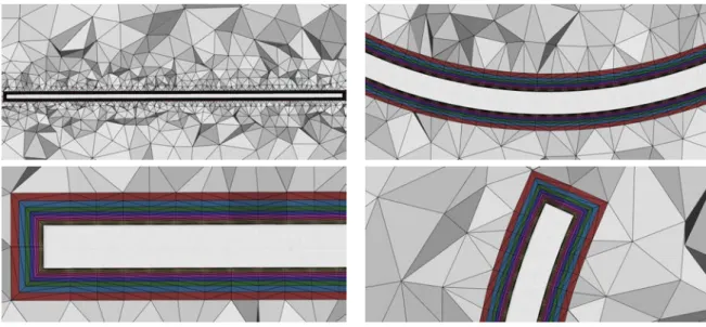
1.4 Boundary layers for deformable geometries. . . 36
1.4.1 One boundary layer . . . 39
1.4.2 Several boundary layers . . . 40
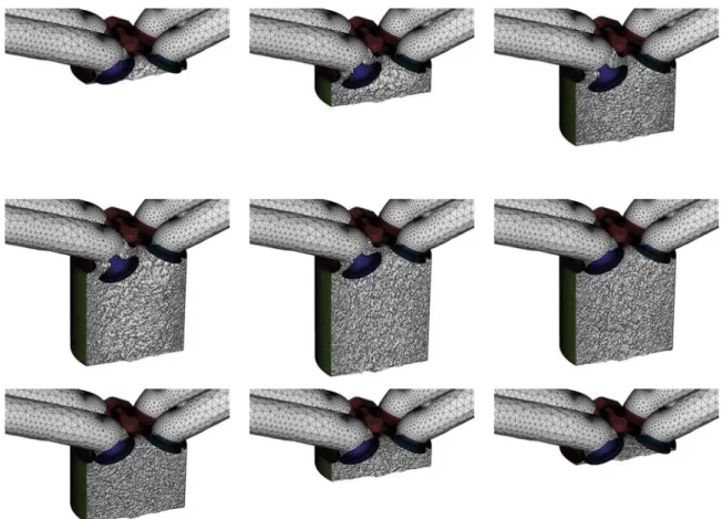
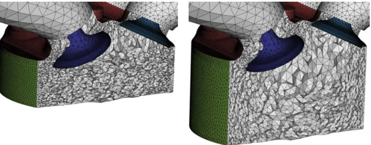
1.5 Large volume variations . . . 40
1.5.1 Engine piston . . . 41
1.6 Conclusion . . . 44
2 ALE solver 47 2.1 Euler equations in the ALE framework . . . 47
2.2 Spatial discretization . . . 47
2.2.1 Edge-based Finite-Volume solver . . . 48
2.2.2 HLLC numerical flux. . . 48
2.2.3 High-order scheme . . . 49
2.2.4 Limiter . . . 50
2.2.5 Boundary conditions . . . 51
2.3.1 The Geometric Conservation Law. . . 52
2.3.2 Discrete GCL enforcement. . . 52
2.3.3 RK schemes . . . 53
2.3.4 Application to the SSPRK(4,3) scheme . . . 53
2.3.5 Practical computation of the volumes swept . . . 55
2.3.6 MUSCL approach and RK schemes . . . 58
2.3.7 Computation of the time step . . . 58
2.3.8 Handling the swaps . . . 58
2.4 FSI coupling . . . 59
2.4.1 Movement of the geometries . . . 59
2.4.2 Discretization . . . 60 2.4.3 Explicit coupling . . . 60 2.5 Implementation . . . 60 2.5.1 Non-dimensionalization . . . 60 2.5.2 Parallelization . . . 60 2.6 Conclusion . . . 61 3 Numerical Examples 63 3.1 Validation of the solver . . . 63
3.1.1 Static vortex in a rotating mesh . . . 63
3.1.2 Flat plate in free fall . . . 67
3.1.3 Piston . . . 69
3.2 Numerical examples . . . 72
3.2.1 AGARD test cases . . . 72
3.2.2 F117 nosing up . . . 76
3.2.3 Two F117 aircraft crossing flight paths. . . 79
3.2.4 Ejected cabin door . . . 82
3.3 Parallel performance . . . 83
3.4 Conclusion . . . 84
Conclusion 84 II Extension of anisotropic metric-based mesh adaptation to moving mesh simulations 89 Introduction 91 4 Basics of metric based mesh adaptation 95 4.1 State of the art . . . 95
4.1.1 Meshing status . . . 95
4.1.2 History of metric-based mesh adaptation. . . 96
4.1.3 Other mesh adaptation approaches . . . 98
4.2 Principle of metric-based adaptation . . . 98
Contents v
4.2.2 Unit mesh . . . 102
4.2.3 Operations on metrics . . . 103
4.2.4 The non-linear adaptation loop . . . 106
4.3 The continuous mesh framework . . . 111
4.3.1 Duality discrete-continous: a new formalism . . . 111
4.3.2 Continuous linear interpolation . . . 113
4.3.3 Summary . . . 115
4.4 Multiscale mesh adaptation . . . 116
4.4.1 Optimal control of the interpolation error and optimal meshes . . . 116
4.4.2 Control of the error in Lp norm . . . 119
4.5 Conclusion . . . 119
5 Unsteady mesh adaptation 121 5.1 Error estimate . . . 122
5.1.1 Error model . . . 122
5.1.2 Spatial minimization for a fixed t . . . 123
5.1.3 Temporal minimization . . . 123
5.1.4 Error analysis for time sub-intervals . . . 124
5.1.5 Global fixed-point mesh adaptation algorithm . . . 126
5.2 From theory to practice . . . 127
5.2.1 Computation of the mean Hessian-metric . . . 127
5.2.2 Choice of the optimal continuous mesh. . . 129
5.2.3 Matrix-free P1-exact conservative solution transfer . . . 129
5.2.4 The remeshing step . . . 130
5.2.5 Software used . . . 130
5.3 Choice of the mean Hessian-metric . . . 130
5.4 Numerical examples . . . 140
5.4.1 2D shock-bubble interaction . . . 140
5.4.2 3D circular blast . . . 142
5.4.3 3D shock-bubble interaction . . . 145
5.4.4 3D blast on the London Tower Bridge . . . 148
5.5 Parallelization of the mesh adaptation loop . . . 149
5.5.1 Choices of implementation. . . 149
5.5.2 Analysis of parallel timings . . . 153
5.5.3 Conclusion . . . 155
5.6 Conclusion . . . 156
6 Extension of unsteady adaptation to moving meshes 157 6.1 ALE metric . . . 158
6.2 Analytic examples . . . 159
6.2.1 Procedure . . . 159
6.2.2 Functions considered . . . 161
6.2.3 Results . . . 164
6.3.1 Error analysis . . . 176
6.3.2 Algorithm . . . 177
6.3.3 Update of the metric for optimizations . . . 178
6.3.4 Handling of the surface . . . 179
6.4 3D numerical examples. . . 179
6.4.1 Shock tube in expansion . . . 179
6.4.2 Moving ball in a shock tube . . . 180
6.4.3 Nosing-up f117 . . . 183
6.4.4 Two F117 aircraft flight paths crossing. . . 183
6.5 Conclusion . . . 183
Conclusion 184 Conclusion and perspectives 188 Acknowledgments 191 Appendices 193 A Intersection of metrics 197 A.1 In two dimensions . . . 197
A.2 In three dimensions. . . 198
B GPU acceleration of a 3D Finite Volume flow solver 201 B.1 Solver used . . . 201
B.2 GPU acceleration . . . 202
B.3 State of the art . . . 203
B.4 Principles of implementation . . . 204
B.5 Results and timings . . . 206
B.6 Conclusion . . . 211
R´
esum´
e
Les simulations d´ependant du temps sont devenues une n´ecessit´e pour l’industrie, et notamment celles mettant en oeuvre des g´eom´etries mobiles, avec mouvement impos´e ou avec des interac-tions de type fluide-structures. Toutefois, de nombreuses difficult´es subsistent qui empˆechent d’e↵ectuer de telles simulations de mani`ere quotidienne `a une pr´ecision acceptable. Parmi ces difficult´es, les g´eom´etries mobiles, en particulier celles pr´esentant des grands d´eplacements, ne sont en g´en´eral pas trait´ees de fa¸con satisfaisante, aussi bien du point de vue du temps de calcul que de la pr´ecision des algorithmes. L’adaptation de maillage anisotropes bas´ee sur les m´etriques a prouv´e son efficacit´e pour am´eliorer la pr´ecision des calculs stationnaires pour un coˆut en temps maˆıtris´e. Mais son extension aux probl`emes d´ependant du temps est loin d’ˆetre ´evidente, et l’ajout de g´eom´etries mobiles complique encore plus le probl`eme. Dans cette th`ese, on s’int´eresse `a divers ´el´ements des simulations instationnaires en g´eom´etrie mobile, avec l’objectif global de les rendre automatiques et d’en am´eliorer les performances. Dans la continuit´e de [Olivier 2011a], des contributions sont apport´ees `a tous les ´el´ements de la chaˆıne, algorithme de bouger de maillage, solveur Arbitrairement Langrangien Eulerien (ALE) et adap-tation insadap-tationnaire, conduisant `a la mise au point d’un algorithme d’adaptation de maillage pour des simulations en g´eom´etrie mobile.
On consid`ere un algorithme de bouger de maillage fond´e sur des changements de connectivit´e (swaps) pour pr´eserver la qualit´e du maillage. Une nouvelle m´ethode de calcul de la d´eformation du maillage, par interpolation directe (m´ethode IDW), a ´et´e ajout´ee, et compar´ee `a la m´ethode pr´eexistante par r´esolution d’une EDP d’´elasticit´e lin´eaire. Ces deux m´ethodes pr´esentent toutes deux des performances excellentes, ce qui prouve la robustesse de l’algorithme pour g´erer des maillages mobiles sans remaillage global, y compris avec de grands d´eplacements. Dans cette th`ese, on aborde ´egalement les corps d´eformables avec des couches limites ou des grandes variations de volume.
Cet algorithme de bouger de maillage a ´et´e con¸cu pour ˆetre utilis´e avec un solveur ALE, que l’on pr´esente en d´etail. Une discr´etisation par Volumes Finis est e↵ectu´ee, avec un solveur de Riemann approch´e de type HLLC, et une reconstruction des gradients de type MUSCL pour obtenir un ordre 2 en espace. La discr´etisation en temps repose sur une analyse fine de la Loi de Conservation G´eom´etrique (GCL), qui permet de construire des sch´emas de Runge-Kutta `a plusieurs pas d’ordres ´elev´es. Le calcul de certaines quantit´es g´eom´etriques en trois dimensions est clarifi´e. Les changements de connectivit´e du maillage sont trait´es par une interpolation lin´eaire entre deux pas de temps du solveur.
Ce solveur a ´et´e impl´ement´e en trois dimensions, parall´elis´e et valid´e sur plusieurs cas. Ces derniers ont confirm´e les ordres de convergence attendus. En particulier, l’influence des swaps a ´et´e ´etudi´ee, et il en d´ecoule que le faible nombre de ces op´erations rend leur influence n´egligeable sur la convergence et la pr´ecision des solutions. D’autres exemples tri-dimensionnels sont pr´esent´es dans le champ de la M´ecanique des Fluides Num´erique (CFD), plus complexes en terme de flux ´etudi´es, de g´eom´etries et de d´eplacements des g´eom´etries, avec des d´eplacements impos´es ou d´erivant d’un couplage Fluide-Structure. Ils prouvent l’efficacit´e de l’approche retenue, qui permet de simuler des probl`emes en maillage mobile complexes dans un temps
raisonnable sans jamais remailler globalement.
Des progr`es ont ´et´e r´ealis´es depuis le premier algorithme d’adaptation instationnaire de point fixe dans [Alauzet 2003a]. Dans cette th`ese, une nouvelle version de l’algorithme de point fixe est utilis´ee, fond´ee sur une nouvelle analyse de l’erreur espace-temps dans le cadre de la th´eorie du maillage continu. Th´eorie et exp´erimentation ont permis de clarifier et valider certains points cruciaux du processus, notament le choix d’une Hessienne moyenn´ee essentielle `a l’algorithme. Grˆace `a une parall´elisation efficace de type p-threads, dont on fournit une analyse, plusieurs cas d’adaptation instationnaire en 3D ont ´et´e simul´es avec une pr´ecision difficilement concevable il y a encore quelques ann´ees.
Finalement, toutes ces briques ont ´et´e assembl´ees pour conduire `a un algorithme d’adaptation pour simuler des ph´enom`enes physiques instationnaires en maillage mobile utilisant l’algorithme de bouger de maillage avec changements de connectivit´e. La m´etrique ALE qui avait ´et´e pr´esent´ee dans [Olivier 2011a] et permettait de bouger un maillage en un maillage adapt´e est int´egr´ee `a une analyse d’erreur fond´ee sur l’approche du maillage continu. Cela conduit `a une correction de la m´etrique optimale dans l’algorithme de point fixe. En plus de l’utilisation de cette nouvelle m´etrique, d’autres ajouts ont ´et´e e↵ecut´es par rapport `a l’algorithme standard pour utiliser des maillages mobiles. En particulier la m´etrique sur laquelle les optimisations de maillage de l’algorithme de bouger sont e↵ectu´ees est modifi´ee. Finalement, plusieurs exem-ples sont pr´esent´es, qui confirment que l’adaptation de maillage anisotrope permet un gain de pr´ecision en un temps raisonnable pour les simulations en maillage mobile complexes.
Conventions
Simplicial mesh
Let n be the dimension of the physical space and let ⌦ ⇢ Rn be the non-discretized physical domain. ⌦ is an affine space. The canonical basis of its vectorial space is noted (e1, e2, . . . , en) in general, but notations (ex, ey) and (ex, ey, ez) can also be used in two and three dimensions. Vectors ofRn are noted in bold font. The coordinate vector of a point of ⌦ is generally noted x = (x1, . . . , xn).
The boundary of ⌦, noted @⌦, is discretized using simplicial elements the vertices of which are located on @⌦. In two dimensions, @⌦ is discretized with segments while in three dimensions, boundary surfaces @⌦ are represented by triangles. The discretized boundary is noted @⌦h and ⌦h denotes the sub-domain ofRn having @⌦h as boundary.
Building a mesh of ⌦h consists in finding a set of simplicial elements - triangles in two dimensions, tetrahedra in three dimensions - notedH, satisfying the following properties:
• Non-degenerescence: Each simplicial element K of H is non-degenerated (no flat elements of null area or volume),
• Covering: ⌦h = [ K2 H
K ,
• Non-overlapping: The intersection of the interior of two di↵erent elements of H is empty: ˚
Ki\ ˚Kj =?, 8 Ki, Kj 2 H, i 6= j .
• Conformity: The intersection of two elements is either a vertex, an edge or a face (in three dimensions) or is empty.
The conformity hypothesis is adopted here, because the meshes will be used with a Finite-Volume solver which requires the enforcement of this constraint. Besides, it facilitates the handling of data structures on the solver side and also enables to save a consequent amount of CPU time.
Finally, a mesh is said to be uniform if all its elements are almost regular (equilateral) and have the same size h.
Notations and orientation conventions
The following notations will be used in this thesis: K is an element of the mesh H, Pi is the vertex ofH having i as global index, eij is the edge linking Pi to Pj. The number of elements, vertices and edges are noted Nt, Nv and Ne, respectively.
The vertices and the edges of an element K are also numbered locally. Vertex numbering inside each element is done in a counter-clockwise (or trigonometric) manner, which enables
to compute edges/faces outward normals in a systematic way. This numbering, as well as unit outward normals n and edges/faces orientations are shown for triangles and tetrahedra in Figure 1. Non-normalized normals will be noted ⌘.
P0 P1 P2 P3 e0 e1 e2 e3 e4 e5 P0 P1 P2 P3 n0 n1 n2 n3 P0 P1 P2 P3 P0 P1 P2 P0 P1 P2 P0 P1 P2 e0 e1 e2 n0 n1 n2
Figure 1: Conventions in a simplicial element K in two (top) and three (bottom) dimensions. Conventions for vertex numbering, edge numbering and orientation (left), unit normal number-ing and orientation (middle) and face(s) orientation (right).
Introduction
In 1953, the first civil numerical simulation, also know as Fermi-Pasta-Ulam-Tsingou experi-ment, focused on a unidimensional system with 64 masses coupled with springs (i.e. 64 vertices). In sixty years, numerical simulation has come a long way, together with the development of com-puting resources. As it became possible to model and simulate more complex problems, industry started to take advantage of its potentialities. In particular, the aeronautic industry quickly saw a way to avoid costly full-size experiments, and has, together with military applications, been a driving force in the development of numerical simulation.
Nowadays, computers with hundreds of thousands of cores are available, and sophisticated numerical models enable running complex multiphysics simulations, involving fluid mechanics, structural mechanics, thermodynamics and electromagnetism. Most of the fields of scientific research resort to numerical simulation, from physics to social sciences through engineering and medicine, with more or less success. However, as the simulation capabilities grow, so do the requirements of both industries and researchers, and a whole set of problems have arisen. Notably, the increase in computational power allows scientists to not content themselves with steady approximations of the physical phenomena, and to study the e↵ects of time-dependent parameters.
In this thesis, we focus on Computational Fluid Dynamics (CFD), i.e. the science of simu-lating numerically fluid flows, and its applications to aeronautic, although the results presented can be used in a vast field of research and industry. The theme of this thesis is unsteady simu-lations, and in particular simulations with moving boundaries. This subject is tackled from the points of view of meshes and mesh adaptation.
Problem
Most real-life phenomena are unsteady, but scientists are still far from running simulations close to real life on a daily basis. Problems arising from unsteady simulations are of multiple kind. To be used by industry, the results of numerical simulations have to be trusted, and the certification of the accuracy of the solutions is harder than for steady problems. Instabilities impact more the solution, and it is difficult to control the error in time at long temporal scales. Unsteady simulations are intrinsically longer than steady simulations, due to restrictions on the solvers time steps, and it is all the more difficult to control the error over time at a reasonable CPU time cost. Solutions to efficiency issues have to be found. Unsteady simulations often involve the interactions of one or several bodies evolving in one or several fluids, which require considering Fluid-Structure Interaction coupling techniques. Very often, moving boundaries have to be dealt with, which is often done by moving the mesh. This proves to be complex, especially for large displacements and in three dimensions, where meshing techniques are still evolving.
State of the art
Mesh adaptation has proved over the past twenty-five years its ability to increase signif-icantly the accuracy of numerical simulations for a reasonable CPU time cost. A large number of di↵erent approaches have been considered, for various applications, from aero-dynamics to biomechanics and magnetoaero-dynamics. Metric-based mesh adaptation has no-tably resulted in considerable gain in terms of accuracy and CPU time for steady prob-lems [Hecht 1997,Bottasso 2004,Gruau 2005,Loseille 2010a,Gu´egan 2010]. A first attempt at extending it to unsteady simulations was carried out in [Alauzet 2003a], which was promising. This work was carried on in [Olivier 2011a], in which more solid theoretic bases were brought to support the method, and in which metric-based mesh adaptation was used for the first time on two dimensional moving meshes.
Objective
The works presented in this thesis follow on from [Olivier 2011a]. I focused on two aspects of mesh adaptation for moving mesh problems: on the one hand, the handling of moving meshes themselves, and on the other hand metric based mesh adaptation for unsteady simula-tions. First, I aimed at improving the strategy for simulations with moving meshes developed in [Olivier 2011a,Alauzet 2014a], based on a connectivity-change moving mesh algorithm cou-pled to an ALE solver. Variants to the algorithm needed to be considered, as well as the implementation and validation of the solver in 3D. Regarding unsteady simulations, the objec-tive was to integrate the latest theoretic updates to the adaptation algorithm, both for fixed and moving meshes, and to extend to 3D the work of [Olivier 2011a] on adaptation for moving meshes.
Numerical context
The present work was conducted in the GAMMA3 research group at INRIA. Most numerical choices naturally stem from those made in the group, to benefit from both the considerable experience and the valuable software of its members.
We consider unstructured meshes, i.e. meshes made up of triangles (in 2D) or tetrahedra (in 3D). This is due to the fact that it is easier to mesh complex geometries with simplexes, resulting in several fully automatic unstructured three-dimensional meshing codes, and to the flexibility of such elements enabling anisotropic mesh adaptations.
Anisotropic metric-based mesh adaptation techniques are considered, which present several advantages compared to other adaptation techniques. First, it allows us to handle anisotropic meshes, which are of great value in mesh adaptation because they enable a more optimal dis-tribution of the mesh vertices, and because the orientation of the elements is accorded to the physical phenomena at stake. Moreover, the theory of metric-based adaptation is well estab-lished, and several research groups contribute to its development. In particular, the recent advent of the continuous mesh framework [Loseille 2011a, Loseille 2011b] was a major break-through in this field, opening the way to a more rigorous analysis of error optimization problems. Finally, several research works establish the ability of metric-based mesh adaptation to handle complex steady simulations in three dimensions, which is promising for unsteady problems.
Contents 7 Regarding moving-boundary meshes, the body-fitted approach has been preferred to im-mersed boundaries and Chimera (overset) methods. We consider a unique body-fitted mesh, that follows the moving geometry in time, because it enables an accurate treatment of bound-aries, unlike immersed boundaries methods where the boundary is not explicitly meshed, and because there is no interpolation step unlike Chimera methods where the solutions on the dif-ferent sub-grids have to be transferred to one another, resulting in spoiling interpolation error. From the solver point of view, the classic Arbitrary-Lagrangian-Eulerian (ALE) framework is used, that enables writing the physical equations on a mesh moving with an arbitrary movement. Finally, application examples have been chosen in the field of CFD, and only mono-fluid problems modeled by the inviscid compressible Euler equations are considered. Driven by industrial concern, most of the simulations are three dimensional.
Main contributions
During this thesis, I updated the existing algorithms both for moving mesh handling and for unsteady mesh adaptation. I implemented these updates and tested them on a wide variety of test cases. Notably, I extended the previous works of [Olivier 2011a] to 3D.
• I added a new mesh deformation method (the Inverse Distance Weighted (IDW) method) to our moving mesh code, and compared it to the elasticity-like method already implemented. • I partially implemented and parallelized the ALE solver from [Olivier 2011a] in 3D, validated it on academic test cases and ran complex 3D ALE simulation both with imposed motion and FSI.
• I updated the unsteady adaptation algorithm with the latest theoretical results, using the continuous mesh framework to derive a better expression for the averaged ”Hessian-metric”, and ran 3D simulations of unprecedented size thanks to an efficient parallelization of the algorithm.
• I updated the error analysis from [Olivier 2011a] for adaptative moving mesh problems, implemented the resulting algorithm, and ran several 3D adaptive simulations with moving boundaries.
Outline
This thesis is structured in two parts, that cover the two aspects of adaptation for moving mesh problems.
In the first part (Part I), aspects linked to the moving mesh computations are considered. First, we focus on the moving mesh strategy used in the whole thesis, describing every aspects of the algorithm, and analyzing the performance of updates to this algorithm. It is notably based on mesh connectivity changes (edge/face swaps), to preserve the quality of the mesh throughout large displacements without remeshing. This algorithm was designed to run ALE simulations on the moving meshes, and an ALE solver was actually implemented in 3D. It is described in details, from the formulation of the equations and the choices of numerical methods to implementation and parallelization considerations. Validation examples of the solver are presented, followed by
more complex CFD cases coupling the ALE solver and the connectivity-change moving mesh algorithm, proving the efficiency of the approach in 3D.
The second part (Part II) deals with mesh adaptation, from the basics of metric-based adaptation to adaptation with moving meshes, through unsteady simulation on fixed meshes. All the theoretical background necessary for the rest of the part is recalled, notably the continuous mesh framework and multiscale mesh adaptation. The continuous mesh framework enabled a new analysis of the space-time error for unsteady simulations, which is presented, and leads to a new version of the unsteady adaptation algorithm. Practical aspects of the implementation of this algorithm are reviewed, and new 3D examples are given. This algorithm is extended to moving meshes: the ALE metric introduced in [Olivier 2011a] is plugged into the unsteady error analysis, and the resulting adaptation algorithm is described. Finally, examples of 3D adaptative simulations with moving mesh are exhibited, that validate the whole approach followed in this thesis.
Scientific communications
Journal articles
• Three-dimensional large displacement CFD simulations using a connectivity-change moving mesh approach, N. Barral and F. Alauzet, Journal of Computational Physics, submitted.
• Construction and geometric validity (positive Jacobian) of serendipity Lagrange finite elements, theory and practical guidance, P.L. George, H. Borouchaki and N. Barral, Mathematical Modelling and Numerical Analysis, submitted.
• Geometric validity (positive Jacobian) of high-order Lagrange finite elements, theory and practical guidance, P.L. George, H. Borouchaki and N. Barral, Engineering with computers, accepted.
Proceedings with peer review
• Metric-Based Anisotropic Mesh Adaptation for Three-Dimensional Time-Dependent Problems Involving Moving Geometries, N. Barral, F. Alauzet and A. Loseille, 53th AIAA Aerospace Sciences Meeting, AIAA Paper 2015-2039, Kissimmee, FL, USA, Jan 2015.
• Two mesh deformation methods coupled with a changing-connectivity moving mesh method for CFD Applications, N. Barral, E. Luke and F. Alauzet, Proc. of the 23th International Meshing Roundtable, Procedia Engineering, vol 82, pp. 213-227, London, England, 2014.
• Large displacement body-fitted FSI simulations using a mesh-connectivity-change moving mesh strategy, N. Barral and F. Alauzet, 44th AIAA Fluid Dynamics Conference, AIAA Paper 2014-2773, Atlanta, GA, USA, June 2014.
Contents 9 Communications
• Anisotropic Error Estimates for Adapted Dynamic Meshes, N. Barral and F. Alauzet, ADMOS 2015, Nantes, France, June 2015.
• Large displacement simulations with an efficient mesh-connectivity-change mov-ing mesh strategy, N. Barral and F. Alauzet, ECCOMAS 2014, Barcelona, Spain, July 2014.
• Parallel time-accurate anisotropic mesh adaptation for time-dependent prob-lems, N. Barral and F. Alauzet, ECCOMAS 2014, Barcelona, Spain, July 2014.
Research reports
• Construction et validation des ´el´ements Serendip associ´es `a un carreau de degr´e arbitraire, P.L George, H. Borouchaki and N. Barral, INRIA RR-8572, 2014.
• Construction et validation des ´el´ements r´eduits associ´es `a un carreau simplicial de degr´e arbitraire, P.L George, H. Borouchaki and N. Barral, INRIA RR-8571, 2014. Talks and seminars
• Adaptation de maillages non structur´es pour des probl`emes instationnaires, et maillage en g´eom´etrie mobile, N. Barral, Groupe de travail ”Analyse Num´erique et EDP”, Ecole Centrale Paris, November 2014.
• Du r´eel au num´erique : la science des maillages, P.L. George and N. Barral, Pint of Science, May 2015.
Awards
• IMR Meshing Contest Award, 23th International Meshing Roundtable, London, Octo-ber 2014.
Part I
Introduction
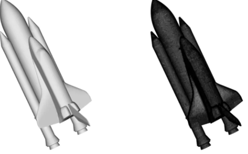
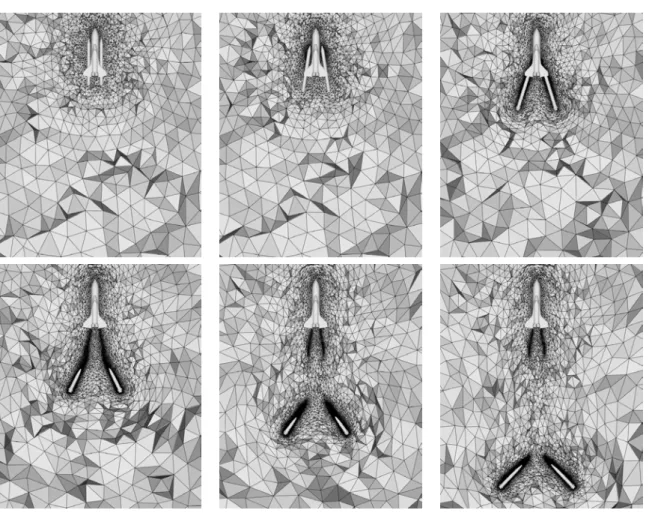
Fluid-structure interaction (FSI) simulations are required for a wide variety of subjects, from the simulation of jellyfish [Etienne 2010] to the releasing of a missile [Murman 2003,Hassan 2007], through the simulation of aortic valves [Astorino 2009], cardiovascular systems [Formaggia 2009,
Gerbeau 2014], ship propellers [Comp`ere 2010], tuning forks [Froehle 2014], wind tur-bines [Bazilevs 2011], 2D airbag deployment and balloon inflation [Saksono 2007]. Other prob-lems such as icing [Tong 2014,Pendenza 2014] or blast studies [Baum 1996] do not involve FSI but share a lot of common problems with FSI simulations. The recent development of com-puting capacities has made it possible to run increasingly complex simulations where moving bodies interact with an ambient fluid in an unsteady way. However, engineers are still far from performing such simulations on a daily basis, largely due to the difficulty of handling the moving meshes induced by the moving geometries.
When the displacement of the geometry is small enough, slightly deforming the original mesh [Batina 1990, Degand 2002] can generally be acceptable. But when large deformation of the boundaries is considered, the mesh quickly becomes distorted and the numerical error due to this distortion quickly becomes too great, until the elements of the mesh finally become invalid, and the simulation has to be stopped. Specific strategies need to be developed to deal with large displacement moving boundary problems. In the case of FSI problems, another difficulty arises from the fact that the displacement of the boundaries is by definition an unknown, and the deformation of the mesh cannot be imposed a priori. Addressing the issue of the mesh movement cannot be separated from addressing the issue of the solver that will compute on these moving meshes. Depending on the strategy employed to deal with the movement, specific numerical methods must be designed to take into account the displacement of the mesh.
The question this part focuses on is: how can we efficiently move the mesh for large dis-placement 3D FSI simulations and what numerical schemes need to be associated to such a strategy ?
Three main approaches to address the mesh movement problem can be found in the litera-ture. The first approach consists in having a single body-fitted mesh [Baum 1994,Hassan 2007], and moving it along with the moving boundaries. The mesh may thus undergoe large defor-mation. The second approach is the Chimera (or overset) method [Benek 1985], in which each moving body has its own body-fitted sub-mesh, and the sub-meshes move rigidly to-gether with their body and can overlap one another. Finally the embedded boundary ap-proach [Bruchon 2009, L¨ohner 2001] uses meshes that are not body-fitted at all: the bodies are embedded in a fixed grid, and techniques such as level-sets are used to recover their mov-ing boundaries. All three approaches have their own strengths and weaknesses. For meshmov-ing purposes and to fit our mesh adaptation context, we focus on body-fitted approaches with one single mesh. Our approach was introduced in [Alauzet 2014a] and was enhanced during this thesis.
In some works, a mesh motion that is directly adapted to the physical phenomena in question is applied, using for instance either so-called Moving Mesh PDEs [Huang 2010b] or a Monge-Amp`ere equation [Chac´on 2011]. More generally, these approaches come under the r-adaptation
category (see Section 4.1.3). However interesting these approaches may be, they still seem to be time consuming, especially in 3D, due to the solution of a non-linear equation, and it is unsure whether they can handle complex 3D geometries. Therefore we prefer to prescribe arbitrary movements to the mesh, and use our mesh adaptation framework [Loseille 2011a] when necessary, as will be detailed in Part II, Chapter 6.
As regards numerical solvers, we consider a classic framework for moving meshes: the Arbi-trary Lagrangian Eulerian (ALE) framework, which is based on a formulation of the equations that takes into account an arbitrary movement of the vertices. This technique was introduced in the 70s in [Hirt 1974,Hughes 1981,Donea 1982]. Since then, so many developments have been made in that field that a complete list of them would not fit in this thesis. However, one may in particular refer to [Nkonga 1994,Baum 1994,Farhat 2001,Formaggia 2004,Mavriplis 2006,
Hassan 2007, Hay 2014], which mainly focus on improving temporal schemes for ALE simula-tions.
To our knowledge, very few examples of ALE solvers coupled with connectivity-change moving mesh techniques can be found in the literature. In [Kucharik 2008] a conservative interpolation is proposed to handle the swaps. In [Guardone 2011, Olivier 2011b] an ALE formulation of the swap operator is built. However, these studies are limited to 2D. Driven by the requirements of industry, we are interested in designing a method that works in 3D. In this thesis, a linear interpolation is carried out after each swap instead of using a specific ALE formulation, and we will evaluate the numerical error due to these swaps.
The goal of this part is to demonstrate that three-dimensional FSI simulations with large displacement can be run efficiently by coupling an ALE solver to our connectivity-change moving mesh strategy. This part is structured as follows. In Chapter1, the moving mesh strategy used and improved during this thesis is described in detail, and analyzed on purely moving-mesh simulations. In Chapter 2, the ALE solver that was implemented in 3D during this thesis is described, from the formulation of the equations to implementation considerations. Finally Chapter 3presents a large number of moving-mesh ALE simulations, both academic test cases and more complex CFD simulations, coupling the moving mesh strategy and ALE solver.
Chapter 1
Connectivity-change moving mesh
strategy
When dealing with a unique body-fitted moving mesh, two main approaches are used.
The first one is simply to move the mesh for as long as possible, with a constant topology, and remesh when the quality becomes critical. For each remeshing, the simulation has to be stopped, a new mesh must be generated (a whole new mesh or parts of it), new data structures must be created, and the solution must be transferred to the new mesh. This approach can be efficient, especially when small displacements are considered and very few remeshings are necessary, because the solver and the meshing aspects are decoupled. Between two remeshings the simulation is fully ALE and free from interpolation errors due to con-nectivity changes. However, for larger displacements, the number of remeshings increases to prevent invalid elements from appearing, especially if shearing appears. This can be costly in terms of CPU, but also result in poor accuracy due to the numerous solution transfer steps. This strategy is for instance used in [Murman 2003] with hexaedral Cartesian meshes, or [L¨ohner 1990a,Hassan 2000,Jayaraman 2000] on unstructured meshes.
The second approach tries to preserve a good mesh quality throughout the simulation by performing local remeshing operations such as vertex insertion, vertex collapse, connectivity changes and vertex displacements. It is used for example in [Dobrzynski 2008,Comp`ere 2010]. The advantage of this method is that it maintains an acceptable mesh quality without need-ing to stop, remesh and resume the simulation. However, it requires fully dynamic mesh data structures that are permanently updated, which can lead to a loss of CPU efficiency, and the numerous mesh modifications tend to lead to a loss of accuracy due to interpolation errors.
In our case, we want to address the case of large and complex displacements of the bound-aries, with potentially highly non-linear trajectories as may occur in FSI simulations. This requires that the moving mesh strategy fulfills a number of properties:
• It must above all preserve the validity of the mesh, and never create elements with a negative volume.
• It must preserve the quality of the elements of the mesh all along the simulation, to ensure a good solution accuracy and reasonable solver time steps.
• It must be efficient in terms of CPU since the mesh must be moved at each solver iteration. It must not take for more than a small fraction of the total simulation time.
• It must be robust, and be able to deal with very small elements, and large shearing con-straints.
• It must be able to preserve the anisotropic adaptation if any.
For efficiency purposes, we add that we want to remesh as little as possible, and that most cases should be run without remeshing at all.
Remark 1. What we call remeshing entails: stopping the simulation, calling meshing software to generate either a whole new mesh or parts of it, and interpolate the solution on the new mesh. This is costly because (a) it usually requires the use of an external code, with its own data structures, requiring CPU-expensive data transfers, (b) the meshing step can be long (and might not even complete) in the case of complex geometries, (c) an interpolation step which produces not too much error is long too, especially if the whole mesh or large portions of it are considered. On the other hand, our mesh optimizations (a) are performed on the go, within the numerical solver code, using the same semi-dynamic data-structures, (b) concern only a limited set of elements, and are performed element by element, only if the quality of the element requires them, (c) no global interpolation procedure is required since the number of vertices is constant. The previous strategies do not match these requirements, either in terms of preserving the mesh quality or in terms of efficiency for large displacements. That is why we adopt a strategy based on only vertex displacements and connectivity changes. Improvements in the way to compute the displacement of the vertices makes that strategy very efficient, while the connectivity changes makes it robust, as will be demonstrated in Section 1.3. Besides its CPU efficiency, this strategy presents some very interesting features considering numerical simulations:
• Since no vertex insertion or deletion occurs, and no remeshing is performed, a source of large spoiling interpolation errors is removed, and the accuracy of the numerical simulations should be improved. The use of an ALE treatment for connectivity changes would allow the simulation to be fully ALE.
• It is especially efficient with a vertex-centered Finite-Volume approach, since the number of vertices is preserved, the number of dual cells is preserved as well.
• Our unsteady adaptation algorithm, that will be detailed in PartII, Chapter5, requires a set number of vertices within each adaptation sub-interval to control the error. Our strategy keeps constant the number of vertices and is thus compatible with our adaptation algorithm. One might wonder why perform connectivity changes (edge/face swaps) in the first place, if they are a priori not ALE compliant. First, performing local mesh modifications within the solver is far simpler and more efficient than remeshing globally. Moreover, connectivity changes can be relatively simply interpreted in terms of evanescent cells for purposes of ALE numerical schemes. In many body-fitted moving mesh strategies, a lot of CPU time is dedicated to computing the displacement of the mesh, in order to make it follow the moving boundaries. Thanks to frequent mesh optimizations, the cost of this step is reduced by computing the mesh deformation for a large number of solver time steps (i.e. we do it only a few times during the simulation).
In the present chapter, I will first detail the moving mesh algorithm that was used during this thesis (Section 1.1), and present a variant of the algorithm developed during the thesis
1.1. Our moving mesh algorithm 17 (Section1.2). Then I will present various examples of purely moving mesh simulations to study the efficiency of the algorithm and compare its two variants. The behavior of the algorithm with viscous-like boundary layers is studied in Section1.4. In these sections, we only consider displacements with no volume variation, or a small one. The case of large volume deformation is tackled at the end of the chapter in Section1.5.
The works presented in this Chapter were published in [Barral 2014d].
1.1
Our moving mesh algorithm
1.1.1 A two step process
The connectivity-change moving mesh algorithm (MMA) is a two-step process:
• A mesh deformation step, in which a trajectory is assigned to each inner vertex, depending on the displacement of the boundaries.
• A mesh optimization step, in which the trajectories of the vertices are modified, and con-nectivity changes are performed, to preserve the quality of the mesh.
1.1.2 Mesh deformation step
For body-fitted moving mesh simulations, the whole mesh must be deformed to follow the moving boundaries. During the mesh deformation step, a displacement field is computed for the whole computational domain, given the displacement of its boundaries. Trajectories, or in other words, positions at a future solver time step, can thus be assigned to inner vertices.
Several techniques can be found to compute this displacement field:
• implicit or direct interpolation [de Boer 2007,Luke 2012], in which the displacement of the inner vertices is a weighted average of the displacement of the boundary vertices,
• solving PDEs - the most common of which being Laplacian smoothing [L¨ohner 1998], Winslow equation [Masters 2015], a spring analogy [Degand 2002] and a linear elasticity analogy [Baker 1999].
It is this last method that we selected at first, due to its robustness in 3D [Yang 2007]. In Section1.2, a direct interpolation procedure will also be considered.
In the case of the elasticity analogy, the computational domain is assimilated to a soft elastic material, which is deformed by the displacement of its boundaries. More precisely, the inner vertices movement is obtained by solving an elasticity-like equation with aP1 Finite Element Method (FEM):
div( (E)) = 0 , with E = rd + Trd
2 , (1.1)
where and E are respectively the Cauchy stress and strain tensors, and d is the Lagrangian displacement of the vertices. The Cauchy stress tensor follows Hooke’s law for isotropic homo-geneous medium, where ⌫ is the Poisson ratio, E the Young modulus of the material and , µ
are the Lam´e coefficients: (E) = trace(E) Id+ 2 µE or E( ) = 1 + ⌫ E ⌫ Etrace( )Id.
In our context, ⌫ is typically chosen of the order of 0.48, which corresponds to a very soft, nearly incompressible material1. Dirichlet boundary conditions are used and the displacement of vertices located on the domain boundary is strongly enforced in the linear system.
The linear system is then solved with a P1 Finite Element Method (FEM) by a Conju-gate Gradient algorithm coupled with an LU-SGS pre-conditioner (See [Olivier 2011a] for more details).
Basic elasticity-based algorithm
The classic algorithm to move the mesh using the elasticity-based deformation method is simply to solve the elasticity problem at every time step and then move the mesh using the solution of the problem. This strategy is described in Algorithm1. In this algorithm,H stands for meshes, S for solutions and v for vertex speed.
Algorithm 1 Basic Moving Mesh Algorithm Input: H0,S0
While (t < Tend)
1. t = Get solver time step Hk,Sk, v, CF L
2. Solve mesh deformation: compute vertices trajectories (a) dbody|@⌦
h = Compute body vertex displacement from current translation speed v
body, ro-tation speed ✓body and acceleration abody for [t, t + t]
(b) d = Solve elasticity system dbody|@⌦
h, t
(c) v = Deduce inner vertices speed from displacement d 3. Sk+1 = Solve Equation of State Hk,Sk, t, v
4. Hk+1 = Move the mesh Hk, t, v 5. t = t + t
EndWhile
The computation of the mesh deformation - here the solution of a linear elasticity problem - is known to be an expensive part of dynamic mesh simulations. Performing it at every solver time step makes it all the more so. In order to reduce significantly the CPU time of that part, this step needs to be enhanced.
1.1. Our moving mesh algorithm 19 Improvements to the mesh deformation steps
Several improvements to the mesh deformation step are brought compared to the basic approach. Local material properties alteration. First, the linear elasticity analogy allows us to modify the local material properties according to the distortion and e↵orts born by each element. In particular, small elements are made sti↵er than others, which has the advantage of limiting their deformation, and thus avoiding the creation of false elements. To do so, the way the Jacobian of the transformation from the reference element to the current element is accounted for in the FEM matrix assembly is modified as in [Stein 2003]. The classic P1 FEM formulation of the linear elasticity matrix leads to the evaluation of quantities of the form:
Z K s@'J @xk @'I @xl dx = s|K|@'J @xk @'I @xl ,
where s is either , µ or + 2µ and |K| is the volume of tetrahedron K. The above quantity is replaced by: Z K s | ˆK| |K| ! @'J @xk @'I @xl dx = s|K| | ˆK| |K| ! @'J @xk @'I @xl ,
where > 0 is the sti↵ening power and ˆK is the reference element. This technique locally multiplies and µ by a factor proportional to |K| . determines how sti↵er than large elements small elements are. In this work, we chose = 1.
Rigidify regions. Some regions of the mesh can also be rigidified, i.e. their vertices are all moved with the same displacement. Typically, this is done for a few layers of tiny elements around moving rigid bodies, that are moved together with the body. Rigidifying elements close to complex features of the geometries reduces the risk of creating bad elements in those regions, and also removes sti↵ elements from the FEM matrix. We can also chose to enclose moving bodies with a complex geometry into boxes or spheres, and rigidify the whole region inside these boxes and spheres: the objects moved are then much simpler.
Elasticity on reduced regions. The elasticity can also be solved on a reduced region: if the domain is very large compared to the size of the moving bodies and the length of the displacement, it is sometimes possible to solve the elasticity problem for a few layers around the moving bodies only. The idea is the same as the previous one, but now it is the far field that is rigidified. It has to be noted that the elastic region has to be large enough to let the moving bodies evolve in it.
Elasticity dedicated mesh. A way to reduce significantly the CPU time of the mesh defor-mation computation is to consider two meshes: one on which the physical equations are solved, and one on which the elasticity problem is solved. The elasticity-dedicated mesh can be much coarser than the computational one, since a precise elasticity solution is not needed - especially when using mesh optimizations as described below. This strategy could also be mandatory when considering adapted meshes with high aspect-ratio elements, on which the FEM elasticity system could be practically impossible to solve.
More precisely, we consider two meshes with the same boundary mesh, the elasticity-dedicated mesh being coarser than the computational one. The displacement of the boundary vertices
is the same for both meshes (whether it is imposed to the bodies, or whether a FSI motion is considered: in this case, the displacement of the bodies is computed on the computational mesh, then transferred to the elasticity mesh). The elasticity FEM system is then assembled on the coarse mesh, and solved. The solution of the elasticity problem is then transferred to the computational mesh using a P2-Lagrangian scheme, which is sufficiently accurate considering the intrinsic smoothness of the solution of the above elasticity equation. Then both meshes are moved with the same time step. If mesh optimizations are performed, they are performed on both meshes, so that the elasticity mesh remains valid too. The cost of moving the coarse mesh is shown to be very small compared to the gain in solving the elasticity problem.
Reduced number of solutions. The main improvement to the basic algorithm 1 is that we do not solve an elasticity problem at each FSI solver time step t. Instead, we consider a larger time step t, and the elasticity problem is solved for this time step, and the trajectory of the vertices is kept constant on this whole larger time step. While there is a risk of a less good mesh displacement solution, this strategy is worthy if mesh optimizations are used to preserve the mesh quality, as explained in Section 1.1.3.
High order trajectories. Since the trajectories are computed for a large time step, it is worthwhile to consider vertex paths that are more complex than mere straight lines (linear trajectories). This is especially true if the moving bodies undergo rotation or accelerated move-ments. The paths of inner vertices is improved providing a constant acceleration a to each vertex in addition to its speed, which results in an accelerated and curved trajectory. During time frame [t, t + t], the position x and the velocity v of a vertex are updated as follows:
x(t + t) = x(t) + t v(t) + t 2 2 a v(t + t) = v(t) + t a .
Prescribing a velocity vector and an acceleration vector to each vertex requires solving two elasticity systems. For both systems, the same matrix, thus the same pre-conditioner, is con-sidered. Only boundary conditions change. If inner vertex displacement is sought for time frame [t, t + t], boundary conditions are imposed by the location of the body at time t + t/2 and t + t. These locations are computed using body velocity and acceleration. Note that solving the second linear system is cheaper than solving the first one as a good prediction of the expected solution can be obtained from the solution of the first linear system. Now, to define the trajectory of each vertex, the velocity and acceleration are deduced from evaluated middle and final positions:
t v(t) = 3 x(t) + 4 x(t + t/2) x(t + t) t2
2 a = 2 x(t) 4 x(t + t/2) + 2x(t + t) .
In this context, it is mandatory to make sure that the mesh remains valid for the whole time frame [t, t + t], which is done computing by the sign of the volume of the elements all along their path [Alauzet 2014a].
1.1. Our moving mesh algorithm 21
1.1.3 Mesh optimization step
Mesh optimizations are performed regularly to preserve the quality of the mesh. The optimiza-tion procedure consists in one or several passes of vertex smoothing and one or several passes of generalized swapping, and is described below.
For 3D adapted meshes, an element’s quality is measured in terms of the element’s shape by the quality function:
QM(K) = p 3 216 ✓ 6 P i=1 `2M(ei) ◆3 2 |K|M 2 [1, +1] , (1.2) where `M(e) and|K|M are the edge lengths and element volume in metric M. Metric M is a 3⇥ 3 symmetric positive definite tensor prescribing element sizes, anisotropy and orientation to the mesh generator (see Chapter4). QM(K) = 1 corresponds to a perfectly regular element and QM(K) < 2 correspond to excellent quality elements, while a high value of QM(K) indicates a nearly degenerated element. For non-adapted (uniform) meshes, the identity matrix I3 is chosen as metric tensor.
Mesh smoothing. The first mesh optimization tool is vertex smoothing which consists in relocating each vertex inside its ball of elements, i.e., the set of elements having Pi as their vertex. For each tetrahedron Kj of the ball of Pi, a new optimal position Pjopt for Pi can be proposed to form a regular tetrahedron:
Pjopt= Gj+ r 2 3 nj `(nj) ,
where Fj is the face of Kj opposite vertex Pi, Gj is the center of gravity of Fj, nj is the inward normal to Fj and `(nj) the length of nj. The final optimal position Piopt is computed as a weighted average of all these optimal positions {Pjopt}Kj Pi, the weight coefficients being the
quality of Kj. This way, an element of the ball is all the more dominant if its quality in the original mesh is bad. Finally, the new position is analyzed: if it improves the worst quality of the ball, the vertex is directly moved to its new position.
Edge/face swapping. The second mesh optimization tool to improve mesh quality is gener-alized swapping/local-reconnection. Let ↵ and be the two tetrahedra vertices opposite the common face P1P2P3. Face swapping consists of suppressing this face and creating the edge e = ↵ . In this case, the two original tetrahedra are deleted and three new tetrahedra are created. This swap is called 2 ! 3. The reverse operator can also be defined by deleting three tetrahedra sharing such a common edge ↵ and creating two new tetrahedra sharing face P1P2P3. This swap is called 3! 2.
A generalization of this operation exists and acts on shells of tetrahedra [Alauzet 2014a,
Frey 2008]. For an internal edge e = ↵ , the shell of e is the set of tetrahedra having e as common edge. From a shell of size n, a non-planar pseudo-polygon formed by n vertices P1...Pn can be defined. Performing a three-dimensional swap of edge ↵ requires (i) suppressing edge ↵ and all tetrahedra of the shell, (ii) defining a triangulation of the pseudo-polygon P1...Pn and (iii) finally creating new tetrahedra by joining each triangle of the pseudo-polygon with
vertices ↵ and . The number of possible triangulations depends on n the number of vertices of the pseudo-polygon. The di↵erent swaps are generally denoted n! m where m is the number of new tetrahedra. In this work, edge swaps 3 ! 2, 4 ! 4, 5 ! 6, 6 ! 8 and 7 ! 10 have been implemented. In our algorithm, swaps are only performed if they improve the quality of the mesh. 3! 2 3 2 (face swapping) 5! 6 5 possible triangulations e e e
Figure 1.1: Top left, the swap operation in two dimensions. Top right, edge swap of type 3! 2 and face swap 2 ! 3. Bottom left, the five possible triangulations of the pseudo-polygon for a shell having five elements. Bottom right, an example of 5! 6 edge swap. For all these figures, shells are in black, old edges are in red, new edges in green and the pseudo-polygon is in blue.
1.1.4 Optimization procedure
The optimization procedure is made up of one or several passes of swapping and then one or several passes of smoothing. The number of passes is given by the user as input.
The time step topt after which optimizations are performed is defined using a parameter named CF Lgeom. This parameter tells how many elements a mesh vertex is virtually crossing along his trajectory before optimizations become necessary to preserve the quality of the mesh. It is named from the CF L number, which controls the propagation of the information that can be accepted within one solver time step. In other words, the optimization stage is performed when the mesh ”reaches a certain degree of deformation”. The optimization time step is given by:
topt= CF Lgeommax Pi
h(xi) v(xi)
, (1.3)
where h(xi) is the smallest height of all the elements in the ball of vertex Pi, and v(xi) is the speed of vertex Pi.
The swaps are performed according to an analysis of the quality of the elements at the current time and in the future. First, a list of tetrahedra whose current quality is bigger than a certain threshold Qswap is built. This list is then sorted in descending order of the current quality, so that the worst elements are on top of the list. Then the list is processed from top to bottom. For each element, and for each edge/face of the element, all the swaps in the corresponding shell of tetrahedra -among the swap operators implemented - are simulated, and the resulting qualities both at current time and in the future and configurations are analyzed: if they are smaller
1.1. Our moving mesh algorithm 23 than a certain factor cswap times the quality of the current configuration, the configuration is stored temporarily, else it is discarded. Once all the possible swaps for one element have been simulated, if no new configuration has been stored, the mesh remains unchanged, and if one or several new configurations have been stored, the one with the best quality at current time is selected, and the swap is actually performed. The neighboring tetrahedra are then frozen for the remaining of the pass, and a new tetrahedron from the list is analyzed and swapped.
As concerns vertex smoothing, the vertices are processed in the order in which they are stored in memory. For each vertex, the current quality of its ball of tetrahedra is computed. If the maximal quality (i.e. worst quality) is below a certain threshold Qsmoothing, nothing is done. Else, the optimal position of the vertex in its ball is computed, and the new maximal quality corresponding to the position is evaluated. If this maximal quality is below a certain factor csmoothing times the current maximal quality, then the vertex is moved to the optimal position and frozen for the rest of the pass. If the quality resulting from the optimal position is not satisfactory, other positions between the optimal position and the current position are tried. Note that if the resulting configuration is invalid, i.e a volume is negative, and the optimization is discarded.
1.1.5 Handling of boundaries
The mesh of the boundaries is moved rigidly, and the vertices are not usually moved on the surface (no displacement in the tangential directions). However, in some cases, such as when a body is moving very close to the bounding box of the domain, it can be useful to move the vertices of the bounding box as well. In this case, we can allow tangential displacement on the boundary. The risk of deforming a curved surface being too great, we only do this for planes aligned with the Cartesian frame. To do so, the displacements along the tangential axes are simply considered as new degrees of freedom. For instance, for a plane (x,y), the displacements along the x-axis and the y-axis are considered as degrees of freedom and are added to the elasticity system. The displacement along the z-axis is still set to 0, and thus is not added to the system.
1.1.6 Algorithm
The overall connectivity-change moving mesh algorithm is described in Algorithm 2, where the di↵erent phases described above are put together. When coupled with a flow solver (see Chapter 2), the flow solver is called after the optimization phase. In this algorithm, H stands for meshes,S for solutions, Q for quality (see Relation (1.2), d|@⌦h for the displacement on the boundary, and v and a for speed and acceleration.
1.1.7 Choice of the di↵erent parameters for a robust algorithm
In the previous sections, several parameters have been mentioned. It must be stated that the success and robustness of the moving mesh algorithm is due to the choices made for these parameters. They were set experimentally, and several tests were run during this thesis to adjust them.
Algorithm 2 Connectivity-Change Moving Mesh Algorithm with Curved Trajectories Input: H0,S0, t0
While (t < Tend)
1. Solve mesh deformation: compute vertices trajectories (a) t0 = t
(b) d|@⌦h(t + t/2) = Compute boundary vertices displacement from current translation speed vbody, rotation speed ✓body and acceleration abody for [t, t + t/2]
d(t + t/2) = Solve elasticity system d|@⌦h(t + t/2), t/2
(c) d|@⌦h(t + t) = Compute boundary vertices displacement from current translation speed vbody, rotation speed ✓body and acceleration abody for [t, t + t]
d(t + t) = Solve elasticity system d|@⌦h(t + t), t
(d) {v, a} = Deduce inner vertices speed and acceleration from both displacements {d(t + t/2), d(t + t)}
(e) If predicted mesh motion is invalid then t = t/2n and goto 1. Else Tels= t + t
2. Moving mesh stage, with mesh optimizations and solver solution While (t < Tels)
(a) tsolver = Get solver time step Hk,Sk, v, CF L (b) t = min( topt, tsolver)
(c) If t > topt
i. Hk = Swaps optimization Hk, Qswap target ii. vopt = Vertex smoothing⇣Hk, Qsmoothing
target , Qmax ⌘ iii. topt = Get optimization time step Hk, v, CF Lgeom iv. topt= t + topt
(d) Sk+1 = Solve Equation of State Hk,Sk, t, v, vopt
(e) Hk+1 = Move the mesh and update vertex speed Hk, t, v, vopt, a
(f) Check mesh quality. If too distorted: solve new deformation problem or stop. (g) t = t + t
EndWhile EndWhile
Concerning the elasticity problem, the material properties can be tuned to improve the solution of the problem, as explained in Sections 1.1.2. Notably, the Young modulus is set
1.2. Mesh deformation with Inverse Distance Weighted method 25 to = 1 and the second Lam´e’s coefficient to ⌫ = 0.48. The local properties are adjusted proportionally to|K| with = 1.
For the optimizations, two parameters come into play: the quality thresholds that triggers optimizations Qswap and Qsmoothing, and the improvement factors cswap and csmoothing. The simulation of the optimizations is triggered if Qcurrent > Qoptim, and the optimization is actually performed if Qresulting< c
optim Qcurrent. Qswap and Qsmoothing are usually set to 2. Concerning the improvement factors, csmoothing is set to 0.99: the smoothing has to increase the quality of at least one percent, whereas cswap is set between 1.2 and 1.8 in 3D. This means that we allow swaps to degrade slightly the quality of one element, because this may help swapping other elements farther away. This is essential to the robustness of the algorithm in 3D, and forbidding any degradation leads to failure of the algorithm in many cases we tried. The side e↵ect is that some elements are swapped in areas far from the moving bodies, and keep uselessly swinging between two states throughout the simulation. To prevent this, we tried to prevent swaps if the velocity of the vertices of the elements is small compared to the maximal velocity (close to the moving bodies). However, the gain in terms of number of swaps was negligible.
1.2
Mesh deformation with Inverse Distance Weighted method
So far, we have considered solving a linear-elasticity-like PDE to compute the mesh deformation. Another big family of methods for that step is interpolation methods, either direct or indirect. These methods compute the displacement of the inner vertices as an algebraic interpolation function of the displacement of the boundary vertices, i.e. the volume displacement field is seen as some kind of average of the boundary displacement. The most widespread of these method is known as Radial Basis Functions [de Boer 2007]. But this is an implicit methods, which means that the coefficients of the interpolation function are found solving a linear system the size of the number of vertices. It can thus be time consuming. Explicit interpolation methods on the other hand directly build the interpolation function, but the interpolation functions must be designed with care to handle large displacement and avoid creating false elements.
We chose to add such a direct interpolation method in our code, and to compare it with the elasticity analogy. The method that we chose, the Inverse Distance Weighted (IDW) method, is described at length in [Luke 2012]. In the following, I will recall this method, then I will explain how we plugged the code implementing it into our own code.
1.2.1 IDW method
In the IDW method, the displacement of a volume vertex is computed as a weighted average of the displacements of the boundary vertices, the weight being the inverse of the distance between the volume point and the boundary ones. In other words, the closer a boundary vertex is to the considered volume vertex, the stronger is its influence on the displacement of the volume vertex.
The displacement field in the volume mesh is defined as: d(r) = P wi(r)di(r) P wi(r) , (1.4)
where r is the coordinate vector in the original mesh, d(r) is the displacement field, di(r) is the nodal displacement field around boundary vertex i, and wi is a weight coefficient computed as explained below. In our case, the nodal displacement field around a boundary vertex is simply the di↵erence of the positions:
di(r) = xi(t + t) xi(t) . (1.5)
It can take several forms, whether rigid or non rigid displacements of the geometries are con-sidered. Due to the way the algorithm is written, in [Luke 2012], the field is decomposed into a rotation matrix and and a displacement vector:
di(r) = Mir + bi r , (1.6)
where Mi is a rotation matrix that is interpolated from the displacement of the neighboring boundary vertices, and bi is the displacement vector. In the case of a rigid body, Mi is its rotation matrix and bi is the translation term.
The weight corresponding to the ith boundary vertex is computed as a function of the inverse of the distance between the volume vertex and the boundary vertex:
wi(r) = Ai⇤ "✓ Ldef kr rik ◆a + ✓ ↵Ldef kr rik ◆b# , (1.7)
where riis the position of the boundary vertex, Ai is the area around vertex i, Ldef is a reference length of the deformation domain, and a and b are given coefficients. We use a = 3 et b = 5 in 3D, and a = 2 et b = 4 in 2D. Ldef can be computed automatically, but in our case it is a parameter given by the user. The ↵ factor controls the relative weights of nearby surface vertices and farther ones, and is computed from a mean displacement:
dmean= N X i=1 ai⇤ di(ri) , (1.8) where ai = PNAi
j=1Aj is the normalized weight of vertex i. ↵ is then written:
↵ = ⌘
Ldef N max
i=1 kdi(ri) dmeank . (1.9)
⌘ is usually set to 5, and ↵ must be greater than 0.1. Further discussion on the choice of the parameters can be found in [Luke 2012].
If the above method is implemented straightforwardly, it results in a quadratic algorithm -or m-ore precisely an alg-orithm O(n⇤ m) where n is the number of volume vertices and m the number of boundary vertices. In 2D, the number of surface vertices is usually small enough for a naive algorithm to run quite fast. However in 3D, the number of boundary vertices is much larger, and the cost of the naive algorithm is prohibitive. Fortunately, the solution of the mesh deformation problem does not need to be very precise - which is even more true with our connectivity-change moving mesh algorithm - and thus approximations can be made that improve the efficiency of the method. More precisely, when computing the displacement of a