Outlier detection in multivariate functional data based on a geometric aggregation

Official URL

https://doi.org/10.5441/002/edbt.2020.38

Any correspondence concerning this service should be sent

to the repository administrator:

tech-oatao@listes-diff.inp-toulouse.fr

This is an author’s version published in:

http://oatao.univ-toulouse.fr/26395

Open Archive Toulouse Archive Ouverte

OATAO is an open access repository that collects the work of Toulouse

researchers and makes it freely available over the web where possible

To cite this version: Lejeune, Clément and Mothe, Josiane and Teste,

Olivier Outlier detection in multivariate functional data based on a

geometric aggregation.

(2020) In: International Conference on Extending

Database Technology (EDBT 2020), 30 March 2020 - 2 April 2020

(Copenhagen, Denmark).

Outlier detection in multivariate functional data based on a

geometric aggregation

Clément Lejeune

Toulouse, France clement.lejeune@irit.fr

Josiane Mothe

Université de Toulouse orcid:0000-0001-9273-2193, France josiane.mothe@irit.fr

Olivier Teste

ABSTRACT

The increasing ubiquity of multivariate functional data (MFD) requires methods that can properly detect outliers within such data, where a sample corresponds to 𝑝 > 1 parameters observed with respect to (w.r.t) a continuous variable (e.g. time). We im-prove the outlier detection in MFD by adopting a geometric view on the data space while combining the new data representation with state-of-the-art outlier detection algorithms. The geometric representation of MFD as paths in the 𝑝-dimensional Euclidean space enables to implicitly take into account the correlation w.r.t the continuous variable between the parameters. We experimen-tally show that our method is robust to various rates of outliers in the training set when fitting the outlier detection model and can detect outliers which are not detected by standard algorithms.

1

INTRODUCTION

1.1

Functional data context and taxonomy

In many fields (e.g. engineering, biology or medicine), detecting atypical behaviors of complex systems enables to better antic-ipate and understand both undesired and rare situations (e.g. engine failure, heart disease). Most of the time, detecting atypical behaviors requires the analysis of 𝑝 system parameters (𝑝 ≥ 1) measured by high sampling-rate sensors. The raw sensor mea-surements result in noisy data dependent on a continuous vari-able (e.g. time, wavelength) being discretized by the sampling process of the 𝑝 sensors. Such data are referred as univariate or multivariate functional data depending on whether one (𝑝 = 1) or several parameters (𝑝 > 1) are analyzed, respectively.

Thus the observation of the parameters along the continuous variable is seen as the realization of an underlying (unknown) function that values in R𝑝. We emphasize that in the functional data framework, a data set sample is represented as a function rather than a high-dimensional vector of different dimension containing the raw measurements. Dimension refers to the num-ber of measurements which can be different from a sample to another). We refer to [13] for a comprehensive introduction to functional data analysis.

Here we adopt the following notations : the dependent continu-ous variable is denoted by 𝑡 ∈ T ⊂ R where T is a closed interval of R, the data samples are sub-scripted by 𝑖 ∈ {1...𝑛}, univariate functional data (UFD) samples are denoted by lower case letter 𝑥𝑖(𝑡) ∈ R and multivariate functional data (MFD) samples are

de-noted by capital letter 𝑋𝑖(𝑡) = (𝑥𝑖1(𝑡), ..., 𝑥𝑖𝑘(𝑡), .., 𝑥𝑖𝑝(𝑡)) ∈ R𝑝.

Thus a MFD is made up of 𝑝 UFD which are potentially correlated.

∗_{The author can also be contacted at: clement.lejeune@airbus.com}

© 2020 Copyright held by the owner/author(s). Published in Proceedings of the 23nd International Conference on Extending Database Technology (EDBT), March 30-April 2, 2020, ISBN 978-3-89318-083-7 on OpenProceedings.org.

Distribution of this paper is permitted under the terms of the Creative Commons license CC-by-nc-nd 4.0. (a) −2 −1 0 1 2 0.0 0.2 0.4 0.6 0.8 1.0 −2 −1 0 1 2 x1 x2 t −2 −1 0 1 2 −2 −1 0 1 2 (b) x1 x2

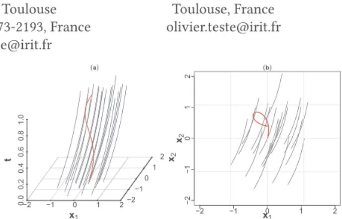
Figure 1: Example of 21 MFD (𝑝 = 2) with one shape persistent outlier in red. (a) (𝑡, 𝑥𝑖1, 𝑥𝑖2)representation. (b)

(𝑥𝑖1, 𝑥𝑖2)representation i.e. projection along 𝑡-axis.

Detecting atypical behaviors is referred as outlier or anomaly detection. An outlier is defined as a sample which is rare and very different from the rest of the data set based on some measure [1]. A taxonomy of functional outliers into two classes has been proposed by Hubert et al. [8]. First, an isolated outlier is defined as a sample which exhibits an extreme behavior for very few points 𝑡 . For instance a narrow vertical peak in the curve depicted by a parameter 𝑥𝑖𝑘w.r.t 𝑡 is named a magnitude isolated outlyingness

and a high horizontal translation in the curve is referred as shift isolated outlyingness. Second, a persistent outlier is a sample which never exhibits extreme behavior but deviates from inliers for many points 𝑡 , an example of shape persistent outliers is given in Fig.1. Persistent outliers can be divided into other sub-classes, see [8] for detailed examples. Note that an outlier can be of mixed type, i.e. a sample entailing several outlier classes. For an instance, one parameter has a shape persistent outlyingness and another one has an isolated outlyingness.

In this paper we focus on a geometric representation for out-lier detection in MFD and highlight the situation of outout-liers of mixed type. The MFD case is more challenging than the UFD one since the potential correlation between the 𝑝 parameters (i.e. how 𝑥𝑖𝑘 and 𝑥𝑖𝑘′are correlated w.r.t 𝑡 ) has to be taken into account

additionally to the individual variations of the single parameters w.r.t to 𝑡 [8]. Indeed contrary to outliers in UFD, where the outly-ingness of a sample only consists of an atypical variation w.r.t 𝑡 of a single parameter, in MFD the outlyingness of sample might be hidden in an atypical variation of the relationship between some parameters [8, 11] as well as an atypical variation of one of the 𝑝 parameters. Note that the representation of MFD we propose can also be used for other tasks than outlier detection (e.g. classification) as well as other geometric representations of 2D and 3D shapes which can be applied for the 𝑝 = 2 and 𝑝 = 3 (respectively) MFD cases [16].

1.2

Related work

The outlier detection in MFD is recent and has been addressed by statistical depth functions [18] originally proposed to provide

an outward-center ranking score, also named a depth score (e.g. in the interval [0, 1]), of multivariate data which are basically sample points in R𝑑. In this general multivariate data context, where each sample is regarded as a point in a 𝑑-dimensional point cloud, the first ranked samples are the most central ones within such point cloud and are seen as most representative, whereas the last ranked samples are the least central ones and thus they are likely to be outliers. Such ranking is ensured through the monotonicity property of the depth function (see [18] for the-oretical understanding of a depth function). Hence, the depth score can be viewed as an outlyingness score which reflects the degree of outlyingness at the sample level.

Some statistical depth functions have been extended first to handle UFD [3] and then MFD [2, 8]. The UFD extension consists in computing a depth function on 𝑥𝑖(𝑡), ∀𝑖 at each 𝑡 and then to

compute the integral over 𝑡 ∈ T of the resulting depth scores [3, 6] which in turn provides an average sample depth score for all 𝑖. Note that this extension is an aggregation of the depth function applied in a univariate manner since, for a given 𝑡 , {𝑥𝑖(𝑡)}𝑖 ≤𝑛is a

point cloud in R. Since {𝑋𝑖(𝑡)}𝑖 ≤𝑛forms a point cloud in R𝑝, the

MFD extension relies on the application of a depth function in a multivariate manner and integrates the depth scores as in the UFD case [2]. Such an extension suffers from important issues : (1) First, it is not sensitive enough to persistent outliers

be-cause their point-wise depth scores (i.e. for each 𝑡 ) do not differ from those of inliers. One can augment the MFD samples by adding some derivatives functions of the pa-rameters as supplementary (unobserved) papa-rameters but it increases both computations and the complexity of the data analysis.

(2) Second, even if the point-wise depth scores of an isolated outlier are different from those of an inlier, its sample depth score will be mixed with inliers because the integra-tion of the point-wise depth scores acts as an average. (3) Furthermore, since the capacity of the depth function to

capture different types of outlier is fundamental, outliers caused by abnormal correlation between the parameters (i.e. outliers of mixed type) are hard to detect. Such an abnormal correlation can result in outliers of mixed type. To address the first issue (1), and especially to detect shape persistent outliers, several depth functions have been proposed. Khunt and Rehage (𝐹𝑈 𝑁𝑇 𝐴) [9] proposed a depth function based on the intersection angles between a curve sample depicted by 𝑥𝑖𝑘 and {𝑥𝑗𝑘}𝑗 ≤𝑛,𝑗 ≠𝑖and then average these angles over both

their number and the parameters. Such method is not able to detect outliers caused by an abnormal correlation between the parameters and also isolated outliers because their depth function is only focused on shape persistent outliers.

To address the second issue (2) the integral can be replaced by the infimum as the aggregation of the point-wise depth scores, which avoids the masking of outliers having few different point-wise depth scores.

To address the third issue (3), Dai and Genton [4] proposed the directional outlyingness (𝐷𝑖𝑟 .𝑜𝑢𝑡 ), a point-wise depth function based on the direction of 𝑋𝑖(𝑡) in R𝑝toward the projection-depth

[17] of {𝑋𝑖(𝑡)}𝑖 ≤𝑛. To compute the sample depth score, the

point-wise depth scores are aggregated through an integral over T which is further decomposed into an average component and a variance-like component. Such sample depth score decomposi-tion enables to detect multiple outliers and also to identify their class by analyzing how the two depth components are distributed

according the other sample depth scores (e.g. samples with high variance-like component value are likely persistent shape out-liers and samples with high average component value are likely isolated outliers). However, to detect persistent shape outliers, the direction of 𝑋𝑖(𝑡) is not a sufficient feature and further

geo-metrical representation has to be considered.

1.3

Contribution

In this paper, we propose a different framework than the sta-tistical depth to remedy these issues by treating MFD as trajec-tories in R𝑝from which we extract geometrical features such as the curvature. Such geometrical features are computed by interpretable (from a geometric standpoint) aggregation func-tions, named mapping functions in the sequel, which combine some derived functions (e.g. derivatives, integral) from the MFD. We then apply a state-of-the-art algorithm on the geometrical MFD representation to achieve the outlier detection. Considering MFD in a geometric manner enables to implicitly capture the correlation between the 𝑝 parameters w.r.t 𝑡 and thus to detect different classes of outliers as well as mixed types. Moreover, such combination results in a more robust outlier detection method e.g. when there are more than 5% of outliers in the training set. Thus, we both take benefit from outlier detection algorithm for multivariate data as well as the geometry of the curve (i.e. the geometry of 𝑋𝑖 in R𝑝and the geometry of each parameter 𝑥𝑖𝑘

w.r.t 𝑡 ).

2

FUNCTIONAL DATA REPRESENTATION

The first step in functional data analysis is to approximate the unknown function, 𝑋𝑖:T → R𝑝, underlying the noisy

measure-ment samples 𝑋𝑖(𝑡1), ..., 𝑋𝑖(𝑡𝑚𝑖) where 𝑚𝑖is the number of

mea-surements for each parameter of the sample 𝑖, by an approxima-tion funcapproxima-tion ˜𝑋𝑖defined as 𝑋𝑖. Note that no assumption is made

on the distribution of the measurement points {𝑡1...𝑡𝑚𝑖} = 𝑡𝑖•,

thus the functional data representation can deal with sparse mea-surements as well as uniform ones.

The functional approximation step aims at removing the noise and thus enables to achieve accurate evaluations of some derived functions that we need for the mapping function computation. This section introduces how ˜𝑋𝑖 =( ˜𝑥𝑖1, ..., ˜𝑥𝑖𝑘, ..., ˜𝑥𝑖𝑝) is specified

as well as it is inferred from the data.

2.1

Functions as a basis expansion

First, we specify the functional form of the approximation func-tion as a finite linear combinafunc-tion of basis funcfunc-tions, where each basis function depends on 𝑡 ∈ T . Suppose we want to approxi-mate 𝑥𝑖𝑘. Intuitively, it aims to represent ˜𝑥𝑖𝑘with a small number

of "specific functions", each one being able to capture some local features of 𝑋𝑖 in hopes to recover it with a small approximation

error. Hence, the following form is given for ˜𝑥𝑖𝑘 [13],

∀𝑡 ∈ T , ˜𝑥𝑖𝑘(𝑡) = 𝐿𝑖𝑘

Õ

𝑙 =1

𝛼𝑖𝑘𝑙𝜙𝑙(𝑡) = 𝜶⊤𝑖𝑘𝝓 (𝑡 ) (1)

where 𝝓 (𝑡 ) = {𝜙𝑙(𝑡)}1≤𝑙 ≤𝐿𝑖𝑘 is a vector of orthonormal basis

functions at 𝑡 for some 𝐿𝑖𝑘 ∈ N∗(referred as the basis size) with

fewer basis functions than sampled observation points (𝐿𝑖𝑘 ≪

𝑚𝑖), and 𝜶_𝑖𝑘⊤ = _{{𝛼𝑖𝑘𝑙}}1≤𝑙 ≤𝐿𝑖𝑘 is the coefficient vector which

element 𝛼𝑖𝑘𝑙 is the importance of the 𝑙-th basis function. The

Here we consider that 𝑥𝑖𝑘are smooth and so we choose the

B-spline basis of functions which are basically piece-wise polyno-mial functions. If the data were periodic data, one could choose the Fourier basis. We refer to [13] for a discussion on the choice of basis functions. Note that from the functional approximation Eq.1, one can easily compute some derivatives or integral based functional data since by linearity,

𝐷𝑞_𝑥˜_𝑖𝑘= 𝐿𝑖𝑘 Õ 𝑙 =1 𝛼𝑖𝑘𝑙𝐷𝑞𝜙𝑙(𝑡) (2) where 𝐷𝑞= d𝑞

d𝑡𝑞 is the 𝑞−th derivative operator, provided that

the basis functions 𝜙𝑙are differentiable at the 𝑞-th order.

2.2

Inference

Assuming the data were sampled with a white noise 𝜖𝑖 𝑗, i.e.

𝑥𝑖𝑘(𝑡𝑖 𝑗) = ˜𝑥𝑖𝑘(𝑡𝑖 𝑗) + 𝜖𝑖 𝑗where 𝜖𝑖 𝑗is independent from ˜𝑥𝑖𝑘(𝑡𝑖 𝑗),

we can compute the coefficient vector 𝜶𝑖𝑘 by minimizing the

following penalized least-squares criteria: 𝑱𝜆𝑘(𝜶𝑖𝑘) = k𝑥𝑖𝑘(𝑡𝑖•) − Φ𝑖𝑘𝜶𝑖𝑘k

2

+ 𝜆𝑘𝜶𝑖𝑘⊤R𝑖𝑘𝜶𝑖𝑘 (3)

where k·k stands for the 𝑙2-norm, Φ_𝑖𝑘=_{{𝜙𝑙(𝑡𝑖 𝑗})}1≤ 𝑗 ≤𝑚𝑖,1≤𝑙 ≤𝐿𝑖𝑘

is the 𝑚𝑖× 𝐿𝑖𝑘matrix containing all the 𝐿𝑖𝑘basis functions

evalu-ated at the measurement points 𝑡𝑖• and

R_𝑖𝑘 ={∫_T𝐷𝑞𝝓𝑗(𝑡)𝐷𝑞𝝓𝑚(𝑡)d𝑡)}1≤ 𝑗,𝑚 ≤𝐿𝑖𝑘 is a 𝐿𝑖𝑘× 𝐿𝑖𝑘positive

semi-definite matrix containing the inner products of the 𝑞-th derivative of the basis functions which enforces the approxima-tion funcapproxima-tion to have a small 𝑞-th derivative i.e. to vary smoothly; 𝜆𝑘> 0 is a hyper-parameter controlling the weight of the penalty and can be set to 0 for no penalization. In practice it is common to choose 𝑞 = 1 or 𝑞 = 2 (i.e to penalize the velocity or the acceleration) and to compute 𝜆𝑘by cross-validation.

Equaling the gradient of 𝑱𝜆𝑘to 0 w.r.t 𝜶𝑖𝑘leads to the

mini-mizer in Eq.4 [13] which is a special case of the ridge regression solution:

𝜶∗_{𝑖𝑘,𝜆}=(Φ_𝑖𝑘⊤Φ_{𝑖𝑘+ 𝜆𝑘}R_𝑖𝑘)−1Φ⊤

𝑖𝑘𝑥𝑖𝑘(𝑡𝑖•) (4)

The estimated coefficient vector 𝜶_{𝑖𝑘,𝜆}∗ can then be plugged in Eq.1 to evaluate ˜𝑥𝑖𝑘over an arbitrary discretization of T .

3

MAPPING FUNCTION

We propose to regard MFD as paths in R𝑝to highlight some un-derlying shape outlyingness features corresponding to a change in the relationship between the parameters. We feature this change with a mapping function that we define as a geometric aggregation of the 𝑝 parameters. We refer to [15] for an intro-duction to shape analysis from functional data.

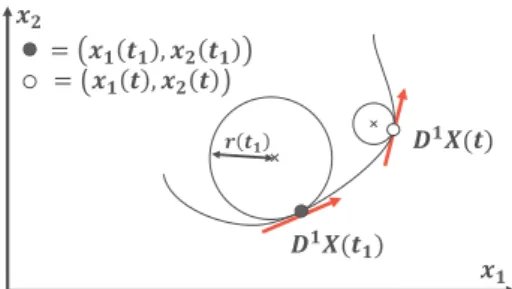
In this section, we present the curvature as an example of mapping function. The curvature is a measure of how much bended a curve is, more formally how the curve locally deviates from the tangent line, see Fig.2. It is defined as:

𝜅 (𝑡 ) = k𝐷1( 𝐷 1 𝑋 (𝑡 ) k𝐷1_{𝑋 (𝑡 ) k}) k k𝐷1_{𝑋 (𝑡 ) k} (5)

where k·k denotes the Euclidean norm in R𝑝. One can interpret 𝜅 in Eq.(5) as follows: 𝐷

1

𝑋 (𝑡 )

k𝐷1_{𝑋 (𝑡 ) k} gives the direction vector (i.e

the normalized tangent vector), therefore 𝐷1 𝐷

1

𝑋 (𝑡 )

k𝐷1_{𝑋 (𝑡 ) k}gives the

change direction vector and the denominator k𝐷1𝑋 (𝑡 ) k aims to relate the change of direction w.r.t the tangent vector, i.e. how the direction vector varies w.r.t a tangent line. Consequently, the

!_"(# !) !_"(#) $% $! = $! # , $%# = $!#!, $% #! & #!

Figure 2: Curvature mapping 𝜅. The curvature measures how large the radius of the tangent circle is. Here, in the neighbourhood of the curve at 𝑡1(dark-grey dot), the

tan-gent vector 𝐷1𝑋 (𝑡1) keeps the same direction, hence the

tangent circle has a large radius (𝑟 (𝑡1) = 1

𝜅 (𝑡1)) resulting in

a small curvature. In the neighbourhood of the curve at 𝑡 (white dot), the tangent vector 𝐷1𝑋 (𝑡 ) quickly changes di-rection, hence the tangent circle has a lower radius i.e. a higher curvature than at 𝑡1.

curvature mapping can highlight functional outliers which curve exhibits a different bended shape than the other samples.

Thus if a curve abnormally changes direction (i.e. it deviates from a tangent line) w.r.t most of the data set, then the curvature mapping can highlight outliers. As a result, if the curve 𝑋𝑖depicts

a line (i.e. the parameters are linearly correlated w.r.t 𝑡 ), then the curvature is constant w.r.t 𝑡 since the directions do not vary in R𝑝_{. Clearly, this is a geometric characterization of MFD.}

From the reconstructed samples { ˜𝑋𝑖}𝑖 ≤𝑛, transformed to UFD

by the mapping function, we detect the outliers with state-of-the-art algorithms initially proposed to deal with multivariate data (not functional). Here we use Isolation-Forest (𝑖𝐹𝑜𝑟 ) [10] and One-class SVM (𝑂𝐶𝑆𝑉 𝑀) [14] which are both unsupervised.

4

NUMERICAL EXPERIMENTS

We conducted an experimental study on real data. We com-pare our approach with state-of-the-art depth-based methods, 𝐹𝑈 𝑁𝑇 𝐴 and 𝐷𝑖𝑟 .𝑜𝑢𝑡 [4, 9] (Sec.1.2) which take the MFD as input.

4.1

Experimental procedure

We experiment our method on a well-known real data set of electrocardiogram (ECG) time series [7] also used in outlier de-tection in [4]. Such data set correspond to time series of electrical activity and can reveal abnormal heartbeat. The time series are UFD (with number of measurements 𝑚𝑖 = 85_{, ∀𝑖) and in order} to show the applicability of our approach in the MFD case, we augment the original UFD data to MFD (𝑝 = 2, bivariate) by adding the square of the initial time series. We did not add some derivatives-based functions as supplementary parameters since it is already considered by our mapping function (see Eq.5).

We evaluate our approach through multiple random splittings. We randomly split the data into a training and a test set. We generate the training set by setting the ratio of outliers (referred as the contamination level 𝑐) to 5, 10, 15, 20 and 25%. For each value of 𝑐, we repeat the random splitting 50 times, we fit 𝑖𝐹𝑜𝑟 and 𝑂𝐶𝑆𝑉 𝑀 on the training set and compute the average and standard deviation Area Under (AUC) the Receive Operating Curve (ROC) on the corresponding test set. We present the results in Fig.3 and discuss them in Sec.4.3.

For each sample and each variable 𝑥𝑖𝑘∀𝑖, 𝑘 we use a B-spline

ba-sis of functions (piece-wise polynomial functions, [13]) to achieve the functional approximations and we select the basis sizes 𝐿𝑖𝑘

0.05 0.10 0.15 0.20 0.25 0. 75 0. 85 0. 95

AUC vs. contamination level

c AUC Dir.out FUNTA iFor(Curvmap) OCSVM(Curvmap)

Figure 3: AUC (vertical axis) and standard deviation (verti-cal segments’ length equals one standard deviation) from ECG data set - average results over 50 repetitions consid-ering five contamination levels 𝑐 (horizontal axis). trough a leave-one-out cross validation procedure. We evaluate each ˜𝑋𝑖 on the same regular grid of T with length 𝑚𝑖 = 85_{. We} compute the mapping function by combining the first and second derivatives, according to Eq.2 and Eq.5, and we apply 𝑖𝐹𝑜𝑟 and 𝑂𝐶𝑆𝑉 𝑀 on the resulting UFD.

4.2

Outlier detection step

We use 𝑖𝐹𝑜𝑟 and 𝑂𝐶𝑆𝑉 𝑀 as outlier detection algorithms on the UFD that our mapping function 𝜅 returns (Eq.5). 𝑖𝐹𝑜𝑟 and 𝑂𝐶𝑆𝑉 𝑀 are unsupervised and, like the depth-based methods, output a normalized outlyingness score for each sample. In prac-tice, in outlier detection one has not necessarily access to labeled samples, i.e. information depicting whether a sample is an outlier or not, but if he has, the labels can be combined with their corre-sponding outlyingness scores to learn an outlyingness threshold that can best discriminate outliers from inliers. Such a threshold can be learned from the ROC as well as an imbalanced classifi-cation algorithm [5, 12] in a one dimensional manner from the scores. Here, we do not learn any threshold and only consider the label information for empirical demonstration purpose, i.e. by computing the AUC on the test set.

4.3

Discussion of the results

From the results in Fig.3, we see that we outperform the two depth-based methods for all the contamination levels in aver-age and perform equally in terms of standard deviation. Since 𝐹𝑈 𝑁𝑇 𝐴 is only able to detect persistent shape outliers and 𝐷𝑖𝑟 .𝑜𝑢𝑡 is expected to detect isolated as well as persistent outliers1, we can deduce that the abnormal class (i.e.outliers) in the ECG data set not only contains persistent shape outliers but also isolated ones or outliers of mixed type which are well discriminated by the curvature mapping function. Thus the curvature mapping enables to detect mixed type outliers.

Moreover, we note that as 𝑐 increases both 𝑖𝐹𝑜𝑟 (𝐶𝑢𝑟𝑣𝑚𝑎𝑝)

and 𝑂𝐶𝑆𝑉 𝑀 (𝐶𝑢𝑟𝑣𝑚𝑎𝑝) still outperform the baselines. Hence, we

show that our combination of outlier detection algorithm with MFD mapped to a geometrical representation is more robust to the presence of outliers in the training set than the baselines. We note that OCSVM degrades as 𝑐 increases. It is due to the 𝜈 hyper-parameter (we tune it on the training set with a 5-fold cross validation) corresponding to an estimate of contamination level in

1_{Justification can be found in the experiments in [4] which were conducted on}

several synthetic data sets where each one contains a unique type of outlier.

the training set. We observed that such hyper-parameter is hard to tune as 𝑐 increases and thus could decrease the performance w.r.t 𝑐.

5

CONCLUSION AND FUTURE WORK

We propose an approach to detect outliers in MFD. It consists in computing a geometrical representation of MFD followed by an outlier detection algorithm. We compare our approach with recent depth-based methods which handle MFD as input.

Through one example of mapping function, we show that the geometrical representation of MFD is well suited to detect outliers of mixed type. However, it is hard to interpret what such mixed type outliers are made up: given a detected outlier, ideally one would like to access to the amount of the different outlyingness classes e.g. the amount of shape persistence and shift isolated outlyingness. As future work, a mean to achieve such an interpretability is first to detect some specific outliers with depth functions, second to train outlier detection algorithms (combined with a mapping function) on training sets containing each one a unique class of outlier previously detected and then to average all the models trained to form an ensemble one. As a result, one could know which model(s) in the ensemble most contribute to the outlyingness and deduce the outlyingness composition.

ACKNOWLEDGMENTS

This work is supported by ANRT within the CIFRE framework (grant N°2017-1391).

REFERENCES

[1] Charu C Aggarwal and Philip S Yu. 2001. Outlier detection for high dimen-sional data. In ACM Sigmod Record, Vol. 30. ACM, 37–46.

[2] Gerda Claeskens, M Hubert, Leen Slaets, and K Vakili. 2014. Multivariate Functional Halfspace Depth. J. Amer. Statist. Assoc. 109, 505 (2014), 411–423. [3] Antonio Cuevas and Manuel Febrero. 2007. Robust estimation and

classifica-tion for funcclassifica-tional data via projecclassifica-tion-based depth noclassifica-tions. Computaclassifica-tional Statistics 22, 3 (2007), 481–496.

[4] Wenlin Dai and Marc G. Genton. 2019. Directional outlyingness for multivari-ate functional data. Computational Statistics and Data Analysis 131 (2019). [5] Shounak Datta and Swagatam Das. 2015. Near-Bayesian support vector

ma-chines for imbalanced data classification with equal or unequal misclassifica-tion costs. Neural Networks 70 (2015), 39–52.

[6] Ricardo Fraiman and Graciela Muniz. 2001. Trimmed means for functional data. Test 10, 2 (2001), 419–440.

[7] Ary L Goldberger, Luis AN Amaral, Leon Glass, Jeffrey M Hausdorff, Pla-men Ch Ivanov, Roger G Mark, Joseph E Mietus, George B Moody, Chung-Kang Peng, and H Eugene Stanley. 2000. PhysioBank, PhysioToolkit, and PhysioNet: components of a new research resource for complex physiologic signals. Circulation 101, 23 (2000), e215–e220.

[8] Mia Hubert, Peter J. Rousseeuw, and Pieter Segaert. 2015. Multivariate func-tional outlier detection. Statistical Methods and Applications 24, 2 (2015). [9] Sonja Kuhnt and André Rehage. 2016. An angle-based multivariate functional

pseudo-depth for shape outlier detection. Journal of Multivariate Analysis. 146 (2016), 325–340.

[10] Fei Tony Liu, Kai Ming Ting, and Zhi-Hua Zhou. 2008. Isolation Forest. In ICDM.

[11] Sara López-pintado, Yin Sun, Juan K Lin, and Marc G. Genton. 2014. Simplicial band depth for multivariate functional data. Advances in Data Analysis and Classification 8, 3 (2014), 321–338.

[12] Art B Owen. 2007. Infinitely imbalanced logistic regression. Journal of Machine Learning Research. 8 (2007), 761–773.

[13] James O. Ramsay and B.W. Silverman. 2006. Functional Data Analysis. Springer. [14] Bernhard Schölkopf, John C Platt, John Shawe-Taylor, Alex J Smola, and Robert C Williamson. 2001. Estimating the support of a high-dimensional distribution. Neural computation 13, 7 (2001), 1443–1471.

[15] Anuj Srivastava and Eric P Klassen. 2016. Functional and Shape Data Analysis. Springer.

[16] Weiyi Xie, Oksana Chkrebtii, and Sebastian Kurtek. 2019. Visualization and Outlier Detection for Multivariate Elastic Curve Data. IEEE Transactions on Visualization and Computer Graphics (2019).

[17] Yijun Zuo et al. 2003. Projection-based depth functions and associated medians. The Annals of Statistics 31, 5 (2003), 1460–1490.

[18] Yijun Zuo and Robert Serfling. 2000. General Notions of Statistical Depth Function. The Annals of Statistics. 28, 2 (2000), 461–482.