Tomographic Slug and Pumping Tests Comparison 1/22 Submitted to Environmental Earth Sciences: NovCare 2015 Thematic Issue
1 2
Comparison of slug and pumping tests for hydraulic tomography
3
experiments: A practical perspective
4 5
Daniel Paradis1, René Lefebvre2, Erwan Gloaguen2, and Bernard Giroux2 6
7
1: Geological Survey of Canada, 490 rue de la Couronne, Quebec City, Canada G1K 9A9 8
2: Institut national de la recherche scientifique, Centre Eau Terre Environnement (INRS-ETE), 9
490 rue de la Couronne, Quebec City, Canada G1K 9A9 10
11
Corresponding author: Daniel Paradis 12
Phone: (418) 654-3713 Fax: (418) 654-2604 E-mail: [email protected] 13
14 15
KEYWORDS: Aquifer characterization, Heterogeneity, Hydraulic tomography, Slug tests, 16
Pumping tests, Resolution analysis, Principle of reciprocity 17 18 1 2 3 4 5 6 7 8 9 10 11 12 13 14 15 16 17 18 19 20 21 22 23 24 25 26 27 28 29 30 31 32 33 34 35 36 37 38 39 40 41 42 43 44 45 46 47 48 49 50 51 52 53 54 55 56 57 58 59 60 61
ABSTRACT 19
20
Hydraulic tomography is the simultaneous analysis of several hydraulic tests performed in 21
multiple isolated intervals in adjacent wells to image heterogeneous hydraulic property fields. In 22
this study, we compare the resolutions associated with hydraulic tomography experiments carried 23
out with slug tests and pumping tests for simple configurations with hydraulic property values 24
representative of an extensively studied littoral aquifer. Associated test designs (e.g., pumping 25
rates, test durations) and the validity of the principle of reciprocity are also assessed. For this 26
purpose, synthetic tomography experiments and their associated sensitivity matrices are 27
generated using a radial flow model accounting for wellbore storage. The resolution analysis is 28
based on a pseudo-inverse analysis of the sensitivity matrix with a noise level representative of 29
field measurements. Synthetic experiments used equivalent perturbations for slug tests and 30
pumping tests. Even though pumping tests induce a drawdown in observation intervals that is 31
three times larger than head changes due to slug tests, resolutions for hydraulic conductivities 32
(horizontal and vertical) are similar for the two tests and slightly lower for specific storage with 33
pumping. However, experiments with pumping require fifty times more water and are seven 34
times longer to perform than experiments with slug tests. Furthermore, reducing pumping rates 35
to limit disposal of water or test durations to decrease field data acquisition time would 36
considerably lower resolutions for either scenario. Analyses are done using all available stressed 37
and observation intervals as required by the non-applicability of the principle of reciprocity for 38
slug tests and pumping tests with important wellbore storage. This study demonstrates concepts 39
that have important implications for the performance and analysis of hydraulic tomography 40 experiments. 41 42 4 5 6 7 8 9 10 11 12 13 14 15 16 17 18 19 20 21 22 23 24 25 26 27 28 29 30 31 32 33 34 35 36 37 38 39 40 41 42 43 44 45 46 47 48 49 50 51 52 53 54 55 56 57 58 59 60
1 Introduction
43
Knowledge of the hydraulic heterogeneity that controls flow and transport in aquifer systems, 44
such as preferential flow paths and impermeable barriers, is essential for sound groundwater 45
resource protection. Slug tests and pumping tests are common field experiments used to estimate 46
the hydraulic properties of aquifer systems (Kruseman and de Ridder, 2000). A slug test consists 47
of inducing an instantaneous change in water level in a well, whereas a pumping test involves 48
withdrawing water out of a well at a controlled, generally constant, rate. For both kinds of 49
hydraulic tests, water level response is measured in one or more surrounding observation wells 50
and in the stressed well itself. The area affected by a hydraulic test is a function of the hydraulic 51
diffusivity defined by the ratio of hydraulic conductivity (K) and specific storage (Ss). The larger
52
the hydraulic diffusivity, the larger will be the response in the observation well and the farther 53
from the stressed well will it be possible to measure the response with a good signal to noise 54
ratio . Several authors have proposed the use of hydraulic tomography to define heterogeneous 55
hydraulic property fields (e.g., Tosaka et al., 1993; Gottlieb and Dietrich, 1995; Butler et al., 56
1999; Yeh and Liu, 2000; Bohling et al., 2002; 2007; Brauchler et al., 2003, 2010, 2011, 2013; 57
Zhu and Yeh, 2005; Illman et al., 2007, 2008; Fienen et al., 2008; Cardiff et al., 2009; Illman et 58
al., 2009; Berg and Illman, 2011, 2013, 2015; Cardiff and Barrash, 2011; Huang et al., 2011; 59
Cardiff et al., 2012; Sun et al., 2013; Paradis et al., 2015; 2016). Hydraulic tomography is the 60
simultaneous analysis of several hydraulic tests performed in multiple wells or multiple isolated 61
intervals in wells, which provides a better resolution capability of hydraulic property fields than 62
conventional hydraulic tests (Butler, 2005). Analysis of hydraulic tomography data is essentially 63
related to inverse problems with issues related to non-uniqueness of the solution as the number 64
of unknown parameters is usually greater than the number of measurements (under-determined 65
problem) or the data do not contain enough information about the model parameters (rank-66
deficient problem) due to the physics of the problem and experimental configuration (e.g., 67
Carrera and Neuman, 1986; Yeh and Liu, 2000; Tonkin and Doherty, 2005; Illman et al., 2008; 68
Bohling, 2009; Xiang et al., 2009; Bohling and Butler, 2010; Huang et al., 2011; Liu and 69
Kitanidis, 2011; Paradis et al., 2015, 2016). While regularization for constraining the number of 70
possible solutions is an important topic (e.g., Tikhonov, 1963; Tikhonov and Arsenin, 1977; 71
Kitanidis, 1995; Vasco et al., 1997; Carrera and Neuman, 1986; Yeh and Liu, 2000; Doherty, 72 4 5 6 7 8 9 10 11 12 13 14 15 16 17 18 19 20 21 22 23 24 25 26 27 28 29 30 31 32 33 34 35 36 37 38 39 40 41 42 43 44 45 46 47 48 49 50 51 52 53 54 55 56 57 58 59 60 61
2003; Caers, 2005; Rubin and Hubbard, 2005; Tonkin and Doherty, 2005; Carrera et al., 2005; 73
Fienen et al., 2008; Illman et al., 2008; Berg and Illman, 2011; Cardiff and Barrash, 2011; 74
Huang et al., 2011; Cardiff et al., 2012; Sun et al., 2013; Soueid Ahmed et al., 2014; Zha et al., 75
2014), this paper focuses rather on some practical aspects related to hydraulic tomography, 76
which is of crucial importance to guide practitioners involved in hydraulic property 77
characterization either in terms of estimates accuracy or field efficiency. 78
79
The ability of a hydraulic experiment to resolve hydraulic property fields from observations can 80
be understood through the analysis of the sensitivity of head or drawdown to the parameters 81
associated with the aquifer system to characterize (Menke, 1989; Aster, 2005). Sensitivity 82
magnitudes and correlations indicate which parameters can be better resolved. For example, it 83
has been recognized by Butler and McElwee (1990) that varying the magnitude and frequency of 84
the pumping rate scheme of a pumping test can increase parameter resolutions by increasing 85
sensitivity magnitudes while simultaneously constraining sensitivity correlations. While constant 86
rate pumping tests are the most used tests for hydraulic tomography (see the comprehensive 87
summary of previously published studies dedicated to hydraulic tomography provided by Cardiff 88
and Barrash, 2011), few efforts have been dedicated to understanding the impact of test initiation 89
methods on the resolution of hydraulic property fields. Actually, since slug and pumping tests 90
generate very different hydraulic perturbations, it would be worth assessing whether those tests 91
produce different parameter resolution characteristics for hydraulic tomography experiments. 92
Indeed, early times hydraulic response for a pumping test is known to be mostly sensitive to 93
parameters between the stressed and observation wells, whereas the relative influence of 94
parameters outside the inter-well region increases as the drawdown spreads away from the 95
observation well (Oliver, 1993; Leven et al., 2006). On the other hand, it is generally considered 96
that only the immediate vicinity of the stressed well can be resolved with a slug test because the 97
change in hydraulic head pulse is sharply vanishing away from the stressed well (Ferris and 98
Knowles, 1963; Rovey and Cherkauer, 1995). 99
100
The main objective of this study is then to compare the resolutions associated with tomography 101
experiments carried out with slug tests and pumping tests. In particular, we are interested by the 102
resolution of horizontal hydraulic conductivity (Kh), K anisotropy (ratio of vertical and horizontal
103 4 5 6 7 8 9 10 11 12 13 14 15 16 17 18 19 20 21 22 23 24 25 26 27 28 29 30 31 32 33 34 35 36 37 38 39 40 41 42 43 44 45 46 47 48 49 50 51 52 53 54 55 56 57 58 59 60
K, Kv/Kh), and Ss. Moreover, choices in hydraulic test design (e.g., test stress: pumping rate and
104
initial head, test duration) are often made to get around some technical difficulties often 105
encountered during field tomography experiments, such as desaturation of the stressed interval, 106
noisy measurements and excessive test durations. Thus, in an effort to maximize the quality of 107
the information contained in field data, often-acquired at large expenses, we also assess the 108
impact of some field practices associated to the realization of hydraulic tests and verify the 109
validity of the principle of reciprocity for both kinds of tests. 110
111
After presenting the general approach followed to evaluate the resolution matrix of a tomography 112
experiment in Section 2, we verify the applicability of the principle of reciprocity for slug and 113
pumping tests and we discuss the implications for acquisition and analysis of tomography data in 114
Section 3. Then, Section 4 presents a comparison of resolution for tomography experiments 115
using slug tests and pumping tests as well as the impact of reduced test stresses (pumping rates 116
and initial heads) and test durations. Finally, we summarize and discuss the main findings of this 117
study in Section 5. 118
2 General approach for the evaluation of the resolution matrix
119
The observations (head or drawdown) made during a hydraulic test are sensitive to the hydraulic 120
properties or parameters of the aquifer system at locations reached by the perturbation induced 121
by the test (Vasco et al., 1997). Parameter sensitivity is the ratio of the change in the 122
observations to a unit relative change in a parameter value. The relative magnitude of the 123
sensitivity for different parameters indicates which parameters can be better resolved from the 124
observations. Also, parameters that have dissimilar (non-correlated) temporal sensitivity patterns 125
throughout a test can be resolved separately because they have different effects on observations. 126
A resolution matrix combines sensitivities from a number of observations and for a number of 127
parameters into a single measure related to each parameter, which integrates the effects of 128
sensitivity magnitudes and correlations, and that can be analyzed to assess the ability to resolve 129
parameters from tomography experiments. Figure 1 illustrates the general approach followed to 130
evaluate the resolution matrix of a tomography experiment carried out with slug tests or pumping 131
tests. Further details about this approach proposed by Clemo et al. (2003) that is summarized 132
below can be found in Bohling (2009) and Paradis et al. (2015). 133 4 5 6 7 8 9 10 11 12 13 14 15 16 17 18 19 20 21 22 23 24 25 26 27 28 29 30 31 32 33 34 35 36 37 38 39 40 41 42 43 44 45 46 47 48 49 50 51 52 53 54 55 56 57 58 59 60 61
134
1. Forward modeling and sensitivity calculation. To simulate hydraulic tests (slug and 135
pumping tests) and to compute sensitivities of the synthetic tomography experiments, we used 136
the numerical simulator lr2dinv (Bohling and Butler, 2001). This simulator is a two-dimensional 137
(2D) axisymmetric finite-difference model that describes flow to a partially penetrating well in 138
response to an instantaneous change in water level (e.g., slug test) or to a pumping stress in a 139
confined aquifer through the radial groundwater flow equation. The simulator also allows the 140
explicit simulation of wellbore storage effects and placement of packer intervals in the stressed 141
well. 142
143
Using lr2dinv, the sensitivity matrix elements are constructed by a sequence of groundwater flow 144
simulations, one simulation per parameter grid cell, in which each hydraulic property in a single 145
cell is slightly perturbed (1%) from its original value and the differences in head or drawdown 146
are noted. Each Jm,n element in the sensitivity matrix represents the normalized sensitivity of the
147
head or drawdown at a given time and location, hm, to one of the model parameter, pn:
148 149
J = Jm,n = pn∂hm
∂pn (1)
150
The head or drawdown index m runs over all observation times and locations for all simulated 151
tests, and pn represents either the Kh, Kv/Kh or Ss value associated with each cell in the parameter
152
grid. It should be noted that groundwater flow associated with each tomography experiment is 153
nonlinear, and we thus assume that the sensitivity matrix with its elements given by (1) provides 154
a close approximation of the behavior of the nonlinear flow in the vicinity of the model 155
parameters used for each synthetic simulations given the fact that small perturbations are used to 156
compute sensitivities (Bohling, 2009). Details about mathematical formulation and numerical 157
implementation can be found in Bohling and Butler (2001) and Butler and McElwee (1995). 158
159
For all synthetic simulations, we use a 2D simulation grid with 43 cells of logarithmically 160
increasing dimension along the radial axis encompassing the stressed and observation wells and 161
26 cells of dimension equal to 0.3048 m (1 foot) along the vertical axis. This discretization 162 4 5 6 7 8 9 10 11 12 13 14 15 16 17 18 19 20 21 22 23 24 25 26 27 28 29 30 31 32 33 34 35 36 37 38 39 40 41 42 43 44 45 46 47 48 49 50 51 52 53 54 55 56 57 58 59 60
places the zero-head outer boundary of the model very far from the stressed well (about 111 m), 163
so that it has negligible effects on simulated heads or drawdown at the stressed and observation 164
wells. Confined conditions are also assumed to define lower and upper boundary conditions. 165
Slug tests are simulated by modifying the initial head condition at the cells representing the 166
stressed interval, with all other heads in the model set to zero, in order to produce an 167
instantaneous head perturbation into the aquifer. And, pumping tests are simulated through the 168
boundary condition by specifying the pumping rate in the stressed interval. Note that to avoid 169
desaturation of the stressed interval (water level below the top of the screen) slug tests and 170
pumping tests are simulated by injecting water into the synthetic aquifer. Specific parameter grid 171
discretization and parameter values for each synthetic experiment discussed in this study are 172
presented later in their respective section. 173
174
2. Moore-Penrose pseudo-inverse and resolution matrix.Given a vector m of n parameters to 175
be estimated, the Moore-Penrose pseudo-inverse Jp† (Moore, 1920; Penrose, 1955) can be used in 176
computing a least-squares and minimum length solution m† from a data vector d of m 177
observations (head or drawdown) as (Menke, 1989; Aster, 2005): 178
179
m† = Jp†d (2)
180
where Jp† is the sensitivity matrix J retaining the p largest singular values and vectors of its
181
singular value decomposition corresponding to the most strongly resolved parameters. Note that 182
the Moore-Penrose pseudo-inverse is a convenient way of analyzing the information content of 183
least-squares inverse problems (e.g., Bohling, 2009; Paradis et al, 2015) without having to 184
optimize an objective function that could be computationally intensive. If the true model of 185
parameters are represented by the vector m and the corresponding true data vector is represented 186
by d=Jm, then the estimated parameter vector from the pseudo-inverse m† can be expressed 187
from (2) as (Menke, 1989; Aster, 2005): 188 189 m† = Jp†Jm = Rm (3) 190 4 5 6 7 8 9 10 11 12 13 14 15 16 17 18 19 20 21 22 23 24 25 26 27 28 29 30 31 32 33 34 35 36 37 38 39 40 41 42 43 44 45 46 47 48 49 50 51 52 53 54 55 56 57 58 59 60 61
The matrix multiplying the true model of parameters m is called the resolution matrix: 191
192
R= Jp†J (4)
193
where the elements of R are indicators of the relative magnitude and correlation between 194
parameter sensitivities resulting from the pseudo-inverse. For this study, only the diagonal 195
elements of R that indicate the resolution of each parameter are analyzed. The values of diagonal 196
elements are between 0 and 1: a value of 0 means that a parameter cannot be resolved from the 197
observations, whereas a value of 1 means it can be perfectly resolved. Discussion about the 198
information contained in the entire resolution matrix can be found in Menke (1989) and Aster 199
(2005). 200
201
To get a common basis of comparison among the different tomography experiments using slug 202
tests and pumping tests, we select for each experiment the number of p singular values and 203
vectors in (4) according to a predefined level of error in parameter estimates resulting from the 204
pseudo-inverse. As proposed by Clemo et al. (2003), p can indeed be selected by considering d 205
in (2) as the random noise in the observations η and m as the error in the parameter estimates 206
Δm†, which leads to the following: 207
208
Δm† = Jp†η (5)
209
Thus, for a given level of parameter error, defined here as the root-mean-square of the norm of 210
Δm†, the number of p singular values and vectors to retain for the evaluation of the resolution 211
matrix in (4) is selected using (5) (see Bohling, 2009). For this study, we choose an error Δm† of 212
0.1 (average relative error of 10%) and define a Gaussian noise η (mean of zero; standard 213
deviation of 2x10⁻⁴ m) realistic of field experimentations (e.g., Bohling, 2009; Paradis et al., 214 2015). 215 216 Figure 1 217
3 Verification of the principle of reciprocity
218 4 5 6 7 8 9 10 11 12 13 14 15 16 17 18 19 20 21 22 23 24 25 26 27 28 29 30 31 32 33 34 35 36 37 38 39 40 41 42 43 44 45 46 47 48 49 50 51 52 53 54 55 56 57 58 59 60
In this section, we investigate the applicability of the principle of reciprocity for slug tests and 219
pumping tests as it may have implications for the acquisition and analysis of tomographic data, 220
and consequently on parameter resolutions as well. The principle of reciprocity states that, as 221
long as wellbore storage effects can be neglected, reciprocal tests for which the role of the 222
stressed and observation intervals are interchanged produce identical observation interval 223
responses regardless of the degree of heterogeneity (see proof in McKinley et al., 1968). To 224
verify this principle, we simulate head and drawdown for reciprocal tests that are symmetrical 225
(Figure 2a) and asymmetrical (Figure 3a) with respect to the heterogeneity in Kh, Kv and Ss. Thus
226
for both models, reciprocal tests are simulated by varying each hydraulic property of layer 2 one 227
at a time (black layers in Figures 2a and 3a) while holding all other properties unchanged (Table 228
1). We note also that stressed and observation interval locations in Figures 2a and 3a are 229
symmetrical to the upper and lower no-flow boundaries to avoid misinterpretation of the 230
reciprocal tests. Wellbore storage is also only simulated in the stressed intervals as we assume 231
that wellbore storage effects in straddled observation intervals with packers can be neglected 232
(Sageev, 1986; Novakowski, 1989). 233
234
Figures 2b and 2c present results of the reciprocal slug tests and pumping tests, respectively, for 235
the symmetrical cases. Obviously, reciprocal responses are indistinguishable whether the test is 236
initiated in well 1 or well 2 since those tests are performed under identical conditions (note that 237
reciprocal curves are superposed in Figure 2). Figures 3b and 3c show however that for the 238
asymmetrical cases, that the reciprocal head and drawdown responses in the observation 239
intervals are different when Kh and Kv are varied, which refutes the principle of reciprocity.
240 241
As suggested by the comparison of Figures 3c and 3d for reciprocal pumping tests considering 242
and neglecting wellbore storage, respectively, the refutation of the principle of reciprocity for 243
observation interval responses could be explained by a wellbore storage effect. Note that stressed 244
interval responses differ regardless of the degree of heterogeneity. In fact, for a pumping test in a 245
well with a large diameter, the total pumping rate (Q) set by the pump is the combined 246
contributions of flow rates coming from the wellbore (Qw) and the aquifer system (Qa)
247
(Dougherty and Babu, 1984). Wellbore storage supplies most of the initial pumped water, which 248
initially equals to Q and gradually decreases to zero when pumping continues. In contrast, the 249 4 5 6 7 8 9 10 11 12 13 14 15 16 17 18 19 20 21 22 23 24 25 26 27 28 29 30 31 32 33 34 35 36 37 38 39 40 41 42 43 44 45 46 47 48 49 50 51 52 53 54 55 56 57 58 59 60 61
contribution from the aquifer system is initially zero and gradually approaches Q when 250
drawdown is reaching steady-state. Also, the relative contributions of Qw and Qa that must
251
balance with Q vary according to the hydraulic properties surrounding the stressed well 252
(Q=Qa+Qw). Note here that we only consider wellbore storage due to water level change and not
253
from water compressibility. Thus, as the drawdown in an observation interval is controlled by the 254
flow at this location Qobs, which depends on Qa at the stressed interval and the heterogeneity
255
travelled by the hydraulic perturbation, reciprocal drawdown responses in Figure 3c differ 256
because Qa is different for each reciprocal test while the heterogeneity seen in reverse order by
257
the hydraulic perturbations is the same in the two directions of testing. For pumping tests where 258
wellbore storage can be neglected (Qw=0), Qa is independent of the heterogeneity surrounding
259
the stressed well and is equal to the same constant value of Q for the two reciprocal tests (Qa=Q),
260
which explains the identical reciprocal observation interval responses in Figure 3d. We note in 261
Figure 3c that reciprocal observation interval responses are identical at steady-state when 262
wellbore storage effect becomes negligible. Finally, a similar reasoning can be applied for slug 263
tests in Figure 3a where Qa is proportional to the decline of the water level in the the stressed
264
interval (Qa=Qw; Q=0), which is also controlled by the hydraulic properties surrounding the
265
stressed interval. 266
267
In summary, the principle of reciprocity as applied to observation interval responses is valid for 268
cases where wellbore storage effects can be neglected. This is not the case for slug tests or 269
pumping tests with large diameter boreholes. As a consequence, stressed and observation interval 270
responses must be recorded during field testing and used together in the analysis of hydraulic 271 tomography experiments. 272 273 Table 1 274 275 Figure 2 276 277 Figure 3 278
4 Comparison of resolutions for different hydraulic test designs
279 4 5 6 7 8 9 10 11 12 13 14 15 16 17 18 19 20 21 22 23 24 25 26 27 28 29 30 31 32 33 34 35 36 37 38 39 40 41 42 43 44 45 46 47 48 49 50 51 52 53 54 55 56 57 58 59 60
This section explores the effects of different hydraulic test designs used for tomography 280
experiments on parameter resolutions. In particular, we assess the effects of test initiation 281
methods (slug and pumping tests), reduced test stresses (initial heads and pumping rates) and 282
reduced test durations. 283
4.1 Effect of test initiation methods
284In this section, we compare the resolutions of two tomography experiments that use slug tests 285
and pumping tests, respectively. To compare parameter resolutions on a common basis over the 286
domain, we use a parameter grid with similar cell sizes. The simulation grid was thus divided 287
into 143 cells of 0.61 m in height, that corresponds to the length of the stressed interval, and, due 288
the logarithmic change in cell dimensions in the radial direction, the cells of the simulation grid 289
were merged laterally to obtain cell widths of approximately equal size (Figures 4a and 4b). 290
Sensitivities for the resolution analysis are also computed from a homogeneous and anisotropic 291
model with bulk average Kh, Kv/Kh and Ss values of 1×10⁻⁵ ms-1, 0.1 and 1×10⁻⁵ m-1, respectively.
292
Those values are representative of the hydrogeological conditions present at the St-Lambert site 293
in Canada where field tomographic experiments were already carried out and documented by 294
Paradis et al. (2016). Although aquifers are inherently heterogeneous in nature, using a 295
homogeneous model eases the resolution comparison by isolating the effects of the spatial 296
structure of hydraulic properties. The later has been already discussed by Paradis et al. (2015) for 297
tomographic slug tests. For each of the two tomography experiments, we simulate 13 tests 298
carried out in 0.61-m long stressed intervals located at different depths along the stressed well. 299
For each test, hydraulic responses in the stressed interval itself and in 3 observation intervals 300
(except for the uppermost and lowermost stressed intervals that use 2 observation intervals; see 301
Figures 4a and 4b) distributed along the observation well are simultaneously recorded. A total of 302
13 stressed and 37 observation interval responses are thus available for the resolution analysis of 303
each tomography experiment. As discussed later, both stressed and observation interval 304
responses are needed in the analysis due to the non-applicability of the principle of reciprocity. 305
Each slug test is initiated using an initial head of 4.5 m in the stressed interval. And, to fairly 306
compare resolutions between slug tests and pumping tests, we calculate an equivalent pumping 307
rate that produces a steady-state drawdown of 4.5 m in the stressed interval, which is identical to 308 4 5 6 7 8 9 10 11 12 13 14 15 16 17 18 19 20 21 22 23 24 25 26 27 28 29 30 31 32 33 34 35 36 37 38 39 40 41 42 43 44 45 46 47 48 49 50 51 52 53 54 55 56 57 58 59 60 61
the initial head used for slug tests (Peres et al., 1989). For the present model this corresponds to a 309
pumping rate of 4.0x10⁻⁵ m3/s (2.4 LPM). 310
311
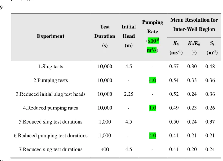
To compare the spatial resolution fields of the two tomography experiments, Figures 4a and 4b 312
show the diagonal elements of the resolution matrix at the corresponding parameter grid cells for 313
experiments with slug tests and pumping tests, respectively. Mean resolution values for cells 314
within the inter-well region are also presented in Table 2 for this comparison. We note that this 315
resolution analysis is based on the 10,000 s records of head or drawdown, which correspond to 316
the termination of each slug test or to the time to reach steady-state conditions. Figures 4a and 4b 317
thus show that independently of the test initiation method, resolutions for Kh, Kv/Kh and Ss are
318
strongly focused on the stressed and observation wells with higher resolutions near the stressed 319
well where sensitivities are larger. This agree with previous studies using both kind of tests 320
(Vasco et al., 1997; Bohling, 2009; Paradis et al., 2015). Moreover, we see that resolution fields 321
for Kh in Figures 4a and 4b are almost identical for the two experiments, as also expressed by
322
similarmean resolution values (Experiments 1 and 2 in Table 2). Mean resolution values are also 323
similar for Kv/Kh despite resolutions that appear much higher near the pumping well, whereas
324
resolutions for Ss are definitely much lower for pumping than for slug tests.
325 326
Explanation of those similarities in parameter resolution can be found in Figures 5a, 5b and 5c. 327
In Figure 5a, we plot as a reference the stressed interval responses for the equivalent slug and 328
pumping tests, as previously discussed. In Figures 5b and 5c, we see that while drawdown due to 329
pumping in the observation interval is three times larger than the head change induced by the 330
slug test, the magnitude of the sensitivity for each hydraulic property is quite similar. Thus, 331
assuming that correlation between sensitivity for each hydraulic property is almost identical for 332
the two tests, comparable parameter resolutions are explained by the similarity in sensitivity 333
magnitudes. Then, head changes due to slug tests are more efficient than drawdowns produced 334
by pumping tests at resolving parameters, as head changes much lower than drawdowns produce 335
similar sensitivity magnitudes. This is due to the sharper form of the head perturbation caused by 336
the instantaneous slug of water applied in the stressed interval that produces larger spatial and 337
temporal hydraulic gradients. Also, this explain why Ss is lower for pumping tests because
338 4 5 6 7 8 9 10 11 12 13 14 15 16 17 18 19 20 21 22 23 24 25 26 27 28 29 30 31 32 33 34 35 36 37 38 39 40 41 42 43 44 45 46 47 48 49 50 51 52 53 54 55 56 57 58 59 60
temporal hydraulic gradients are smaller with pumping, which can be deduced from Figure 5c 339
with Ss sensitivities for pumping about the third of the sensitivities for slug tests.
340 341 Table 2 342 343 Figure 4 344 345 Figure 5 346
4.2 Effect of reduced test stresses
347In this section, we first illustrate the effects of reducing the pumping rate of each pumping test 348
used for the tomography experiment. Indeed, as pumping tests use much more water than 349
equivalent slug tests, such a reduction would be desirable at sites where the storage or injection 350
of a large volume of water may be an issue (e.g., contaminated sites). For our previous 351
tomography experiment, we used 9 L of water to initiate each slug test, whereas 400 L per 352
pumping test was needed to reach steady-state conditions. We note that pneumatic slug test 353
initiation method using air pressure to lower or raise the water level in the stressed interval could 354
also be chosen to avoid using water at sensitive sites. Because a pumping test that would use 355
only 9 L of water would produce non-significant drawdown in the observation intervals, we 356
rather reduce pumping rates by four (experiment 4 in Table 2); thus 100 L of water is used 357
instead of 400 L. We note that at this reduced rate, the peak head from the original slug test and 358
steady-state drawdown of the 100 L pumping test recorded in the stressed intervals have the 359
same magnitudes (Figure 6a). 360
361
As expected from the previous section, Figure 6b shows that reduced pumping rates decrease 362
sensitivity magnitudes, which results in lower parameter resolutions as depicted in Table 2 363
(Experiment 4). Note that reducing initial heads by half leads to a similar decrease in resolutions 364
for tomographic slug tests (Experiment 3 in Table 2). For those particular cases, the effect of 365
reduced initial heads with respect to pumping rates is more pronounced (half the initial heads for 366
a quarter of the original pumping rates) likely due to the head in the observation intervals that are 367
closer to the level of noise, which increases parameter sensitivity correlations. 368 4 5 6 7 8 9 10 11 12 13 14 15 16 17 18 19 20 21 22 23 24 25 26 27 28 29 30 31 32 33 34 35 36 37 38 39 40 41 42 43 44 45 46 47 48 49 50 51 52 53 54 55 56 57 58 59 60 61
369
Figure 6 370
4.3 Effect of reduced test durations
371In this section, we discuss the effects of reducing test durations of both slug tests and pumping 372
tests in order to reduce data acquisition time of tomographic experiments that by design required 373
numerous tests. For our previous synthetic experiment with pumping tests, each test in the field 374
required as much as 2.75 h (10,000 s) to reach steady-state drawdown in the observation 375
intervals. By considering that after each pumping test a recovery period equivalent to the 376
pumping period is needed before conducting the next test, the 13 tests of this experiment would 377
require more than 72 h of testing in the field. For those simulations, we consider recording head 378
and drawdown for each test for a period of 1,000 s (17 min) instead of 10,000 s (2.75 h) (Figure 379
7a), which is considered more realistic for actual field applications. 380
381
As shown in Table 2 (Experiments 5 and 6), both experiments with slug tests and pumping tests 382
see a reduction in resolutions. Examination of Figure 7b suggests that reduced test durations 383
increase sensitivity correlations. In particular, we see that the sensitivity curves for Kv/Kh, and Ss
384
of the pumping test are pretty similar for much of the duration of the test, which implies that 385
their individual effect on drawdown cannot be resolved separately. Moreover, we see in Table 2 386
that the reduction in resolution is more severe with pumping because drawdown at 1,000 s are far 387
from steady-state and still provide important information on parameters, whereas heads related to 388
slug tests are close to their equilibrium state. Further reducing slug test durations long before 389
heads reach their equilibrium state, at 400 s (7 min) for example (Experiment 7 in Table 2; 390
Figures 7a and 7b), also reduces considerably resolutions to values close to pumping tests at 391
1,000 s. We note that pumping tests are longer due to wellbore storage that delays the aquifer 392
response (see Figures 3c and 3d). 393
394
Figure 7 395
5 Summary and discussion
396 4 5 6 7 8 9 10 11 12 13 14 15 16 17 18 19 20 21 22 23 24 25 26 27 28 29 30 31 32 33 34 35 36 37 38 39 40 41 42 43 44 45 46 47 48 49 50 51 52 53 54 55 56 57 58 59 60
In this study, we assessed test initiation methods (slug and pumping tests) and some related field 397
practices on parameter resolutions of tomography experiments. For this purpose, synthetic 398
tomography experiments and their associated sensitivity matrices were generated using a radial 399
flow model accounting for wellbore storage. The resolution analysis was based on a pseudo-400
inverse analysis of the sensitivity matrix with a noise level representative of field measurements. 401
The main findings of this study are summarized and discussed below. 402
403
1. Parameter resolutions are similar for tomography experiments using equivalent slug tests 404
and pumping tests. Using either slug tests or pumping tests that induce identical initial head
405
and steady-state drawdown in the stressed interval lead to similar mean resolutions in 406
hydraulic properties, except for Ss resolution that is slightly lower with pumping. Also, while
407
there are slight differences, parameter resolution fields of tomography experiments 408
simulated with a noise level representative of field conditions are essentially focused on the 409
stressed and observation wells. Thus, for the two different test initiation methods, the same 410
general limitations apply on the resolution of hydraulic properties because hydraulic tests are 411
more sensitive to hydraulic properties in the immediate vicinity of the wells (Vasco et al., 412
1997). 413
414
2. A slug test is more efficient at resolving parameters for the same magnitude in hydraulic 415
perturbations induced in the observation intervals. For instance, for the same values of head
416
changes due to a slug test and drawdown induced by pumping in observation intervals, a 417
slug test is more efficient at resolving parameters due to the sharper form of the induced 418
head perturbation that produces larger sensitivities. So, in the field, one will try to maximize 419
pumping rates even if the drawdown measured in the observation intervals appears 420
“reasonably large”. That could however be difficult as each pumping rate should be 421
adjusted, generally by a trial-and-error process, according to the hydraulic properties 422
surrounding the tested interval that can vary considerably for heterogeneous aquifer systems. 423
In that respect, slug tests could be easier to perform because the initial head is set 424
independently of the materials surrounding the well. However, large initial heads should be 425
initiated in order to induce head changes in observation intervals that are larger than the 426
noise level of the measurements, which may require a slightly more complex testing 427 4 5 6 7 8 9 10 11 12 13 14 15 16 17 18 19 20 21 22 23 24 25 26 27 28 29 30 31 32 33 34 35 36 37 38 39 40 41 42 43 44 45 46 47 48 49 50 51 52 53 54 55 56 57 58 59 60 61
equipment than a single pump (e.g., Paradis et al., 2016). Then, even if large head changes at 428
a distance from a stressed well could be harder to produce with a slug test than drawdowns 429
by pumping, the magnitude of the hydraulic perturbation alone is not a condition sufficient 430
to assess the resolution potential of a tomographic experiment, and the sensitivities 431
associated with each type of test should also be considered. 432
433
3. Wellbore storage leads to the refutation of the principle of reciprocity for both slug tests and 434
transient responses of pumping tests in wells with large diameters. As a consequence of the
435
non-applicability of the principle of reciprocity shown by synthetic experiments, the 436
observation interval response does not provide a unique description of the heterogeneity 437
because it is impossible to tell from this response whether the head change or the drawdown 438
observed result from the flow rate induced by the test at the stressed interval, which is 439
controlled by the surrounding heterogeneity, or the heterogeneity travelled by the hydraulic 440
perturbation to the observation interval location. To obtain this information, stressed and 441
observation interval responses for each test must be recorded in the field and used in the 442
tomographic analysis to isolate the influence of the stressed interval response. Reciprocal 443
tests using only observation interval responses could also be considered, but this alternative 444
is less efficient as it requires twice the number of tests per tomographic experiment. From a 445
practical perspective, head changes in stressed intervals caused by slug tests are generally 446
easier to record with accuracy than drawdown due to pumping that are often influenced by 447
pumping rate variations associated to the equipment itself. Large pumping rates can also 448
induce important head losses in the stressed interval, which should be carefully considered 449
in the analysis to avoid misinterpretation of the recorded water levels. Finally, it should be 450
noted that using stressed and observation interval responses is also important to get better 451
parameter resolutions as the different temporal sensitivity patterns for the different intervals 452
contribute to decrease sensitivity correlations (Paradis et al., 2015). 453
454
4. Reduced test durations produce lower resolutions regardless of the test initiation methods. 455
This finding implies that the recording of slug tests until heads have recovered their initial 456
levels or pumping tests until steady-state is reached should be the preferred practice. 457
However, this practice increases the overall acquisition time of tomography data. In this 458 4 5 6 7 8 9 10 11 12 13 14 15 16 17 18 19 20 21 22 23 24 25 26 27 28 29 30 31 32 33 34 35 36 37 38 39 40 41 42 43 44 45 46 47 48 49 50 51 52 53 54 55 56 57 58 59 60
regard, a slug test offers an important advantage over a pumping test for tomography 459
experiments that generally need many tests since it requires less time per test. For the 460
synthetic tomography experiments discussed in this paper, each slug test requires less than 461
one-third of the time of a pumping test for the same hydrogeological conditions. 462
Furthermore, since slug tests do not require a recovery period (heads are back to their initial 463
levels) before testing the next interval as required after each pumping test, we estimate that 464
an equivalent tomography experiment with slug tests is approximately seven times shorter to 465
carry out in the field than an experiment with the same number of pumping tests. 466
467
Overall, this study demonstrates that tomographic slug tests are an interesting alternative to more 468
commonly used tomographic pumping tests. Indeed, the same level of parameter resolutions 469
could be achieved for a much shorter field effort. This means, that this could foster the use of 470
hydraulic tomography by a larger community of scientists or practitioners outside of the current 471
research community. For future work it would be interesting to assess resolutions and field-472
efficiency of periodic pumping tests and slug tests as proposed by Cardiff et al. (2013) and 473
Guiltinan and Becker (2015), respectively. 474
6 Acknowledgements
475
This study was supported by the Geological Survey of Canada as part of the Groundwater 476
Geoscience Program and by NSERC Discovery Grants held by R.L. and E.G. The authors would 477
like to thank the four anonymous reviewers that provided constructive reviews. This is ESS 478
contribution number 20150440. 479
7 References
480
Aster R C, Borchers B, Thurber C H (2005) Parameter Estimation and Inverse Problems. 301pp 481
Elsevier Amsterdam 482
Berg S J, Illman W A (2011) Three-dimensional transient hydraulic tomography in a highly 483
heterogeneous glaciofluvial aquifer-aquitard system. Water Resour Res 47:W10507 doi: 484 10.1029/2011WR010616 485 4 5 6 7 8 9 10 11 12 13 14 15 16 17 18 19 20 21 22 23 24 25 26 27 28 29 30 31 32 33 34 35 36 37 38 39 40 41 42 43 44 45 46 47 48 49 50 51 52 53 54 55 56 57 58 59 60 61
Berg S J, Illman W A (2013) Field study of subsurface heterogeneity with steady state hydraulic 486
tomography. Groundwater 51(1):29-40 doi:10.1111/j.1745–6584.2012.00914.x 487
Berg S J, Illman W A (2015) Comparison of hydraulic tomography with traditional methods at a 488
highly heterogeneous site. Groundwater 53(1):71-89 doi:10.1111/gwat.12159 489
Bohling G C (2009) Sensitivity and resolution of tomographic pumping tests in an alluvial 490
aquifer. Water Resour Res 45: W02420, 10.1029/2008WR007249 491
Bohling G C, Butler Jr J J (2001) Lr2dinv: A finite-difference model for inverse analysis of two-492
dimensional linear or radial groundwater flow. Comput Geosci 27:1147-1156 493
Bohling G C, Butler Jr J J (2010) Inherent limitations of hydraulic tomography. Ground Water 494
48:809-824 doi:10.1111/j.1745-6584.2010.00757.x 495
Bohling G C, Butler Jr J J, Zhan X, Knoll M D (2007) A Field Assessment of the value of 496
steady-shape hydraulic tomography for characterization of aquifer heterogeneities. Water Resour 497
Res 43(5) W05430 : doi:10.1029/2006WR004932 498
Bohling G C, Zhan X, Butler Jr J J, Zheng L (2002) Steady shape analysis of tomographic 499
pumping tests for characterization of aquifer heterogeneities. Water Resour Res 38(12) 500
1324:doi:10.1029/2001WR001176 501
Butler Jr J J, McElwee C D, Bohling G C (1999) Pumping tests in networks of multilevel 502
sampling wells: Motivation and methodology. Water Resour Res 35(11):3553-3560 503
doi:10.1029/1999WR900231 504
Brauchler R, Liedl R, Dietrich P (2003) A travel time based hydraulic tomographic approach. 505
Water Resour Res 39(12) 1370 doi: 10.1029/2003WR002262 506
Brauchler R, Hu R, Vogt T, Al-Halbouni D, Heinrichs T, Ptak T, Sauter M (2010) Cross-well 507
slug interference tests: An effective characterization method for resolving aquifer heterogeneity. 508
J Hydrol 384(1-2):33-45 509
Brauchler, R.; Hu, R.; Dietrich, P.; et al. (2011) A field assessment of high-resolution aquifer 510
characterization based on hydraulic travel time and hydraulic attenuation tomography. Water 511
Resour Res 47 W03503 512
Brauchler R, Hu R, Hu L, Jiménez S, Bayer P. Dietrich P, Ptak T (2013) Rapid field application 513
of hydraulic tomography for resolving aquifer heterogeneity in unconsolidated sediments Water 514 Resour Res 49(4):2013-2024 515 4 5 6 7 8 9 10 11 12 13 14 15 16 17 18 19 20 21 22 23 24 25 26 27 28 29 30 31 32 33 34 35 36 37 38 39 40 41 42 43 44 45 46 47 48 49 50 51 52 53 54 55 56 57 58 59 60
Butler Jr J J (2005) Hydrogeological methods for estimation of hydraulic conductivity. Edited by 516
Y Rubin Y, Hubbard S in Hydrogeophysics pp 23-58 Springer New York 517
Butler Jr J J, McElwee C D (1990) Variable-rate pumping tests for radially symmetric 518
nonuniform aquifers. Water Resour Res 26(2):291-306 519
Butler Jr J J, McElwee C D (1995) Well-testing methodology for characterizing heterogeneities 520
in alluvial-aquifer systems: Final technical report. Kans Geol Surv Open File Report no 75-95 521
Caers J (2005) Petroleum Geostatistics. 88 p Soc of Pet Eng, Richardson, Tex 522
Cardiff M, Barrash W (2011) 3-D transient hydraulic tomography in unconfined aquifers with 523
fast drainage response. Water Resour Res 47:W12518 doi:10.1029/2010WR010367 524
Cardiff M, Barrash W, Kitanidis P K (2012) A field proof-of-concept of aquifer imaging using 3-525
D transient hydraulic tomography with modular, temporarily-emplaced equipment. Water Resour 526
Res 48:W05531 doi:10.1029/2011WR011704 527
Cardiff M, Bakhos T, Kitanidis P K, Barrash W (2013) Aquifer heterogeneity characterization 528
with oscillatory pumping: Sensitivity analysis and imaging potential. Water Resour Res 529
49(9):5395-5410 530
Cardiff M, Barrash W, Kitanidis P K, Malama B, Revil A, Straface S, Rizzo E (2009) A 531
potential-based inversion of unconfined steady-state hydraulic tomography. Ground Water 532
47(2):259-270 doi:10.1111/j.1745–6584.2008.00541.x 533
Carrera J, Neuman S P (1986) Estimation of aquifer parameters under transient and steady state 534
conditions: 1. Maximum likelihood method incorporating prior information. Water Resour Res 535
22(2):199-210 doi:10.1029/WR022i002p00199 536
Carrera J, Alcolea A, Medina A, Hidalgo J, Slooten L J (2005) Inverse problem in hydrogeology. 537
Hydrogeol J 13:206-222 doi: 10.1007/s10040-004-0404-7 538
Clemo T, Michaels P, Lehman R M (2003) Transmissivity resolution obtained from the 539
inversion of transient and pseudo-steady drawdown measurements. in Proceedings of 540
MODFLOW and More 2003 Understanding Through Modeling p 629-633, Int Ground Water 541
Model Cent, Golden CO USA 542
Doherty J (2003) Ground water model calibration using pilot points and regularization. Ground 543
Water 41(2) :170-177 doi:10.1111/j.1745– 6584.2003.tb02580.x 544
Dougherty D E, Babu D K (1984) Flow to a Partially Penetrating Well in a Double-Porosity 545
Reservoir. Water Resour Res 20(8):1116-1122 doi:10.1029/WR020i008p01116 546 4 5 6 7 8 9 10 11 12 13 14 15 16 17 18 19 20 21 22 23 24 25 26 27 28 29 30 31 32 33 34 35 36 37 38 39 40 41 42 43 44 45 46 47 48 49 50 51 52 53 54 55 56 57 58 59 60 61
Ferris J G, Knowles D B (1963) The slug-injection test for estimating the coefficient of 547
transmissibility of an aquifer. In: US Geological Survey Water-Supply Paper 15361-I, R. Bentall 548
(compiler), p. 299. 549
Fienen M N, Clemo T, Kitanids P K (2008) An interactive Bayesian geostatistical inverse 550
protocol for hydraulic tomography. Water Resour Res 44:W00B01 doi:10.1029/2007WR006730 551
Guiltinan E, Becker M W (2015) Measuring well hydraulic connectivity in fractured bedrock 552
using periodic slug tests. J Hydrol 521 :100-107 doi: 10.1016/j.jhydrol.2014.11.066 553
Gottlieb J, Dietrich P (1995) Identification of the permeability distribution in soil by hydraulic 554
tomography. Inverse Probl 11:353-360 doi:10.1088/0266–5611/11/2/005 555
Huang, S.-Y., J.-C. Wen, T.-C. J. Yeh, W. Lu, H.-L. Juan, C.-M. Tseng, J.-H. Lee, and K.-C. 556
Chang S Y (2011) Robustness of joint interpretation of sequential pumping tests: Numerical and 557
field experiments. Water Resour Res 47:W10530, doi:10.1029/ 2011WR010698 558
Illman W A, Craig A J, Liu X (2008) Practical issues in imaging hydraulic conductivity through 559
hydraulic tomography. Ground Water 46(1) :120-132 doi:10.1111/j.1745-6584.2007.00374.x. 560
Illman W A, Liu X, Craig A (2007) Steady-state hydraulic tomography in a laboratory aquifer 561
with deterministic heterogeneity: Multimethod and multiscale validation of hydraulic 562
conductivity tomograms. J Hydrol 341(3-4) :222-234 doi:10.1016/j.jhydrol.2007.05.011 563
Illman W A, Liu X, Takeuchi S, Yeh T J, Ando K, Saegusa H (2009) Hydraulic tomography in 564
fractured granite: Mizunami underground research site, Japan. Water Resour Res 45:W01406 565
doi:10.1029/2007WR006715 566
Kitanidis, P K (1995) Quasi-linear geostatistical theory for inversing. Water Resour Res 31(10): 567
2411–2419 568
Kruseman G P, de Ridder N A (2000) Analysis and evaluation of pumping test data. ILRI 569
Publishing Netherlands 377pp 570
Leven C, Dietrich P (2006) What information we get from pumping tests? Comparing pumping 571
configurations using sensitivity coefficients. J Hydrol 319:199-215 572
Liu, X, Kitanidis P K (2011) Large-scale inverse modeling with an application in hydraulic 573
tomography. Water Resour Res 47 W02501 doi:10.1029/2010WR009144 574
McElwee C D, Yukler M A (1978) Sensitivity of groundwater models with respect to variations 575
in transmissivity and storage. Water Resour Res 14(3):451-459 doi:10.1029/WR014i003p00451 576 4 5 6 7 8 9 10 11 12 13 14 15 16 17 18 19 20 21 22 23 24 25 26 27 28 29 30 31 32 33 34 35 36 37 38 39 40 41 42 43 44 45 46 47 48 49 50 51 52 53 54 55 56 57 58 59 60
McKinley R M, Vela S, Carlton L A (1968), A field application of pulse-testing for detailed 577
reservoir description. J Petrol Tech 20(3):313-321 578
Menke W (2012) Geophysical Data Analysis: Discrete Inverse Theory. 3rd ed. 293pp Academic 579
Press 580
Moore E H (1920) On the reciprocal of the general algebraic matrix. Bull Am Math Soc 26:394-581
395 582
Novakowski K S (1989) Analysis of pulse interference tests. Water Resour Res 25(11):2377-583
2387 584
Oliver D S (1993) The influence of nonuniform transmissivity and storativity on drawdown. 585
Water Resour Res 29(1):169-178 586
Paradis D, Gloaguen E, Lefebvre R, Giroux B (2015) Resolution analysis of tomographic slug 587
tests head data: Two-dimensional radial case. Water Resour Res 51:2356-2376 588
doi:10.1002/2013WR014785 589
Paradis, D., E. Gloaguen, R. Lefebvre, and B. Giroux (2016) A field proof-of-concept of 590
tomographic slug tests in an anisotropic littoral aquifer. J Hydrol 536:61-73 591
http://dx.doi.org/10.1016/j.jhydrol.2016.02.041 592
Penrose, R (1955) A generalized inverse for matrices. Proc Cambridge Philos Soc 51:406-413 593
Peres, A M, Onur M, Reynolds A C (1989) A new analysis procedure for determining aquifer 594
properties from slug test data. Water Resour Res 25(7):1591-1602 595
Rovey C W, Cherkauer II D S (1995) Scale dependency of hydraulic conductivity 596
measurements. Ground Water 33(5):769-780 597
Rubin, Y, Hubbard S S (2005) Hydrogeophysics. 523 p Springer, Dordrecht, Netherlands 598
Sageev, A (1986) Slug test analysis. Water Resour Res 22(8):1323-1333 599
Soueid Ahmed, S A, Jardani, A, Revil A. Dupont J P (2014) Hydraulic conductivity field 600
characterization from the joint inversion of hydraulic heads and self-potential data. Water Resour 601
Res 50:3502-3522 doi:10.1002/2013WR014645 602
Sun R, Yeh T-C J, Mao D, Jin M, Lu W, Hao Y (2013) A temporal sampling strategy for 603
hydraulic tomography analysis. Water Resour Res 49:3881-3896 doi:10.1002/wrcr.20337 604
Tikhonov, A N (1963) Regularization of incorrectly posed problems. Sov Math Dokl 4(6):1624-605 1627 606 4 5 6 7 8 9 10 11 12 13 14 15 16 17 18 19 20 21 22 23 24 25 26 27 28 29 30 31 32 33 34 35 36 37 38 39 40 41 42 43 44 45 46 47 48 49 50 51 52 53 54 55 56 57 58 59 60 61
Tikhonov, A N, Arsenin V A (1977) Solution of Ill-Posed Problems. 258 p., John Wiley New-607
York 608
Tonkin, M J, Doherty J (2005) A hybrid regularization methodology for highly parameterized 609
environmental models. Water Resour Res 41 W10412 doi:10.1029/2005WR003995 610
Tosaka H, Masumoto K, Kojima K (1993) Hydropulse tomography for identifying 3-D 611
permeability distribution in high level radioactive waste management. Proceedings of the Fourth 612
Annual International Conference of the ASCE, pp. 955-959, Am. Soc. Civ. Eng., Reston, Va. 613
Vasco D W, Datta-Gupta A, Long J C S (1997) Resolution and uncertainty in hydrologic 614
characterization. Water Resour Res 33(3):379-397 doi:10.1029/96WR03301 615
Xiang, J, Yeh T-C J, Lee C-H, Hsu K-C, Wen J-C (2009) A simultaneous successive linear 616
estimator and a guide for hydraulic tomography analysis. Water Resour Res 45 W02432 617
doi:10.1029/2008WR007180 618
Yeh T-C J, Liu S (2000) Hydraulic tomography: Development of a new aquifer test method. 619
Water Resour Res 36 (8):2095-2105 doi:10.1029/2000WR900114 620
Zha, Y, Yeh T-C J, Mao D, Yang J, Lu W (2014) Usefulness of flux measurements during 621
hydraulic tomographic survey for mapping hydraulic conductivity distribution in a fractured 622
medium. Adv Water Resour 71:162-176 doi:10.1016/j.advwatres.2014.06.008 623
Zhu J, Yeh T-C J (2005) Characterization of aquifer heterogeneity using transient hydraulic 624
tomography. Water Resour Res 41:W07028 doi:10.1029/2004WR003790 625 626 627 628 4 5 6 7 8 9 10 11 12 13 14 15 16 17 18 19 20 21 22 23 24 25 26 27 28 29 30 31 32 33 34 35 36 37 38 39 40 41 42 43 44 45 46 47 48 49 50 51 52 53 54 55 56 57 58 59 60
Tomographic Slug and Pumping Tests Comparison 1/2 Figures Captions
1 2
Figure 1. Schematic diagram illustrating the general approach used for the evaluation of the
3
resolution matrix of a tomography experiment. 1) Starting from an idealized aquifer system and a 4
test configuration, sensitivities are calculated using the numerical flow simulator through a 5
perturbation approach. 2) A Moore-Penrose pseudo-inverse approach is then applied on the 6
resulting sensitivity matrix to evaluate the associated resolution matrix. 3) Resolution 7
characteristics of the tomography experiment is finally analyzed through inspection of the 8
diagonal elements of the resolution matrix. 9
10
Figure 2. Head and drawdown for reciprocal slug tests and pumping tests, respectively, for the
11
case with a test configuration symmetrical with respect to layering in Kh, Kv and Ss. (a) Aquifer
12
model and test configuration; (b) Head for reciprocal slug tests; (c) Drawdown for reciprocal 13
pumping tests considering wellbore storage in the stressed well; and (d) Drawdown for 14
reciprocal pumping tests neglecting wellbore storage in the stressed interval. Note that reciprocal 15
tests are simulated by mirroring the vertical locations of the stressed and observation intervals to 16
represent the two different testing directions. Values of Kh, Kv and Ss for the different simulations
17
are compiled in Table 1. 18
19
Figure 3. Head and drawdown for reciprocal slug tests and pumping tests, respectively, for the
20
case with a test configuration asymmetrical with respect to layering in Kh, Kv and Ss. (a) Aquifer
21
model and test configuration; (b) Head for reciprocal slug tests; (c) Drawdown for reciprocal 22
pumping tests considering wellbore storage in the stressed well; and (d) Drawdown for 23
reciprocal pumping tests neglecting wellbore storage in the stressed interval. Note that reciprocal 24
tests are simulated by mirroring the vertical locations of the stressed and observation intervals to 25
represent the two different testing directions.Values of Kh, Kv and Ss for the different simulations
26
are compiled in Table 1. 27
28
Figure 4. Diagonal elements of the resolution matrix for Kh, Kv/Kh, and Ss associated with the
29
analysis of the synthetic 10,000 s head (a) and drawdown (b) records for a homogeneous and 30
anisotropic model. Resolutions are based on a Moore-Penrose pseudo-inverse of the sensitivity 31
matrix for a relative parameter error of 10% and a random noise with a standard deviation of 32
2x10⁻⁴ m (see Supplementary Material for supportive information). 33
34
Figure 5. Head and drawdown in (a) stressed and (b) observation intervals for a single test.
35
Sensitivities in Kh, Kv/Kh, and Ss for the observation interval in (c) are computed for the entire
36
inter-well region. Stressed and observation intervals are located in the middle of the wells. 37
38
Figure 6. (a) Head and drawdown as well as (b) sensitivities in Kh, Kv/Kh, and Ss for the
39
observation interval of a single test considering a reduced pumping rate of 1.0x10⁻⁵ m3/s (0.6 40
LPM). Head and sensitivities for the slug test in gray are from Figure 5 for reference. Head and 41
sensitivities for reduced initial slug test head of 2.25 m (Table 2) are not shown, but their 42
magnitudes are half those of Figure 5 (gray lines). 43
44
Figure 7. (a) Head and drawdown as well as (b) sensitivities in Kh, Kv/Kh, and Ss for the
45
observation interval of a single test considering a reduced test duration lasting 1,000 s instead of 46
10,000 s. 47
Observation Well Stressed Well Observation Well Stressed Well Numerical Model Sensitivity Matrix Resolution Matrix 1. Sensitivity Computation 2. Moore-Penrose Pseudo-Inverse m: number of measurements n: number of parameters J 11 ... J1n ... ... ... Jm1 ... Jmn m n n n R 11 ... R1n ... ... ... Rn1 ... Rn n Tomographic Experiment ... ... ... 1 2 3 4 5 6 7 8 9 10 11 12 13 3. Resolution Matrix
Analysis Diagonal Elements
+
ObservationIntervals
Stressed Interval
100101102103104105 0 1 2 3 4 5 6 Time (sec) D ra w d o w n (m)-St re s. 100101102103104105 0 1 2 3 4 5 6 Time (sec) 100101102103104105 0 1 2 3 4 5 6 Time (sec) D ra w d o w n (m)-O b s. 0 0.1 0.2 0.3 0.4 0.5 0.6 (A) Symmetrical reciprocal test configuration with respect to heterogeneity
El e va ti o n (m) 2 4 6 8 10 12 14 16 18 6 4 2 Distance (m) well 1 well 2 0 0 8 Unchanged Unchanged Kh, Kv or Ss Varied (B) Slug tests 0 0.05 0.1 100 101 102 103 104 0 1 2 3 4 5 Time (sec) H e a d (m)-St re s. 100 101 102 103 104 0 1 2 3 4 5 Time (sec) H e a d (m)-O b s. 100 101 102 103 104 0 1 2 3 4 5 Time (sec) Kv varied Ss varied Kh varied well 1 well 2 well 1 well 2 100101102103104105 0 1 2 3 4 5 6 Time (sec) D ra w d o w n (m)-St re s. 100101102103104105 0 1 2 3 4 5 6 Time (sec) 100101102103104105 0 1 2 3 4 5 6 Time (sec) D ra w d o w n (m)-O b s. 0 0.1 0.2 0.3 0.4 0.5 0.6 (C) Pumping tests considering wellbore storage
(D) Pumping tests without wellbore storage
1 2 3 Kv varied Ss varied Kh varied Kv varied Ss varied Kh varied stres. obs. stres. obs. stres. obs. stres. obs. stres. obs. stres. obs. stres. obs. stres. obs. stres. obs.
100101102103104105 0 1 2 3 4 5 6 Time (sec) D ra w d o w n (m)-St re s. 100101102103104105 0 1 2 3 4 5 6 Time (sec) 100101102103104105 0 1 2 3 4 5 6 Time (sec) D ra w d o w n (m)-O b s. 0 0.1 0.2 0.3 0.4 0.5 0.6 100101102103104105 0 1 2 3 4 5 6 Time (sec) D ra w d o w n (m)-St re s. 100101102103104105 0 1 2 3 4 5 6 Time (sec) 100101102103104105 0 1 2 3 4 5 6 Time (sec) D ra w d o w n (m)-O b s. 0 0.1 0.2 0.3 0.4 0.5 0.6 0 0.05 0.1 100 101 102 103 104 0 1 2 3 4 5 Time (sec) H e a d (m)-St re s. 100 101 102 103 104 0 1 2 3 4 5 Time (sec) H e a d (m)-O b s. 100 101 102 103 104 0 1 2 3 4 5 Time (sec)
(A) Asymmetrical reciprocal test configuration with respect to heterogeneity
El e va ti o n (m) 2 4 6 8 10 12 14 16 18 6 4 2 Distance (m) well 1 well 2 0 0 8 (B) Slug tests well 1 well 2 well 1 well 2
(C) Pumping tests considering wellbore storage
(D) Pumping tests without wellbore storage
Unchanged Kh, Kv or Ss Varied 1 2 Kv varied Ss varied Kh varied Kv varied Ss varied Kh varied Kv varied Ss varied Kh varied stres. obs. stres. obs. stres. obs. stres. obs. stres. obs. stres. obs. stres. obs. stres. obs. stres. obs.
(A) El e va ti o n (m)
Slug: 10000 sec, Kh Resolution
2 4 6 8 10 12 14 16 18 6 4 2 0 0.2 0.4 0.6 0.8 1 El e va ti o n (m)
Slug: 10000 sec, Kv/Kh Resolution
2 4 6 8 10 12 14 16 18 6 4 2 0 0.2 0.4 0.6 0.8 1 Distance (m) El e va ti o n (m)
Slug: 10000 sec, Ss Resolution
2 4 6 8 10 12 14 16 18 6 4 2 0 0.2 0.4 0.6 0.8 1 str. obs. (B) El e va ti o n (m)
Pumping: 10000 sec, Kh Resolution
2 4 6 8 10 12 14 16 18 6 4 2 0 0.2 0.4 0.6 0.8 1 El e va ti o n (m)
Pumping: 10000 sec, Kv/Kh Resolution
2 4 6 8 10 12 14 16 18 6 4 2 0 0.2 0.4 0.6 0.8 1 Distance (m) El e va ti o n (m)
Pumping: 10000 sec, Ss Resolution
2 4 6 8 10 12 14 16 18 6 4 2 0 0.2 0.4 0.6 0.8 1 str. obs.
4 10 101 102 103 10 Time (sec) 0 0 1 2 3 4 5 H e a d /D ra w d o w (m) Drawdown Head Stressed Interval -0.04 -0.02 0 0.02 0.04 No rma lize d se n si tivi ty (m) Kh Kv/Kh Ss Observation Interval Observation Interval 4 10 101 102 103 10 Time (sec) 0 0.1 0.2 0.3 0 H e a d /D ra w d o w n (m) 4 10 101 102 103 10 Time (sec) 0 (A) (B) (C) Head from slug test Drawdown from pumping test Pumping Slug
Steady-state drawdown from pumping Peak head from Figure 5b Observation Interval 4 10 101 102 103 10 Time (sec) 0 0.1 0.2 0.3 0 H e a d /D ra w d o w n (m) Kh Kv/Kh Ss -0.04 -0.02 0 0.02 0.04 No rma lize d se n si tivi ty (m) 4 10 101 102 103 10 Time (sec) 0 Observation Interval (A) (B) Pumping Slug (from Figure 5c)
-0.04 -0.02 0 0.02 0.04 No rma lize d se n si tivi ty (m) Kh Kv/Kh Ss Observation Interval Observation Interval 4 10 101 102 103 10 Time (sec) 0 0.1 0.2 0.3 0 H e a d /D ra w d o w n (m) 4 10 101 102 103 10 Time (sec) 0 (A) (B) 17 min 7 min 2.5 h 17 min 7 min 2.5 h Head from slug test Drawdown from pumping test Pumping Slug
Tomographic Slug and Pumping Tests Comparison 1/2
Table 1. Hydraulic properties of each layer in the model used for the verification of the principle
1
of reciprocity for slug tests and pumping tests. 2 3 Simulation Layer Kh (ms-1) Kv (ms-1) Ss (m-1) Kh varied 2 1x10⁻⁶ 1x10⁻⁶ 1x10⁻⁵ Kv varied 2 1x10⁻⁵ 1x10⁻⁵ 1x10⁻⁵ Ss varied 2 1x10⁻⁵ 1x10⁻⁶ 1x10⁻⁶
For all simulations 1 and 3 1x10⁻⁵ 1x10⁻⁶ 1x10⁻⁵ 4