A Comparison of Nonlinear Mixing Models for Vegetated Areas Using Simulated and Real Hyperspectral Data

To link to this article : doi:10.1109/JSTARS.2014.2328872

URL :

http://dx.doi.org/10.1109/JSTARS.2014.2328872

Open Archive TOULOUSE Archive Ouverte (OATAO)

OATAO is an open access repository that collects the work of Toulouse researchers and

makes it freely available over the web where possible.

This is an author-deposited version published in :

http://oatao.univ-toulouse.fr/

Eprints ID : 11938

To cite this version : Dobigeon, Nicolas and Tits, Laurent and Somers,

Ben and Altmann, Yoann and Coppin, Pol A Comparison of Nonlinear

Mixing Models for Vegetated Areas Using Simulated and Real

Hyperspectral Data. (2014) IEEE Journal of Selected Topics in Applied

Earth Observations and Remote Sensing, vol. 7 (n° 6). pp. 1869-1878.

ISSN 1939-1404

Any correspondance concerning this service should be sent to the repository

administrator:

staff-oatao@listes-diff.inp-toulouse.fr

A Comparison of Nonlinear Mixing Models for

Vegetated Areas Using Simulated and Real

Hyperspectral Data

Nicolas Dobigeon, Senior Member, IEEE, Laurent Tits, Ben Somers, Yoann Altmann, Member, IEEE, and Pol Coppin

Abstract—Spectral unmixing (SU) is a crucial processing step when analyzing hyperspectral data. In such analysis, most of the work in the literature relies on the widely acknowledged linear mixing model to describe the observed pixels. Unfortunately, this model has been shown to be of limited interest for specific scenes, in particular when acquired over vegetated areas. Consequently, in the past few years, several nonlinear mixing models have been introduced to take nonlinear effects into account while performing SU. These models have been proposed empirically, however, with-out any thorough validation. In this paper, the authors take advan-tage of two sets of real and physical-based simulated data to validate the accuracy of various nonlinear models in vegetated areas. These physics-based models, and their corresponding unmixing algo-rithms, are evaluated with respect to their ability of fitting the measured spectra and providing an accurate estimation of the abundance coefficients, considered as the spatial distribution of the materials in each pixel.

Index Terms—Hyperspectral imagery, nonlinear spectral mixtures, ray tracing, spectral unmixing (SU), vegetated areas.

I. INTRODUCTION

S

scene and, for each pixel of the image ( ),

estimating the corresponding proportions (or abundances) that represent the spatial distributions of these materials over the area of interest [1]. The first automated unmixing techniques have been proposed in the early 1990 s [2]. When no prior knowledge is available regarding the studied scene, SU can be usually decomposed into two successive steps: 1) the endmembers are extracted from the image and 2) the proportions of the materials are estimated in the so-called

inversion step. A vast majority of the endmember extraction algorithms (EEAs) and inversion techniques exploit some geo-metrical concepts that are intrinsically related to an assumption of a linear mixing process to explain the observed pixels. In other words, under this linear mixing model (LMM), each observed pixel of a given image is assumed to result from the linear combination of the endmember spectra

where denotes the proportions of the

materials in the th pixel, is the endmember

matrix, and stands for an additive residual term accounting for the measurement noise and modeling error. Since the mixing coefficients are expected to represent the actual spatial distribution of the materials in the th pixel, they are commonly subject to the following positivity and sum-to-one (or additivity) constraints

This LMM has received a considerable attention in the image processing and remote sensing literature since it represents an acceptable first-order approximation of the physical processes involved in most of the scenes of interest [2]. Consequently, it has motivated a lot of research works that aim at developing efficient EEA, designed to recover pure spectral signatures in the image, and inversion techniques to estimate the abundance coefficients for a given (estimated or a priori known) set of endmembers. Comprehensive overviews of these EEA and inversion methods can be found in [1]–[3]. Specifically, two main approaches have been advocated to solve the inversion step, that can be formulated as a constrained optimization problem solved by fully con-strained least square (FCLS) algorithms [4]–[6] or as a statistical estimation problem solved within a Bayesian framework [7]–[9]. However, for specific applications, LMM has demonstrated some difficulties to accurately describe real mixtures [10]. Notably, intimate mixtures of minerals are characterized by spatial scales typically smaller than the path length followed by the photons, which violates one fundamental assumption for considering a linear model. Analyzing such mixtures, e.g., composed of minerals, requires to resort to complex physical models coming from the radiative transfer theory. Various approximating models have been proposed in the spectroscopic

N. Dobigeon and Y. Altmann are with the IRIT/INP-ENSEEIHT/TéSA, University of Toulouse, 31071 Toulouse Cedex 7, France (e-mail: Nicolas. Dobigeon@enseeiht.fr; Yoann.Altmann@enseeiht.fr).

L. Tits and P. Coppin are with the Department of Biosystems, Katholieke Universiteit Leuven, 3001 Leuven, Belgium (e-mail: Laurent.Tits@biw. kuleuven.be; Pol.Coppin@biw.kuleuven.be).

B. Somers is with the Division of Forest, Nature, and Landscape, Katholieke Universiteit Leuven, 3001 Leuven, Belgium (e-mail: ben.somers@ees.kuleuven. be).

literature, such as the popular Hapke’s model [11]. More recently, this model or related alternatives have been exploited in the hyperspectral literature to derive unmixing algorithms dedicated to remotely sensed images [12], [13]. Broadwater and Banerjee derived various kernel-based unmixing techniques that implicitly relied on the Hapke model [14]–[16]. In [17]–[19], Close et al. combined linear and intimate mixing processes in single models to improveflexibility.

Conversely, scenes acquired over vegetated areas are also known to be subjected to more complex interactions that cannot be properly taken into account by a simple LMM [20]–[27]. Indeed, for these specific scenarios addressed in this paper, differences in elevation between the transparent 3D vegetation canopies and the relativelyflat soil surfaces submit photons to multipath and scattering effects. Similar interaction effects have been also encountered when analyzing urban scenes [28]–[30]. Therefore, various attempts have been conducted to overcome the intrinsic limitations of the LMM. A large family of nonlinear models that have been proposed to analyze vegetated areas can be described as

¹

In (3), the observed pixel is composed of a linear contribution similar to the LMM and an additive nonlinear term¹ that may depend on the endmember matrix , the abundance coefficients in , and additional nonlinearity coefficients introduced to adjust the amount of nonlinearity in the pixel. This class of models includes the bilinear models [31], the quadratic–linear model [30], the postnonlinear model [32], and the bilinear– bilinear model [33] (the most commonly used will be fully described in Section II).

However, to our knowledge, most of these models have been derived following physical or intuitive considerations, without any careful and thorough analysis of their ability to properly describe real mixtures while performing SU. In this article, we propose tofill this gap by evaluating the relevance of various nonlinear models when used for SU of images acquired over vegetated areas. Specifically, requirements for ensuring the quality of a model in this specific applicative context are threefold: 1) the model should not depend on external parameters related to the studied scene (e.g., leaf index area, geometry, or illumination incidence) since this prior knowledge is generally not available; 2) this model should be still sufficiently flexible to fit the real observations in various external conditions, despite the ignorance of these unknown external parameters; and 3) it should be able to account for the relative spatial distribution of the materials in the pixel, with the prime objective to estimate the abundance coefficients. In particular, mainly because of the two first requirements enounced above, advanced nonlinear models proposed in the remote sensing literature (e.g., [20]) will not be considered in this study since they need a detailed prior knowl-edge regarding the analyzed scene.

To meet this challenge, we take advantage of an interesting set of simulated and in situ collected hyperspectral data. First, we use a detailed virtual orchard and forest model constructed in a physically based ray-tracing environment using detailed sub-models for the description of tree geometry, leaf and soil bidirectional reflectance, and diffuse illumination [34]–[36].

The model has been thoroughly validated withfield observations [34], and more recently we could provide, based on a comparison with in situ data, strong evidence that our ray tracing model realistically describes the spectral scattering and thus nonlinear-ity observed in vegetated areas [27]. Second, we use data from an in situ experiment in a commercial citrus orchard. This experi-ment comprised in situ measured mixed pixel reflectance spectra, pixel specific endmember spectra and subpixel cover fraction distributions. This unique dataset of in situ measured mixed pixel reflectance spectra has previously been used to study nonlinearity in fruit orchards [25].

The paper is organized as follows. Section II introduces the main nonlinear models that have been proposed in the literature to describe mixtures encountered in vegetated areas. The ray-tracer-based simulated data and the in situ measurements used to validate these models are described in Section III. The experi-ment results obtained by using the previously introduced non-linear models on the two sets of data are reported in Section IV. A comprehensive discussion on these results is conducted in Section V. Section VI concludes the paper.

II. NONLINEARMIXINGMODELS

A. Bilinear Models

To take into account the scattering effects the photons are subjected to before reaching the sensor, a wide class of nonlinear models are derived by defining the nonlinear component ¹ in (3) as a sum of bilinear terms [31]

¹ ≜

where the operator stands for a termwise product

≜

The set of nonlinearity coefficients allows the amount of nonlinearity in the th pixel to be adjusted between each pair of materials and . Most of the various bilinear models of the literature mainly differ by the definition of these coefficients and the associated constraints they are subject to. The most common models, that will be evaluated in Section IV, are recalled below.

The model derived in [37] and [25] proposes to include the nonlinearity coefficients within the set of constraints (2) defined by the LMM, leading to

≜ with

Note that this model, denoted NM for Nascimento’s model in this paper, reduces to the LMM when , . This is an interesting property since the LMM is known to be an admissible first approximation of the actually involved physical processes.1 However, in a more general case (i.e., ), the abundance coefficients are not subject to the sum-to-one con-straints defined in (2).

In [24], Fan et al. have defined the nonlinearity coefficients as the product of the abundances, ≜ , under the LMM-based constraints in (2), leading to the so-called Fan’s model (FM)

≜

The main motivation for relating the amount of nonlinear interactions (governed by ) to the amount of linear contri-bution (governed by and ) is straightforward: the more a given material is present in the pixel, the more nonlinear inter-actions may occur. In particular, if a component is absent in

the th pixel, then and consequently , which

means that there are no interactions between the material and any other materials ( ). Note, however, that this bilinear model does not extend the LMM.

To cope with this latter limitation, the generalized bilinear model (GBM) [38] weights the products of abundances by additional free parameters that tune the amount of nonlinear interactions, leading to ≜ and

≜

The GBM has the nice properties of 1) generalizing the LMM by enforcing ( ), similarly to NM but contrary to FM and 2) having the amount of nonlinear interactions to be proportional to the material abundances, similarly to FM but contrary to NM.

B. Postnonlinear Mixing Model

Inspired by pioneered works in blind source separation [39], Altmann et al. have introduced in [32] a nonlinear model that relies on a second-order polynomial expansion of the nonlinearity

¹ ≜

leading to the following polynomial postnonlinear mixing model (PPNM)

The PPNM has demonstrated a noticeableflexibility to model various nonlinearities not only for unmixing purposes [32] but also to detect nonlinear mixtures in the observed image [40]. This model has also the great advantage of having the amount of nonlinearity to be governed by a unique parameter in each pixel, contrary to NM or GBM. Equation (9) also shows PPNM includes bilinear terms ( ) similar to those in-volved in the NM, FM, and GBM, and also quadratic terms , which may account for interactions between similar materials.

C. Unmixing Algorithms

To evaluate the accuracy of the mixing models of interest, the pixels of the in situ and simulated data are unmixed with respect to each model. When analyzing the pixels with the LMM, the nonlinear contribution¹ is set to zero. Based on the prior knowledge of the endmember signatures , the abundance vector associated with each pixel is estimating by solving the constrained minimization problem

In this work, to solve this problem, the FCLS algorithm [4] is used.

Moreover, when analyzing the pixels with nonlinear mixing models, the abundance vector and the nonlinearity parameter vector associated with each pixel are estimated by solving the following constrained optimization problem

¹

Depending on the considered model, the set of constraints imposed to the abundance vector and the possible nonlinear coefficient vector may differ. For the FM, GBM, and PPNM, the abundance vector should satisfy the LMM-based con-straints (2), while for the NM, this constraint is applied to the joint vector . Similarly, the nonlinear coefficient vector for the GBM and PPNM should satisfy constraints that depend on the considered model and the nonlinearity component ¹

in (4) or (9) depends also on the considered nonlinear model.

For the experimental results reported in Section IV, the FCLS algorithm is used to solve the NM-based unmixing problem since NM can be interpreted as a linear mixture of an extended set of endmembers, as shown in [37]. The FM parameters are estimated with the algorithm detailed in [24], based on afirst-order Taylor series expansion of the nonlinearity¹ . Finally, the gradient descent and the subgradient descend algorithms devel-oped in [41] and [32] are used to solve the GBM- and PPNM-based unmixing problems, respectively. Interested readers are invited to refer to these works for detailed information regarding the optimization schemes.

III. DATADESCRIPTION

The mixing models and corresponding unmixing algorithms detailed in the previous sections are compared using simulated and real hyperspectral images. It is worth noting that, for both 1_{It is widely admitted that the pixel spectrum measured by the sensor can be}

accurately described by the LMM when 1) the photons are not subjected to multipath effects and 2) the materials are arranged side-by-side in the scene (as a checkerboard structure) [2].

kinds of datasets, actual pure component spectral signatures (i.e., endmember spectra) and quantitative spatial distributions of these components (i.e., abundances) are available as ground truth in each pixel of the considered images. These datasets2 are described in this section.

A. Simulated Dataset

Two types of synthetic hyperspectral image data were gener-ated from a ray tracing experiment. First, synthetic but realistic fully calibrated virtual scenes, namely citrus orchards and a forest, have been designed using methods developed in [34] and [42], respectively, which will be explained in more detail in the following paragraphs. Then, corresponding hyperspectral images have been simulated using an extended version of the physically based ray tracer (PBRT) [43]. In PBRT, a scene is defined using submodels to describe the various components of the scene: illumination sources, sensor platform, material optical properties, integrator, and geometry descriptions. For the differ-ent generated images, the illumination has been modeled to closely agree with the average circadian illumination from April until September, corresponding to a midlatitude northern hemisphere growing season. The illumination has been com-posed of a combination of direct and diffuse light calculated from 350 to 2500 nm with a 10 nm interval. The citrus trees and weeds of the orchard scenes (see Section III-A1) and the trees of the forest scene (see Section III-A2) have been con-structed as triangular meshes by implementing the algorithm introduced in [44]. Their material properties have been described by a bidirectional scattering distribution function (BSDF) model [34].

1) Orchard Scenes: The fully calibrated virtual citrus orchard developed in [34] has been used to create two different orchard scenes: 1) an orchard consisting of citrus trees and a soil background, leading to two-endmember mixtures and 2) an orchard consisting of citrus trees, a soil background and weed patches, leading to three-endmember mixtures. Each orchard scene consists of pixels, with a pixel size of . The exact per-pixel abundances are known for the three components, as well as the reference spectral signatures. More precisely, for the soil endmember, the pure spectral signature consisted of the fully sunlit soil uncontaminated by the surrounding trees. For the tree endmember, the soil background of the orchard was replaced by a perfectly absorbing background, to minimize the influence of the background on the tree signature. A 5-cm resolution image of was rendered above a canopy with one row. Only the pixels containing a tree fraction greater than 0.95 were retained and averaged to provide the pure tree signature. As such, the tree spectral signatures are an integration of all components of a tree, including sunlit and shaded leafs, branches, and stems. For the weed endmember spectral signature, a similar approach to the tree endmember was used, replacing the soil background with a perfectly absorbing background, and removing all trees from the orchard. A image with 1-cm resolution was rendered over a

weed patch, selecting only those pixels with a weed fraction greater than 0.95. Finally, these pixels were averaged to provide the spectral signature of the weeds. The resulting endmember spectra are depicted in Fig. 1.

The orchards have been constructed with a row spacing of 4.5 m, tree spacing of 2 m, row azimuth of 7.3 , and an average tree height of 3 m. This composition is consistent with the reference orchard, located in Wellington, South Africa (33.58 , 18.93 ), used to calibrate the virtual orchard [34]. Spectral input data for citrus leaves and stems, soils, and weeds have been measured using a full-range (350–2500 nm) analytic spectral devices (ASDs) Fieldspec JR spectroradiometer with a 25 foreoptic. The weed spectrum has been chosen as of the Lolium sp. A Haplic Arenosol [45] typical for commercial citrus orchards in the Western Cape Province in South Africa has been used in the simulations [46]. An example of a high-resolution image of of the two-endmember orchard is de-picted in Fig. 2(a), while the three-endmember orchard is shown in Fig. 2(b). For a detailed description of the design, modalities, and application of the virtual orchard, the reader is invited to consult [34].

2) Forest Scene: The virtual forest consisted of a soil background planted with trees selected from the species-specific tree pools. More precisely, to simulate the forest scene, 3D tree geometry descriptions were available for beech (Fagus sylvatica L.) and poplar (Populus nigra L. var.“italic” Muench). Each tree was characterized by a specific structure based on its age (i.e., 20 years old). All leaves were assigned a species-specific reflectance and transmittance spectrum extracted from the leaf optical properties experiment (LOPEX) dataset [47]. Examples of the soil, beech, and pop endmember signatures are depicted in Fig. 3.

Fig. 1. Two- and three-endmember orchard synthetic dataset. Endmember spectra: soil (black), weed (red), and tree (green).

Fig. 2. High-resolution images of the two orchards with (a) two endmembers, i.e., tree and soil, and (b) three endmembers, i.e., tree, soil, and weeds.

2

To achieve a nearly 100% canopy cover, the average tree spacing has been set to 5 m for the beech trees and 1 m for the poplars. A series of six forest scenes has been rendered providing a gradual transition from a forest scene completely dominated by one species to a scene dominated by the other species. More precisely, 20% of the beech trees have been randomly replaced by poplar trees in the subsequent scene. Each forest scene

con-sisted of pixels, with a pixel size of .

In Fig. 4, a detail is shown of a 30-m pixel, for the forest consisting of 60% beech trees and 40% poplars. Note here that the spatial resolution of the forest scene is significantly larger than the resolution of the orchard scene detailed in Section III-A1. These choices allow different plant production systems to be covered, with various species combinations, sets of endmembers and spatial resolution scales.

B. In Situ Measurement

In addition, an experiment was conducted in the same orchard used for the calibration of the virtual orchard described in Section III-A1. Significant weed cover, dominantly Lolium sp. L. ( of the inter-row spacing, concentrated in dense patches) was present. Throughout the orchard, in situ measured reflectance spectra of 60 mixed ground plots were collected, i.e., 25 mixtures of tree and soil, 25 mixtures of tree and weed, and 25 mixtures of tree, soil and weed. Reflectance measure-ments were performed in August using a spectroradiometer with

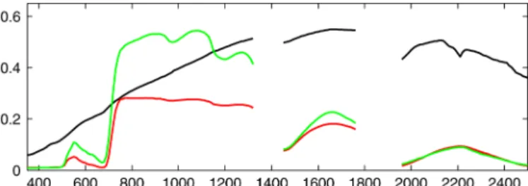
a 25 fore-optic, covering the 350–2500 nm spectral domain (Analytic Spectral Devices, Boulder, CO, USA). The measure-ments were taken from nadir at a height of 4 m. For each measured mixed pixel, the plot-specific pure endmember spectra and ground cover fraction distributions were determined. Specifically, to mitigate the impact of nonlinear mixing from endmember variability, plot-specific endmembers were acquired by measuring a number of pure spectra in each plot, as illustrated in Fig. 5. One set of soil, weed, and tree endmember spectra is depicted in Fig. 6.

Information on the ground cover composition of each of the measured mixed pixels was extracted from digital photographs (SONY DSC-P8/3.2 megapixel cyber shot camera, positioned in nadir). A more detailed description on the experimental setup, depicted in Fig. 5, can be found in [25].

IV. EXPERIMENTALRESULTS

The relevance of the mixing models under test, namely LMM, FM, NM, GBM, and PPNM, and associated unmixing algo-rithms, is evaluated with respect to 1) their ability of accurately describing the physical processes yielding the considered mix-tures and 2) their ability of providing meaningful estimations of the abundance coefficients, to properly account for the spatial distribution of the materials over each observed pixel. More precisely, let and denote the abundance and nonlinearity coefficient vectors estimated by the algorithms introduced in Section II-C. First, the average square reconstruction error (RE) is measured as

where stands for the usual Euclidean norm ( ). In the right-hand side of (13), ( ) are the observed pixels whereas are the corresponding estimates given by

¹

Fig. 3. Forest synthetic dataset. Example of the generated endmember spectra: soil (black), beech (red), and pop (green).

Fig. 4. High-resolution detail of a 30 m pixel of the forest with 60% beech trees and 40% poplars.

Fig. 5. Experimental set-up to determine plot-specific soil and tree endmember signatures for each plot [25]. The areas T1, T2, and T3 (S1, S2, and S3, respectively) identify the subplots selected for the measurements of pure tree (soil) spectra. These measurements are averaged to provide the plot-specific tree (soil) endmember signature.

where¹ is equal to 0 for the LMM or stands for the additional nonlinear contribution for the nonlinear models (see Section II). Since the actual endmember spectra and abundance coeffi-cients [that satisfy the constraints in (2)] are perfectly known for each pixel of the considered scenes, these REs can also be computed from pixels reconstructed following the LMM and FM with the actual values of the abundances. These two“oracle” models are denoted o-LMM and o-FM in what follows. In particular, the RE associated with the o-LMM provides interest-ing information regardinterest-ing the actual level of nonlinearities in the considered pixels. Note also that such oracle performance cannot be computed for the other nonlinear models, since NM is based on a different abundance definition [e.g., they do not follow the constraints (2)] and GBM and PPNM require the prior knowl-edge of additional (unknown) parameters.

Moreover, to visualize the reconstruction error as a function of the wavelength, a signed error, defined as the mean reconstruc-tion difference in the th band, is also computed as

Finally, to measure the accuracy of the abundance estimation, the mean square errors (MSE) between the actual abundance

vectors and the corresponding estimated ( )

are computed as follows:

A. Simulated Dataset

1) Virtual Orchard: The unmixing results for the simulated orchard scenes are shown in Table I in terms of MSE and RE. From these results, for both two- and three-endmembers, one can conclude that NM and LMM perform similarly in term of RE, while PPNM and FM provide the best results and, in particular, significantly better than LMM. It is interesting to note that, for the two-endmember mixtures, GBM does not provide smaller RE than LMM, as expected. Indeed, as highlighted in Section II-A, GBM reduces to LMM if , which is supposed to confer to GBM moreflexibility than LMM. This might indicate that the unmixing algorithm associated with GBM has not properly converged for this dataset. This point is discussed in more details in Section V. Regarding the abundance MSE, NM and LMM provide similar errors for two-endmember mixtures and all nonlinear models perform better than LMM for three-endmember mixtures.

In Fig. 7, the RDs are depicted as functions of wavelength, for the different linear and nonlinear mixing models. From this figure, it appears that the nonlinearities occurring in spectral bands ranging from 1400 to 2500 nm are of high intensity (see the plot associated with the oracle-LMM, in black dashed line) but are rather well described by the various nonlinear models.

2) Virtual Forest: For the simulated forest scenes, the unmixing results are reported in Table II. These results are computed for four scene compositions, with increasing proportions from 20% to 80% of beech trees with respect to poplars (see Section III-A2). Thefirst three images provided a sequence of images with increasing nonlinearity, as shown by the RE obtained with the oracle-LMM, ranging from 2.11 to 5.36 ( ). The fourth image, composed of 80% of poplars and 20% of beech trees, seems to be subject to nonlinearities of lower intensity, since the oracle-LMM RE is .

As with the previous dataset, NM together with PPNM provides the best modelfit for all images, i.e., with lowest RE, and the best abundance estimates in terms of MSE. The abun-dance estimation performance of the different models is also

Fig. 6. Two- and three-endmember in situ measurements. Example of the measured endmember spectra: soil (black), weed (red), and tree (green).

TABLE I

TWO-ANDTHREE-ENDMEMBERORCHARDSYNTHETICDATASET

Abundance MSE ( ) and RE ( ) for various linear/nonlinear mixing models. Best scores and second best scores appear in blue boldface and in black bold-face, respectively.

Fig. 7. Two- and three-endmember orchard synthetic dataset. Reconstruction difference as a function of wavelength for various linear/nonlinear mixing models: LMM (black), oracle-LMM (black, dashed line), FM (blue), oracle-FM (blue, dashed line), NM (magenta), GBM (red), and PPNM (green).

decreasing with increasing nonlinear mixing effects in the images, even though the RE remained almost constant for NM and PPNM. FM performed poorly and LMM and GBM lead to similar results.

Fig. 8 shows the RDs as functions of wavelength. From the RD associated with the oracle-LMM, it clearly appears that the nonlinearity effects mostly occur in the spectral range 700– 1400 nm, especially for the 20%–80% and 80%–20% scenes. All nonlinear mixing models provide good modelfits, except the FM, as already shown by the REs reported in Table II. B. In Situ Measurements

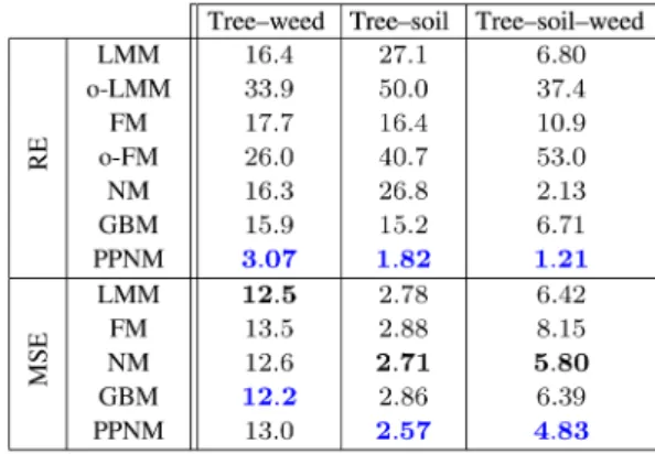
Three types of in situ measured mixed pixels were available to test the different mixing models, i.e., tree–weed, tree–soil, and tree–soil–weed mixtures (see Section III-B). In Table III, the reconstruction error of the mixed signal and the accuracy of the estimated abundances are depicted. From the RE associated with the oracle-LMM, it appears that most nonlinearities occur in the tree-soil mixtures. Once again, PPNM is the mixing model that reconstructs the mixed signatures the best, while FM performed worse than the LMM. For the abundance accuracy, MSE results are less homogeneous than those obtained with the various simulated datasets. Depending on the type of the mixture, GBM or PPNM are the best unmixing model, while FM gives the lowest abundance estimation accuracies.

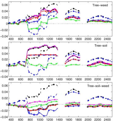
The RDs obtained on the in situ measurements are depicted in Fig. 9. Similarly to the previous analyzed dataset, most of the nonlinear effects seem to occur in the 700–1400 nm spectral range, while being very small in the visible range. From these plots, most of the mixing model appear not sufficiently accurate to capture the nonlinearities in the observed mixtures, except the PPNM.

V. DISCUSSION

The various datasets used during the experiments enable the assessment of the performance of different unmixing models, and the evaluation of the relevance of using nonlinear mixing models to properly describe mixtures observed in vegetated areas. As the exact per-pixel endmembers are known, the effects

of endmember spectral variability can be strongly reduced. Consequently, the simulated or measured mixed pixels can be fully characterized by the abundances, and the influence of the nonlinear mixing effects on the unmixing accuracy could be evaluated. To qualitatively and quantitatively evaluate the mixing models and corresponding unmixing algorithms, general

TABLE II

THREE-ENDMEMBERFORESTSYNTHETICDATASET

Abundance MSE ( ) and RE ( ) for various linear/nonlinear mixing models.

Fig. 8. Three-endmember forest synthetic dataset. Reconstruction difference as a function of wavelength for various linear/nonlinear mixing models: LMM (black), oracle-LMM (black, dashed line), FM (blue), oracle-FM (blue, dashed line), NM (magenta), GBM (red), and PPNM (green).

TABLE III

TWO-ANDTHREE-ENDMEMBERINSITUMEASUREMENTS

Abundance MSE ( ) and RE ( ) for various linear/ nonlinear mixing models.

trends emerge from the results presented in Section IV. These findings are reported in what follows.

A. Quantifying the Amount of Nonlinearity With o-LMM Since the endmember signatures as well as the abundance coefficients are perfectly known for each pixel of the considered scenes, the modeling error (i.e., the RE) obtained with the oracle-LMM could be considered as the mis-modeling introduced by nonlinear mixing effects. For all three data sets, a significant RE can be observed with the oracle-LMM, demonstrating the pres-ence of nonlinear mixing effects, as already shown in [20], [25], [26], for example. In particular, the results reported in Table III show that the in situ-measurements are submitted to highly nonlinear effects. Conversely, from Table II, the forest synthetic dataset seems to be less subjected to these nonlinear effects. Overall, from the results reported in the previous section, the mixed pixel signatures seem to be better represented by nonlinear mixing models, and specifically PPNM and NM. However, all nonlinear mixing models cannot be advocated to better describe mixed pixels than LMM, such as the GBM and NM for the simulated orchard data (see Table I), and the FM for the simulated forest data (see Table II) and the in situ orchard data (see Table III). This shows that these nonlinear mixing models do not necessarily better represent the mixed signatures.

B. On the Use of Reconstruction Error to Assess a Mixing Model It is also important to note that a better modeling of the mixed pixels does not necessarily result in a better estimation of the abundances. For instance, PPNM, which has been shown to be the most accurate to model nonlinearly mixed spectral signa-tures, sometimes lead to less accuracy with respect to the abundance estimation when compared to LMM, in particular for the three-endmember mixtures in the simulated orchard data (see Table I) and for the tree-weed mixtures in the in situ data (see Table III). In the results of the simulated forest, the same trend can be observed: in spite of increasing nonlinear mixing effects, the REs remain almost constant for both the PPNM and the NM, while the accuracy of the estimated abundances decreases (see Table II). As a consequence, the modelfitting error, widely used in the remote sensing literature to monitor the performance of the unmixing algorithm, cannot be used as the uniquefigure-of-merit to evaluate the relevance of a given mixing model.

C. Mismodeling With Respect to Wavelength

All nonlinear mixing models considered in Section II and used in the experiments reported in Section IV implicitly assume the same amount of nonlinearity for each wavelength of the spectral domain. Indeed, they are basically defined by cross-products between the endmember spectra, without introducing any weighting functions that would depend on the spectral bands. However, from the RDs depicted in Figs. 7, 8, and 9, it clearly appears that the mis-modeling is drastically subjected to the influence of the wavelength. This corroborates the results of Somers et al. who also noticed similar behavior for the bilinear mixing model [27]. Most of the nonlinear models under test lead to reconstructed mixtures with the same admissible accuracy as the LMM in the visible range (400–700 nm). Conversely, a clear

degradation of the modeling performance can be observed in the 700–1400 nm spectral range for most linear and nonlinear models, except for the PPNM. In particular, the RDs associated with the oracle-LMM demonstrate the important level of non-linearity in the near-infrared region. Thisfinding has been widely observed in the literature [48]–[50].

D. Dealing With the Unmixing Algorithm Intrinsic Limitations For both LMM and FM models, oracle measures of perfor-mance have been computed since these models are fully de-scribed by the a priori known abundance coefficients, explicitly considered as the spatial distributions of the materials over the imaged pixels. However, for the other nonlinear mixing models, unmixing algorithms need to be used to infer all the parameters involved in the model specification (e.g., abundances and non-linearity parameters). Unfortunately, the optimization problems to be solved, formulated in (11) and (12), to recover the abun-dance coefficients are not totally straightforward, mainly due to the constraints and/or the nonlinearity. As a consequence, the reliability of the obtained results, in terms of RE and abundance MSE, should be carefully analyzed, indeed mitigated. More precisely, part of the REs may consist of approximation errors induced by the unmixing algorithms themselves, in particular when these iterative algorithms converge toward a stationary point which is not the global minimizer of the objective function. Consequently, the abundance estimates may be biased since subjected to these approximation errors. As a manifest example, one can consider the fitting performance of the GBM. By definition, this model generalizes both LMM and FM and, thus, should provide at least similar RE to the lowest RE among those obtained with LMM and FM. However, this is not the case for the

Fig. 9. Two- and three-endmember in situ measurements. Reconstruction dif-ference as a function of wavelength for various linear/nonlinear mixing models: LMM (black), oracle LMM (black, dashed line), FM (blue), oracle FM (blue, dashed line), NM (magenta), GBM (red), and PPNM (green).

orchard synthetic dataset, as already highlight in Section IV-A1 (see Table I). This is an archetypal instance of the limitations of the GBM-based unmixing algorithm.

VI. CONCLUSION

This paper attempted to make a first step toward a full quantitative assessment of linear and nonlinear mixing models to properly described mixtures observed in hyperspectral images acquired over vegetated areas. The conducted work exploited two kinds of hyperspectral data, whose main advantages lies in the availability of ground truth, that consists of the actual material signatures (endmember spectra) and their corresponding spatial repartitions in the pixels (abundance coefficients). The first set of hyperspectral data consisted of physically based simulated images, while the second set of hyperspectral data came from real in situ measurements. Various linear and nonlinear mixing models were used to analyze these data. They were evaluated in terms of spectral mis-modeling (i.e., reconstruction error) and abundance estimation accuracy. From the obtained results, it clearly appeared that the polynomial PPNM undeniably provided, by far, the best reconstruction of the mixed pixels. It also persistently led to admissible abundance estimates, regard-less of the considered scene. More generally, depending of the analyzed mixtures, the Nascimento model, the Fan model or the polynomial postnonlinear model provided the most interesting results with respect to the abundance estimates. However, it was worth noting that the results presented in this work needed to be mitigated by the intrinsic limitations of the resorted unmixing algorithms, that could induce estimate biases. Finally, it is important to admit that the results reported in this work are only valid for two- and three-endmember mixtures. Generalizing or extending thesefindings to more complex scenes would require further investigation.

REFERENCES

[1] J. M. Bioucas-Dias et al.,“Hyperspectral unmixing overview: Geometrical, statistical, and sparse regression-based approaches,” IEEE J. Sel. Topics Appl. Earth Observ. Remote Sens., vol. 5, no. 2, pp. 354–379, Apr. 2012. [2] N. Keshava and J. F. Mustard,“Spectral unmixing,” IEEE Signal Process.

Mag., vol. 19, no. 1, pp. 44–57, Jan. 2002.

[3] B. Somers, G. P. Asner, L. Tits, and P. Coppin,“Endmember variability in spectral mixture analysis: A review,” Remote Sens. Environ., vol. 115, no. 7, pp. 1603–1616, Jul. 2011.

[4] D. C. Heinz and C.-I. Chang,“Fully constrained least-squares linear spectral mixture analysis method for material quantification in hyperspectral imag-ery,” IEEE Trans. Geosci. Remote Sens., vol. 29, no. 3, pp. 529–545, Mar. 2001.

[5] C. Theys, N. Dobigeon, J.-Y. Tourneret, and H. Lantéri,“Linear unmixing of hyperspectral images using a scaled gradient method,” in Proc. IEEE-SP Workshop Stat. Signal Process. (SSP), Cardiff, U.K., Aug. 2009, pp. 729–732.

[6] R. Heylen, D. Burazerovic, and P. Scheunders,“Fully constrained least squares spectral unmixing by simplex projection,” IEEE Trans. Geosci. Remote Sens., vol. 49, no. 11, pp. 4112–4122, Nov. 2011.

[7] N. Dobigeon, J.-Y. Tourneret, and C.-I. Chang,“Semi-supervised linear spectral unmixing using a hierarchical Bayesian model for hyperspectral imagery,” IEEE Trans. Signal Process., vol. 56, no. 7, pp. 2684–2695, Jul. 2008.

[8] O. Eches, N. Dobigeon, C. Mailhes, and J.-Y. Tourneret,“Bayesian esti-mation of linear mixtures using the normal compositional model. Applica-tion to hyperspectral imagery,” IEEE Trans. Image Process., vol. 19, no. 6, pp. 1403–1413, Jun. 2010.

[9] O. Eches, N. Dobigeon, J.-Y. Tourneret, and H. Snoussi, “Variational methods for spectral unmixing of hyperspectral unmixing,” in Proc. IEEE Int. Conf. Acoust. Speech Signal Process. (ICASSP), Prague, Czech Republic, May 2011, pp. 957–960.

[10] N. Dobigeon et al.,“Nonlinear unmixing of hyperspectral images: Models and algorithms,” IEEE Signal Process. Mag., vol. 31, no. 1, pp. 89–94, Jan. 2014.

[11] B. W. Hapke, “Bidirectional reflectance spectroscopy. I. Theory,” J. Geophys. Res., vol. 86, no. B4, pp. 3039–3054, Apr. 1981.

[12] K. J. Guilfoyle, M. L. Althouse, and C.-I. Chang,“A quantitative and comparative analysis of linear and nonlinear spectral mixture models using radial basis function neural networks,” IEEE Trans. Geosci. Remote Sens., vol. 39, no. 8, pp. 2314–2318, Aug. 2001.

[13] J. M. P. Nascimento and J. M. Bioucas-Dias,“Unmixing hyperspectral intimate mixtures,” in Proc. 16th SPIE Image Signal Process. Remote Sens., Oct. 2010, vol. 74830, p. 78300C.

[14] J. Broadwater and A. Banerjee,“A comparison of kernel functions for intimate mixture models,” in Proc. IEEE GRSS Workshop Hyperspectral Image Signal Process.: Evol. Remote Sens. (WHISPERS), Aug. 2009, pp. 1–4.

[15] J. Broadwater and A. Banerjee,“A generalized kernel for areal and intimate mixtures,” in Proc. IEEE GRSS Workshop Hyperspectral Image Signal Process.: Evol. Remote Sens. (WHISPERS), Jun. 2010, pp. 1–4. [16] J. Broadwater and A. Banerjee, “Mapping intimate mixtures using an

adaptive kernel-based technique,” in Proc. IEEE GRSS Workshop Hyper-spectral Image Signal Process.: Evol. Remote Sens. (WHISPERS), Lisbon, Portugal, Jun. 2011, pp. 1–4.

[17] R. Close, P. Gader, A. Zare, J. Wilson, and D. Dranishnikov,“Endmember extraction using the physics-based multi-mixture pixel model,” in Proc. 17th SPIE Imag. Spectrom., Aug. 2012, vol. 8515, pp. 85150L– 85150L-14.

[18] R. Close, P. Gader, J. Wilson, and A. Zare,“Using physics-based macro-scopic and micromacro-scopic mixture models for hyperspectral pixel unmixing,” in Proc. 18th SPIE Algorithms Technol. Multispectral Hyperspectral Ultraspectral Imagery, Apr. 2012, vol. 8390, pp. 83901L–83901L-13. [19] R. Heylen and P. Gader,“Nonlinear spectral unmixing with a linear mixture

of intimate mixtures model,” IEEE Trans. Geosci. Remote Sens., vol. 11, no. 7, pp. 1195–1199, Jul. 2014.

[20] C. C. Borel and S. A. W. Gerstl, “Nonlinear spectral mixing model for vegetative and soil surfaces,” Remote Sens. Environ., vol. 47, no. 3, pp. 403–416, 1994.

[21] T. Ray and B. Murray,“Nonlinear spectral mixing in desert vegetation,” Remote Sens. Environ., vol. 55, no. 1, pp. 59–64, 1996.

[22] L. Zhang, D. Li, Q. Tong, and L. Zheng,“Study of the spectral mixture model of soil and vegetation in Poyang Lake area, China,” Remote Sens. Environ., vol. 19, pp. 2077–2084, 1998.

[23] X. Chen and L. Vierling,“Spectral mixture analyses of hyperspectral data acquired using a tethered balloon,” Remote Sens. Environ., vol. 103, no. 3, pp. 338–350, Aug. 2006.

[24] W. Fan, B. Hu, J. Miller, and M. Li,“Comparative study between a new nonlinear model and common linear model for analysing laboratory simulated-forest hyperspectral data,” Int. J. Remote Sens., vol. 30, no. 11, pp. 2951–2962, Jun. 2009.

[25] B. Somers et al.,“Nonlinear hyperspectral mixture analysis for tree cover estimates in orchards,” Remote Sens. Environ., vol. 113, pp. 1183–1193, Feb. 2009.

[26] L. Tits, W. Delabastita, B. Somers, J. Farifteh, and P. Coppin,“First results of quantifying nonlinear mixing effects in heterogeneous forests: A model-ing approach,” in Proc. IEEE Int. Conf. Geosci. Remote Sens. (IGARSS), 2012, pp. 7185–7188.

[27] B. Somers, L. Tits, and P. Coppin,“Quantifying nonlinear spectral mixing in vegetated areas: Computer simulation model validation andfirst results,” IEEE J. Sel. Topics Appl. Earth Observ. Remote Sens., 2014.

[28] P. Huard and R. Marion,“Study of non-linear mixing in hyperspectral imagery—A first attempt in the laboratory,” in Proc. IEEE GRSS Workshop Hyperspectral Image Signal Process.: Evol. Remote Sens. (WHISPERS), Lisbon, Portugal, Jun. 2011, pp. 1–4.

[29] G. Fontanilles and X. Briottet, “A nonlinear unmixing method in the infrared domain,” Appl. Opt., vol. 50, no. 20, pp. 3666–3677, Jul. 2011.

[30] I. Meganem, P. Déliot, X. Briottet, Y. Deville, and S. Hosseini, “Linear-quadratic mixing model for reflectances in urban environments,” IEEE Trans. Geosci. Remote Sens., vol. 52, no. 1, pp. 544–558, Jan. 2014. [31] Y. Altmann, N. Dobigeon, and J.-Y. Tourneret, “Bilinear models for

nonlinear unmixing of hyperspectral images,” in Proc. IEEE GRSS Workshop Hyperspectral Image Signal Process.: Evol. Remote Sens. (WHISPERS), Lisbon, Portugal, Jun. 2011, pp. 1–4.

[32] Y. Altmann, A. Halimi, N. Dobigeon, and J.-Y. Tourneret,“Supervised nonlinear spectral unmixing using a post-nonlinear mixing model for hyperspectral imagery,” IEEE Trans. Image Process., vol. 21, no. 6, pp. 3017–3025, Jun. 2012.

[33] O. Eches and M. Guillaume,“A bilinear–bilinear non-negative matrix factorization method for hyperspectral unmixing,” IEEE Geosci. Remote Sens. Lett., vol. 11, no. 4, pp. 778–782, Apr. 2014.

[34] J. Stuckens, B. Somers, S. Delalieux, W. W. W. Verstraeten, and P. Coppin, “The impact of common assumptions on canopy radiative transfer simula-tions: A case study in citrus orchards,” J. Quant. Spectrosc. Radiat. Transfer, vol. 110, no. 1–2, pp. 1–21, Jan. 2009.

[35] D. V. der Zande, J. S. W. W. Verstraeten, B. Muys, and P. Coppin, “Assess-ment of light dynamics in broadleaved forest canopies using terrestrial laser scanning,” Remote Sens., vol. 2, no. 6, pp. 1564–1474, 2010.

[36] L. Tits et al.,“Hyperspectral shape-based unmixing to improve intra- and interclass variability for forest and agro-ecosystem monitoring,” ISPRS J. Photogramm. Remote Sens., vol. 74, pp. 163–174, Nov. 2012.

[37] J. M. P. Nascimento and J. M. Bioucas-Dias,“Nonlinear mixture model for hyperspectral unmixing,” in Proc. 15th SPIE Image Signal Process. Remote Sens., 2009, vol. 7477, no. 1, p. 74770I.

[38] A. Halimi, Y. Altmann, N. Dobigeon, and J.-Y. Tourneret,“Nonlinear unmixing of hyperspectral images using a generalized bilinear model,” IEEE Trans. Geosci. Remote Sens., vol. 49, no. 11, pp. 4153–4162, Nov. 2011. [39] A. Taleb and C. Jutten,“Source separation in post-nonlinear mixtures,” IEEE Trans. Signal Process., vol. 47, no. 10, pp. 2807–2820, Oct. 1999. [40] Y. Altmann, N. Dobigeon, and J.-Y. Tourneret,“Nonlinearity detection in hyperspectral images using a polynomial post-nonlinear mixing model,” IEEE Trans. Image Process., vol. 22, no. 4, pp. 1267–1276, Apr. 2013. [41] A. Halimi, Y. Altmann, N. Dobigeon, and J.-Y. Tourneret,“Unmixing

hyperspectral images using the generalized bilinear model,” in Proc. IEEE Int. Conf. Geosci. Remote Sens. (IGARSS), Vancouver, Canada, Jul. 2011, pp. 1886–1889.

[42] D. Van der Zande,“Mathematical modeling of 3D canopy structure in forest stands using ground-based Lidar,” Ph.D. dissertation, Katholieke Univer-siteit Leuven, Leuven, Belgium, 2008.

[43] M. Pharr and G. Humphreys, Physically Based Rendering: From Theory to Implementation. San Mateo, CA, USA: Morgan Kaufmann, 2004. [44] J. Weber and J. Penn, “Creation and rendering of realistic trees,”

in Proc. SIGGRAPH Annu. Conf. Comput. Graph. Interact. Tech., 1995, pp. 119–128.

[45] FAO,“FAO world reference base for soil resources,” Food and Agriculture Organisation of the United Nations, Rome, Italy, World Soil Resource Rep. 84, 1998.

[46] B. Somers, V. Gysels, W. Verstraeten, S. Delalieux, and P. Coppin,“Model-ling moisture-induced soil reflectance changes in cultivated sandy soils: A case study in citrus orchards,” Eur. J. Soil Sci., vol. 61, no. 6, pp. 1091–1105, 2010.

[47] B. Hosgood et al.,“Leaf optical properties experiment 93 (LOPEX93),” Joint Research Centre/Inst. Remote Sens. Appl. Unit Advanced Techn., Ispra, Italy, Rep. EUR 16095 EN, 1995.

[48] A. R. Huete, R. D. Jackson, and D. F. Post,“Spectral response of a plant canopy with different soil backgrounds,” Remote Sens. Environ., vol. 17, no. 1, pp. 37–53, Feb. 1985.

[49] N. S. Goel,“Models of vegetation canopy reflectance and their use in estimation of biophysical parameters from reflectance data,” Remote Sens. Rev., vol. 4, no. 1, pp. 1–212, 1988.

[50] S. Jacquemoud, C. Bacour, H. Poilvé, and J.-P. Frangi,“Comparisons of four radiative transfer models to simulate plant canopies reflectance: Direct and inverse mode,” Remote Sens.Environ., vol. 74, no.3,pp. 471–481, Dec.2000. Nicolas Dobigeon (S’05–M’08–SM’13) was born in Angoulême, France, in 1981. He received the Engi-neering degree in electrical engiEngi-neering from École nationale supérieure d’électronique, d’électrotechni-que, d’informatique, d’hydraulique et des télécommu-nications (ENSEEIHT), University of Toulouse, Toulouse, France, in 2004, the M.Sc. degree in signal processing from the National Polytechnic Institute (INP) of Toulouse, Toulouse, France, in 2004, and the Ph.D. degree and Habilitation Diriger des Re-cherches in signal processing from INP Toulouse in 2007 and 2012, respectively.

From 2007 to 2008, he was a Postdoctoral Research Associate with the Department of Electrical Engineering and Computer Science, University of Michigan, Ann Arbor, MI, USA. Since 2008, he has been with National Polytechnic Institute (INP) of Toulouse, University of Toulouse, where he is currently an Associate Professor. He conducts his research within the Signal and

Communications Group, IRIT Laboratory, and is also an Affiliated Faculty Member of the TeSA Laboratory. His research interests include statistical signal and image processing, with a particular interest in Bayesian inverse problems with applications to remote sensing, biomedical imaging, and genomics.

Laurent Tits received the M.Sc. and Ph.D. degrees in bioscience engineering (land and forest management) from the Katholieke Universiteit (KU) Leuven, Leuven, Belgium, in 2009 and 2013, respectively.

Since 2010, he has been a Research Assistant with the Geomatics Engineering Group, Department of Biosystems, KU Leuven. His research interests in-clude hyperspectral as well as thermal remote sensing in vegetative systems, with a specific focus on spectral and thermal mixture analysis.

Ben Somers was born in Leuven, Belgium, on Sep-tember 13, 1982. He received the M.Sc. and Ph.D. degrees in bioscience engineering (land and forest management) from the Katholieke Universiteit Leuven (KU Leuven), Leuven, Belgium, in 2005 and 2009, respectively.

In 2010, he was a Research Associate with the Geomatics Engineering Group, KU Leuven. Between 2011 and 2013, he was a Researcher with the Remote Sensing Division, Flemish Institute for Technological Research (VITO), Antwerp, Belgium.

In October 2013, he started as an Assistant Professor (tenure track position) with the Division Forest, Nature and Landscape, Department of Earth and Environmental Sciences, KU Leuven. He is experienced in the design and integration of the state-of-the-art remote sensing techniques to study the impact of disturbance processes (nutrient deficiencies, pests and diseases, invasive exotic species, and climate change) on the functioning of terrestrial ecosystems. His research interests include fostering the use and application of remote sensing in support of sustainable management of seminatural and urban environments.

Yoann Altmann (S’10–M’14) was born in Toulouse, France, in 1987. He received the Engineering degree in electrical engineering from École nationale supér-ieure d’électronique, d’électrotechnique, d’informa-tique, d’hydraulique et des télécommunications, University of Toulouse, Toulouse, France, in 2010, the M.Sc. degree in signal processing from the National Polytechnic Institute of Toulouse (INP Toulouse), Toulouse, France, in 2010, and the Ph.D. degree in signal processing from INP Toulouse, in 2013.

Since 2014, he has been with the Heriot-Watt University, Edinburgh, U.K. as a Postdoctoral Researcher. He conducts his research within the Institute of Sensors, Signals and Systems, School of Engineering and Physical Sciences. His research interests include statistical signal and image processing, with a particular interest in Bayesian inverse problems with applica-tions to remote sensing and biomedical imaging.

Pol Coppin received the M.Sc. degree from Univer-siteit Gent, Gent, Belgium, in 1977, and the Ph.D. degree from University of Minnesota, Minneapolis, MN, USA, in 1991.

Currently, he is a Chair Professor in Geomatics Engineering with the Katholieke Universiteit (KU) Leuven, Leuven, Belgium. His research team forms part of the Division Measure, Model and Manage Bio-Responses within the Bio-Systems Department and focuses on the monitoring and modeling of plant production systems. He is a project leader on the Flemish side for the joint Flemish-South African IS-HS program and responsible for the hyperspectral sensor, the electronic bundle-steered antenna, the transpon-der technology for on-board communication with ground sensor suites, and the integrated monitoring and modeling of plant systems. His career spans 12 years of professional experience (1977–1988 and many short-term missions afterward) in tropical and subtropical natural resources assessment and monitoring, followed by an academic career at the University of Minnesota and Purdue University, West Lafayette, IN, USA (1988–1995), and at the KU Leuven (1995–present).