Sounding out ecoacoustic metrics: Avian species richness is predicted by acoustic indices in temperate but not tropical habitats

(1)

Any correspondence concerning this service should be sent

to the repository administrator:

tech-oatao@listes-diff.inp-toulouse.fr

This is an author’s version published in:

http://oatao.univ-toulouse.fr/22642

To cite this version:

Eldridge, Alice and Guyot, Patrice and

Moscoso, Paola and Johnston, Alison and Eyre-Walker, Ying and

Peck, Mika Sounding out ecoacoustic metrics: Avian species

richness is predicted by acoustic indices in temperate but not

tropical habitats. (2018) Ecological Indicators, 95 (1). 939-952.

ISSN 1470-160X

Official URL

DOI :

https://doi.org/10.1016/j.ecolind.2018.06.012

Open Archive Toulouse Archive Ouverte

OATAO is an open access repository that collects the work of Toulouse

researchers and makes it freely available over the web where possible

(2)

Sounding

out ecoacoustic metrics: Avian species richness is predicted by

acoustic

indices in temperate but not tropical habitats

Alice

Eldridge

a,b,⁎

,

Patrice Guyot

c

,

Paola Moscoso

b

,

Alison Johnston

d,e

,

Ying Eyre-Walker

b

,

Mika Peck

b

a_{Department of Music, School of Media, Film and Music, University of Sussex, UK} b_{Evolution Behaviour & Environment, School of Life Sciences, University of Sussex, UK} c_{Institut de Recherche en Informatique de Toulouse (IRIT), Université Toulouse, France} d_{Conservation Science Group, Department of Zoology, University of Cambridge, UK} e_{Cornell Lab of Ornithology, Cornell University, Ithaca, NY 14850, USA}

Keywords: Biodiversity monitoring Remote sensing Ecoacoustics Acoustic indices Species richness A B S T R A C T

Affordable, autonomous recording devices facilitate large scale acoustic monitoring and Rapid Acoustic Survey is emerging as a cost-effective approach to ecological monitoring; the success of the approach rests on the de-velopment of computational methods by which biodiversity metrics can be automatically derived from remotely collected audio data. Dozens of indices have been proposed to date, but systematic validation against classical, in situ diversity measures are lacking. This study conducted the most comprehensive comparative evaluation to date of the relationship between avian species diversity and a suite of acoustic indices. Acoustic surveys were carried out across habitat gradients in temperate and tropical biomes. Baseline avian species richness and subjective multi-taxa biophonic density estimates were established through aural counting by expert ornithol-ogists. 26 acoustic indices were calculated and compared to observed variations in species diversity. Five acoustic diversity indices (Bioacoustic Index, Acoustic Diversity Index, Acoustic Evenness Index, Acoustic Entropy, and the Normalised Difference Sound Index) were assessed as well as three simple acoustic descriptors (Root-mean-square, Spectral centroid and Zero-crossing rate). Highly significant correlations, of up to 65%, between acoustic indices and avian species richness were observed across temperate habitats, supporting the use of automated acoustic indices in biodiversity monitoring where a single vocal taxon dominates. Significant, weaker correlations were observed in neotropical habitats which host multiple non-avian vocalizing species. Multivariate classification analyses demonstrated that each habitat has a very distinct soundscape and that AIs track observed differences in habitat-dependent community composition. Multivariate analyses of the relative predictive power of AIs show that compound indices are more powerful predictors of avian species richness than any single index and simple descriptors are significant contributors to avian diversity prediction in multi-taxa tropical environments. Our results support the use of community level acoustic indices as a proxy for species richness and point to the potential for tracking subtler habitat-dependent changes in community composition. Recommendations for the design of compound indices for multi-taxa community composition appraisal are put forward, with consideration for the requirements of next generation, low power remote monitoring networks.

1. Introduction

Numerous global initiatives aim to conserve biodiversity (e.g. United Nations Sustainable Development Goals, Convention on Biological Diversity AICHI biodiversity targets, REDD++), but action can only be eﬀectively taken if biodiversity can be measured and its rate of change quantiﬁed (Buckland et al., 2005). Coupled with rapid changes in landscape use (Betts et al., 2017; Newbold et al., 2015) the

impact of climate change (Stocker et al., 2013) and growing fragmen-tation of natural landscapes globally (Crooks et al., 2017), the devel-opment of cost eﬀective methods for biodiversity monitoring at scale is an urgent global imperative (Newbold et al., 2015).

1.1. Ecoacoustics and rapid acoustic survey

Operating within the conceptual and methodological framework of

⁎_{Corresponding author at: Arts B B156, University of Sussex, Falmer, Brighton, East Sussex BN1 9QN, UK.}

E-mail address:alicee@sussex.ac.uk(A. Eldridge).

(3)

wider acoustic environment – or soundscape (Pijanowski et al., 2011). Whilst there is an established tradition of aural survey of individual species (as in point counts), ecoacoustics aims to develop the study and theory of population, community or landscape level bioacoustics. The prevailing predicate of RAS is that higher species richness in a given community will produce a greater ‘range’ of signals, resulting in a greater acoustic diversity (Gasc et al., 2013; Sueur et al., 2014; Sueur et al., 2008).

Based on this premise, indices to measure within-group (alpha) and between-group (beta) indices have been proposed (Sueur et al., 2014). The current concern is validation against traditional metrics derived from species counts, therefore we focus on alpha indices. These are designed to estimate amplitude (intensity), evenness (relative abun-dance), richness (number of entities) and heterogeneity of the acoustic community. A suite of indices was made available via R packages see-wave [1] (Sueur et al., 2008) [1] and soundecology [2] ( Villanueva-Rivera et al., 2011) and has been rapidly taken up in ecological research – the libraries exceeding 61,000 downloads since 2012. However, ex-perimental investigation of the relationship between these, and other acoustics metrics, with traditional, in situ biodiversity measures reveals mixed, and at times contradictory results (Boelman et al., 2007; Fuller et al., 2015; Mammides et al., 2017). Furthermore, simulation studies (Gasc et al., 2013) demonstrate that acoustic diversity can be influ-enced by sources of acoustic heterogeneity other than species richness, including variation in distance of animals to the sensors, and inter- and intra-specific differences in calling patterns and characteristics (e.g. duration, intensity, complexity of song, mimicry). The premise that biodiversity can be inferred from acoustic diversity is percipient but not fully substantiated: before these proposed indices can be confidently adopted for monitoring purposes, it is critical to understand i) how well AIs capture ecologically meaningful changes in community composition and ii) how robust they are to diverse ecological, environmental, and acoustic conditions. To this end, this study carried out the largest sys-tematic, comparative study of the relationship between acoustic indices and observed avian diversity to date.

1.3. Acoustic indices

1.3.1. Ecologically inspired diversity indices

Early research led to the development of indices derived from landscape metrics (Turner, 1989) to measure changes at the level of soundscape (Gage et al., 2001; Napoletano, 2004). The Normalised Difference Sound Index (NDSI) (Kasten et al., 2012) seeks to describe the level of anthropogenic disturbance by calculating the ratio of mid-fre-quency biophony to lower fremid-fre-quency technophony in field recordings, the values for each being computed from an estimate of power density spectrum (Welch, 1967). In long term studies, the NDSI has been shown to reflect assumed seasonal and diurnal variation across landscapes (Kasten et al., 2012). It has subsequently been shown to be sensitive to biophony and anthrophony levels in urban areas (Fairbrass et al., 2017) and to be an indicator of anthropogenic presence in the Brazilian Cer-rado (Alquezar and Machado, 2015). NDSI has also been evaluated as a proxy for species diversity with mixed results: significant relationships with bird species richness have reported across mixed habitats in China (Mammides et al., 2017); in Brazilian savanna habitats no relationships were observed (Alquezar and Machado, 2015).

Based on the foundational premise that biodiversity can be inferred from acoustic diversity, several indices draw an analogy between spe-cies distribution and distribution of energy in a spectrum, where each frequency band is seen to represent a speciﬁc ‘species’. The entropy indices Hf and Ht (Sueur et al., 2008) are calculated as the Shannon entropy of a probability mass function (PMF) and designed to increase Fig. 1. The acoustic environment, or soundscape, is comprised of sounds made

by noisy biotic and abiotic processes, including biological organisms (biophony), geological forces (geophony) and humans and machines (anthro-phony/technophony). Acoustic indices provide terse numerical descriptions of the overall soundscape. The use of acoustic indices as a proxy for biodiversity is predicated on the assumption ﬁrstly that the acoustic community of vocalising creatures is representative of the wider ecological community and secondly that the facets of soundscape dynamics captured by acoustic indices are ecologi-cally-meaningful. The current working hypothesis is that higher species rich-ness will generate greater acoustic diversity; a suite of indices aimed at cap-turing spread and evenness of acoustic energy have been proposed but have yet to be conclusively validated against traditional, in situ biodiversity metrics.

[1]_{https://cran.r-project.org/web/packages/seewave/}_. [2]

https://cran.r-project.org/web/packages/soundecology/. ecoacoustics (Sueur and Farina, 2015) Rapid Acoustic Survey (RAS)

(Sueur et al., 2008) has been proposed as a non-invasive, cost-effective approach to Rapid Biodiversity Assessment (Mittermeier and Forsyth, 1993) and is gaining interest from researchers, decision-makers and conservation managers alike. Whereas bioacoustics infers behavioural information from intra- and interspecific signals, ecoacoustics in-vestigates the ecological role of sound at higher organisational units – from population and community up to landscape scales. Sound is un-derstood as a core ecological component (resource) and therefore in-dicator of ecological status (source of information). Rather than at-tempting to identify specific species calls, RAS aims to infer biodiversity at these higher levels of organization, through the collection and computational analysis of large scale acoustic recordings. RAS is a highly attractive solution for large scale monitoring, because it is non-invasive, obviates the need for expert aural identification of individual recordings, scales cost-effectively and is potentially sensitive to mul-tiple taxa. This approach has potential to dramatically improve remote biodiversity monitoring, enabling data collection and analysis over previously inaccessible spatio-temporal scales, including in remote, hostile, delicate regions in both terrestrial and marine environments. The success of the approach rests on the development and validation of computational metrics, or acoustic indices, which demonstrably predict some facet of biodiversity.

1.2. Acoustic indices for biodiversity monitoring

Whereas classical biodiversity indices are designed to enumerate some facet of biotic community diversity at a particular time and place – richness, evenness, regularity, divergence or rarity in species abun-dance, traits or phylogeny (Magurran, 2013; Magurran and McGill, 2011; Pavoine and Bonsall, 2011) – acoustic indices are designed to capture the distribution of acoustic energy across time and/or frequency in a digital audio file of fixed length. As illustrated in Fig. 1, the use of acoustic indices (AIs) as ecological indicators is predicated firstly on the assumption that the acoustic community (Gasc et al., 2013) is re-presentative of the wider ecological community at the place and time of interest; and secondly that computationally measurable changes in the acoustic environment are ecologically relevant. An effective index will reflect ecologically meaningful changes in the acoustic community, whilst being insensitive to potentially confounding variations in the

(4)

time or frequency) domain are necessary in order to rigorously in-vestigate the dynamic composition of acoustic environments. However, in applied monitoring tasks, we are primarily concerned with cost-ef-fectiveness, validity and reliability across ecological conditions. Looking toward future application of in situ analyses, eﬃciency in computational and logistical terms become important factors; with this in mind it becomes pertinent to consider how new ecological acoustic metrics might take inspiration from machine listening applications in other domains.

1.3.3. Simple acoustic descriptors

As micro-processors become smaller, cheaper and more powerful and techniques for data transfer in low-power networks of embedded systems advance, the possibility for in situ computation becomes very real. This could be very useful for long-term applications where col-lection and storage of raw audio data is unreasonable, such as phe-nology monitoring. Under this emerging protocol, computational effi-ciency of AIs becomes more important as lower computational cost equates to lower energetic cost, or energy complexity (Zotos et al., 2005); reducing energetic cost could afford the development of net-works of solar-powered devices, further increasing feasibility of long term monitoring in remote locations. Machine learning methods are too computationally intensive for these situations and we look instead to parsimonious solutions which are computationally and energetically cheap. A large body of research in machine listening in music, speech and non-ecological environmental sound analyses demonstrates the power of simple acoustic descriptors in automated classification tasks. Here we select three to test alongside the suite of existing ecoacoustic diversity indices. These provide information about amplitude, spectral, and temporal characteristics: Root-mean-square (RMS) of the raw audio signal, spectral centroid (SC) and zero-crossing rate (ZCR), described below.

The root-mean-square (RMS) of the raw audio signal gives a simple description of signal amplitude; RMS has been demonstrated to track ecologically-relevant temporal and spatial dynamics in forest canopy (Rodriguez et al., 2014), and shown to be strongly positively correlated with percentage of living coral cover in tropical reefs (Bertucci et al., 2016), but has not been investigated in recent terrestrial correlation studies. Mean values are expected to increase with acoustic activity, variance may more accurately track avian vocalisations under the same logic as ACI. Spectral centroid provides a measure of the spectral centre of mass; it is widely used in machine listening tasks where is it re-cognized to have a robust connection with subjective measures of brightness. This and related spectral indices have been shown to be effective in automated recognition of environmental sounds in urban environments (Devos, 2016). Zero-crossing rate (ZCR) is one of the simplest time-domain features, which in essence reflects the rate at which sound waves impact on the microphone. ZCR provides a measure of noisiness (being high for noisy, low for tonal sounds) and is widely used in speech recognition and music information retrieval, for example as a key feature in the classification of percussive sounds (Gouyon et al., 2002). SC and ZCR have been demonstrated to be useful descriptors in classification of habitat type (Bormpoudakis et al., 2013), but have yet to be evaluated as proxies for species diversity. We expect a negative association with avian activity for both: relative to the quiet broad-band noise of inactivity, avian vocalisations are predicted to be of lower frequency and more harmonic, resulting in a lower spectral centroid and zero-crossing rate. We might also expect the variance of each to positively track activity as the onsets of avian calls will cause rapid changes in values.

1.4. Validation requirements

To assess the potential for these indices as ecological indices, ex-plicit comparison with established biodiversity metrics is a critical ﬁrst step (Gasc et al., 2017). In order to validate the near-term application of with species diversity. For Hf the PMF is derived from the mean

spec-trum, for Ht from the amplitude envelope. Their product is H. Early studies reported higher values for intact over degraded tropical forests (Sueur et al., 2008), but subsequent testing in a temperate woodland reported contradictory results, attributed to background technophonies (Depraetere et al., 2012). H has since been reported to show positive, moderate correlations with avian species richness across multiple ha-bitats in China (Mammides et al., 2017) and a variant of Ht (Acoustic Richness) was shown to be positively associated with observed species richness (Depraetere et al., 2012). These entropy and evenness mea-sures encapsulate the foundational assumption of RAS, but are not in-tuitive to interpret.

The Acoustic Evenness and Acoustic Diversity Indices (AEI, ADI) are motivated by a similar analogy between species distribution and dis-tribution of sound energy. Both are calculated by first dividing the spectrogram into N bins across a given range (typically 0–10 kHz) and taking the proportion of signal in each bin above a set threshold. ADI is the result of the Shannon Entropy (Jost, 2006) applied to the resultant vector; AEI is the Gini coefficient (Gini, 1971), providing a measure of evenness. These were originally developed to assess habitats along a gradient of degradation under the assumption that ADI and AEI would be respectively positively and negatively associated with habitat status as the distribution of sounds became more even with increasing di-versity (Villanueva-Rivera et al., 2011): ADI was shown to increase from agricultural to forested sites; AEI was shown to decrease over the same gradient, as expected. Negative, if weak, associations between AEI and biocondition (Eyre et al., 2015) have subsequently been corrobo-rated (Fuller et al., 2015) and a significant positive association between ADI and avian species richness has been reported in the savannas of central Brazil (Alquezar and Machado, 2015).

Rather than applying extant ecological metrics to acoustic data, other ecoacoustic indices have been designed more intuitively; the Bioacoustic Index (BI) was designed to capture overall sound pressure levels across the range of frequencies produced by avifauna (Boelman et al., 2007). BI was originally reported to correlate strongly with changes in avian abundance in Hawaiian forests (Boelman et al., 2007), but subsequent assessments have been mixed, showing significant as-sociation with avian species richness (Fuller et al., 2015) and both positive and negative weaker correlations (Mammides et al., 2017) in areas with multiple vocalizing taxa. Despite an initially strong de-monstration of efficacy, and conceptual and computational simplicity, this index has been excluded from many recent analyses (Harris et al., 2016). In response to observations that many of these indices are over-sensitive to ‘background’ noise, the Acoustic Complexity Index (ACI) was developed (Pieretti et al., 2011). ACI reports short-time averaged changes in energy across frequency bins, with the aim of capturing transient biophonic sounds, whilst being insensitive to more continuous technophonies such as airplanes and other engines. ACI has been re-ported to correlate significantly with the number of avian vocalisations in an Italian national park (Pieretti et al., 2011), with observed species evenness and diversity in temperate reefs (Harris et al., 2016) and to be positively related to observed changes in migratory avian species numbers in a multi-year Alaskan study (Buxton et al., 2016). A recent urban study reports correlations between ACI and biotic activity and diversity, as well as anthrophonic signals (Fairbrass et al., 2017), as expected, given the full range analyses carried out.

1.3.2. Machine learning derived indices

In contrast to these relatively simple indices, more sophisticated supervised and unsupervised machine learning methods have also been proposed (Phillips et al., 2018; Towsey et al., 2014). In a single site comparative study (Towsey et al., 2014) describe a spectral clustering algorithm which is shown to be the strongest indicator of species number, outperforming many of the indices described above. In pre-vious work (Eldridge et al., 2016; Guyot et al., 2016) we have suggested that more complex analyses that operate in time-frequency (rather than

(5)

of multi-habitat studies. Similarly, more recent research evaluating indices directly against observed species diversity in terrestrial (Alquezar and Machado, 2015; Mammides et al., 2017), aquatic (Harris et al., 2016) and urban (Fairbrass et al., 2017) contexts conclude that whilst the approach holds promise, no single index can yet be reliably adopted as a proxy for biodiversity. These studies have tended to focus on small sets of indices and been carried out in a constrained set of biomes: the requisite comparative correlation study across habitats which support diverse acoustic communities and acoustic density gra-dients has yet to be performed.

Here we carry out a systematic, comparative analysis of AIs across a wide range of ecological conditions in both temperate and neotropical ecozones. The principle aim was to evaluate the response of a range of acoustic indices to observed changes in avian diversity, across a range of ecological conditions, in order to both evaluate current indices as ecological indicators and to inform the design of future indices suitable for low power devices. To this end, the suite of diversity indices pro-posed inSueur et al. (2014)were compared with parsimonious acoustic descriptors commonly used in other machine listening tasks.

Two principle questions were addressed:

i) Do existing AIs track observed diﬀerences in avian diversity? ii) Are compound indices more powerful predictors of avian species

diversity than any single index? Two meta questions applied to both:

- How does the presence of other vocalising species impact these re-lationships?

- How do simple acoustic descriptors compare to bespoke ecoacoustic diversity indices?

2. Methods 2.1. Study sites

Acoustic surveys were carried out along a gradient of habitat de-gradation (1 forested, 2 regenerating forest and 3 agricultural land) in South East (SE) England and North Western (NW) Ecuador. The six sites (UK1, UK2, UK3, EC1, EC2, EC3) were sampled consecutively from May 6th to Aug 25th 2015.

All UK sites were in the county of Sussex, in SE England, an area of weald clays (Fig. 2, left) and included ancient woodland (UK1), re-generating farmland with patches of woodland (UK2) and a downland barley farm (UK3). Ecuadorian sites (Fig. 2, right) were situated in the NW of the country and included primary forest (EC1), secondary forest (EC2) and palm oil plantation (EC3). SeeSupplementary materialA for details.

Fig. 2. Locations of sampling sites in the UK (left) and Ecuador (right): Forest Site, UK1 (N 50° 55′ 16.763″ E 0°5′ 23.071″); Secondary Forest, UK2 (N 50° 58′ 8.548″ W 0° 22′ 40.646″); Agricultural site, UK3 (N 50° 58′ 8.548″ W 0° 22′ 40.646″. Primary Forest, EC1, (N 0° 32′ 17.628″ W 79° 8′ 34.728″); Secondary Forest, EC2 (N 0° 7′ 12.320″ W 9° 16′ 37.103″) Agricultural, EC3 (N 0° 7′ 48.864″ W 79° 12′ 59.543″ existing AIs in monitoring tasks and to inform the development of more

eﬀective indices for the future, we suggest at least three experimental conditions are necessary: i) variation in ecological conditions ii) spatial and or temporal replication iii) comparisons between individual indices as well as compound metrics.

Any ecological indicator must be demonstrably robust to variation in ecological conditions. For acoustic indices, this includes variations in habitat structure, which affects signal propagation, as well as hetero-geneity of acoustic environment due to non-biotic sound sources (an-throphony and geophony) and crucially, the diversity and density of vocalising taxa. The impact of environmental dissimilarity on correla-tions between the diversity indices and avian species richness was re-cently shown to be non-significant (Mammides et al., 2017). Re-sponding to recognition that existing indices are known to be sensitive to ‘background’ noise (Depraetere et al., 2012), Fairbrass et al. (2017) compared the response of four AIs (ACI, BI, ADI, and NDSI) in urban environments and demonstrated that all were sensitive to anthrophony, questioning their application in urban areas (Fairbrass et al., 2017). Although understanding the performance of AIs in environments with varying diversity and density of vocalising taxa is fundamental, few studies have explicitly addressed this. Recent correlation studies have focused on avian species richness alone, without tracking other taxa, despite being carried out in tropical environments characterised by high insect and amphibian activity (Alquezar and Machado, 2015; Fuller et al., 2015; Mammides et al., 2017). This makes interpretation of results difficult. Where other multiple taxa have been considered, the focus has generally been on identifying and removing specific cate-gories of sound, such as cicada choruses (Towsey et al., 2014). Corre-lation studies to date have also been predominantly carried out at the peak activity of dawn chorus (Boelman et al., 2007; Mammides et al., 2017), which is a demonstrably efficient sampling strategy (Wimmer et al., 2013), but precludes investigation of the response of AIs to variation in vocalization density.

Carrying out spatially and/or temporally replicated surveys is im-portant because existing indices are known to be sensitive to local differences in vocalisation patterns (Gasc et al., 2013; Sueur et al., 2014). If there are strong community level differences in acoustic communities we might expect that as survey size increases, the effect of local variation in individuals, species, vegetation structure or other acoustic events will decrease, cancelling out as noise.

Finally, comparative studies are vital because no single index is likely to give complete and reliable information about the diversity and state of any given ecosystem – just as no single biodiversity index will re-liably estimate all levels of local or regional biodiversity (Sueur et al., 2014). Towsey et al. (2014) provided a thorough investigation of multiple indices relative to a comprehensive avifauna census dataset and showed that a linear combination can be more powerful than any single index, however they also note that their results are over-ﬁtted, and do not generalise to other habitats, further stressing the importance

(6)

logged separately and combined (averaged) to provide an indication of the contribution of non-avian taxa to the acoustic community. Ordinal descriptors of rain, wind, motor noise, human and ‘other’ sounds were also recorded and assigned a value in the range 0–4 to describe the level of other soundscape components. SeeSupplementary material B for instructions given to ornithologists.

2.4. Filtering and screening

All recordings were pre-processed with a high pass filter (HPF) with a cut off of 300 Hz (12 dB). Pre-processing recordings with a HPF at 1 kHz is common as low frequency energy is often considered difficult to interpret, being affected by atmospheric noise (Napoletano, 2004); we reduced the threshold in order to minimise loss of relevant low frequency biophony of Ecuadorian species. The HPF also rectified a variable DC offset inherent in the SM3 machines. The main analyses focused on the files which had been listened to by the ornithologists (the labelled data set). Of these, files labelled as distorted by wind, rain or electrical fault (assigned values of 4) were excluded leaving 1976 and 1201 samples for UK and Ecuador respectively.

2.5. Acoustic indices

Seven of the core indices included in R libraries Seewave and Soundecology were investigated from ﬁve categories (ACI, ADI & AEI, BI, Hf & Ht, NDSI) along with three simple low level acoustic de-scriptors (RMS, SC, ZCR). Acoustic Richness was not used as it is a ranked index, obviating inclusion in correlation analyses where each record is treated as a statistical individual. Indices were calculated across 0–24 kHz for each 1 min ﬁle otherwise stated.

1.Acoustic Complexity Index (ACI) (Pieretti et al., 2011) is calcu-lated as the average absolute fractional change in spectral amplitude (across 0.3–24 kHz) for each frequency bin in consecutive spec-trums. The main ACI value is the average value over 1 min using default parameters (J = 5 bins per second).

2.Acoustic Diversity Index (ADI) and Acoustic Evenness Index (AEI) (Villanueva-Rivera et al., 2011) are calculated by ﬁrst dividing a spectrogram into 10 bins (min–max 0–10 kHz), normalizing by the maximum, and taking the proportion of the signals in each bin above a threshold (-50 dBFS). AD is the result of the Shannon En-tropy of the resultant vector; AE is the Gini coeﬃcient, providing a measure of evenness.

3.Bio-acoustic Index (BI) (Boelman et al., 2007) is calculated as the area under the mean spectrum (in dB) minus the minimum dB value of this mean spectrum across the range 2–8 kHz.

4.Spectral and Temporal Entropy (Hf and Ht) (Sueur et al., 2008) are calculated as the Shannon entropy of a probability mass function (PMF). For Hf the PMF is derived from the mean spectrum, for Ht from the amplitude envelope.

5.Normalised Diﬀerence Sound Index (NDSI) (Kasten et al., 2012) is the ratio (biophony − anthrophony)/(biophony + anthrophony). The values for each are computed from an estimated power spectral density using Welch's method (win = 1024) where anthrophony is the sum of energy in the range 1–2 kHz and biophony across 2–11 kHz.

6.Root-Mean-Square (RMS) is calculated by taking the root of the mean of the square of samples in each frame (N = 512).

7.Spectral Centroid (SC) (Peeters, 2004) is calculated as the weighted mean of the frequencies present in the signal, per frame, determined from an SSFT where the weights are the magnitudes for each bin.

8.Zero-Crossing Rate (ZCR) (Peeters, 2004) is the number of times the time domain signal value crosses the zero axis, divided by the frame size.

2.2. Acoustic survey methods

Ten day acoustic surveys were carried out consecutively at each study site using 15 Wildlife Acoustics Song Meter audio ﬁeld recorders. Sampling points were arranged in a grid at a minimum distance of 200 m to minimise pseudo replication (the sound of most species being attenuated over this distance in all biomes). Altitudinal range of sample points across sites was minimised in order to prevent introduction of extraneous, confounding gradients. UK sites were within an elevational range of 10 m–50 m and Ecuador 130 m–390 m. Recording schedules captured 1 min every 15 min around the clock for 10 days at each site, resulting in 960 stereo recordings at each of 15 sample points for 3 habitat types in 2 diﬀerent climates (86,400 1 min stereo recordings in total). Data across the 15 sample points was pooled; inter-site variation was not explored in the current analyses. In the UK 3½ h of each dawn chorus was sampled starting at 1 h before sunrise. This range was de-termined to capture the onset, progression and peak of the dawn chorus, creating a temporal gradient. The equatorial dawn chorus is more compact and was sampled for 2¼ h starting 15 min before sunrise, capturing a comparable chorus onset and peak.

The Song Meter is a schedulable, oﬀ-line, weatherproof recorder, with two channels of omni-directional microphone (ﬂat frequency re-sponse between 20 Hz and 20 kHz). Seven SM2+ _{and eight SM3 devices}

were deployed. Gains were matched between models (analogue gains at +36 dB on SM2+ _{and +12 dB on SM3 which has inbuilt +12 dB gain)}

and recordings made at resolution of 16 bits with a sampling rate of 48 kHz.

Local weather was recorded for each site using Met Oﬃce data from the nearest station in the UK (max 20 km distance) and a portable weather station located within 1 km of each study site in Ecuador. These data were used to select a subset of 3 consecutive days based on lowest wind speeds and rainfall for each habitat.

2.3. Avian species identiﬁcation and soundscape descriptors

In both ecozones all 15 survey points for each habitat were analysed over the 3 day subset for each of the 3 habitat types in both ecozones, giving a total of 2025 UK files (15 samples for each dawn over 3 days for 15 points for 3 sites) and 1350 Ecuadorian files (10 samples at dawn over 3 days for 15 sample points across 3 habitats). Stereo files were split and the channel with least distortion (due to wind, rain or faults) for each habitat type was preserved.

These data subsets (2025 mono files for the UK and 1350 for Ecuador) were labelled with avian species and soundscape descriptors by ornithologists. Files were anonymised, randomised and presented to ornithologists expert to each ecozone (Joseph Cooper in the UK and Manuel Sanchez in Ecuador) who established vocalising species rich-ness (N0) values by identifying each avian species heard in each minute file; an abundance proxy (NN) was achieved by recording the maximum number of simultaneous vocalisations heard for each species. Their labels were verified by a second expert for each ecozone (Penny Green in the UK and Jorge Noe Morales in Ecuador) who each listened to a randomized 10% of the labelled files for their respective ecozone. Pearson’s correlation coefficient on species richness between these verified subsets showed acceptable agreement (R = 0.85 for UK and 0.77 for Ecuador). Species ID from recording has recently been shown to be more powerful than traditional in situ point count, despite the loss in visual registers, and adopted here to ensure compatibility with acoustic computational methods (Darras et al., 2017).

In order to establish the presence of other vocalizing species and enable comparison of indices with overall activity of the acoustic community, a subjective measure of biophonic density (BD) was recorded in the range 0–3, describing the percentage of time vocalisations of speciﬁc taxa occurred across each 1 min sample (0–25%, 25–50%, 50–75% and 75–100%). In the UK biophonic density included only avian calls; in Ecuador avian, amphibian and insect vocalisations were

(7)

was built for each ecozone using all 26 AIs as predictors and species richness as the response. Nine AIs were used at each split with a minimum terminal node size of 10. AIs and species richness values were first standardised (μ = 0, σ = 1). Random forests (Breiman, 2001) are not parsimonious, but use all available variables in the construction of a response variable. For each variable we examined two metrics: the minimum depth of each variable in the tree, as a proxy for relative predictive importance (Ishwaran et al., 2010) and the partial effect of each variable to understand its relationship to the response variable (i.e. removing the effects of interactions) (Friedman, 2001), this provided a means to assess relative contributions of AIs in predicting species diversity. Although error rates plateaued around 250 trees, a full 1000 strong forest was generated in order to allow predictors to stabilize. Models were constructed using the randomForestSRC package in R 3.3.3 (minimum terminal node size 10, 9 variables tried at each split). Results were plotted using ggplot2 (Wickham, 2016).

3. Results

3.1. Measures of acoustic diversity: Avian species richness and multi-taxa biophonic density

A total of 65 avian species were registered in the UK (52 in UK1, 61 in UK2 and 49 in UK3) and 83 in Ecuador (53 in EC1, 69 in EC2 and 58 in EC3). Per sample site avian species richness (Fig. 3) followed the same pattern, with medians being highest in the secondary habitats of both ecozones and lowest in the agricultural site for UK and the primary forest for Ecuador (Fig. 3). Subjective ratings of biophonic density per species (Fig. 4) show the same pattern for UK species richness, with highest overall avian vocalization density in UK2 and lowest in UK3. In Ecuador avian activity was consistently high in EC2 and EC3, with greater variation in EC1; Amphibian activity was higher in EC1 than EC2 and EC3 where calls are much sparser and insect activity was lowest in EC3 relative to EC1 and EC2 during the dawn chorus. 3.1.1. Correlation analyses

Each one of the 26 AIs showed a signiﬁcant correlation between both UK species richness and biophonic density (Fig. 5). In Ecuador signiﬁcant correlations between richness and biophonic density were observed in 19 and 24 of the 26 indices respectively. Correlations were strong between many AIs and both measures of biodiversity in the UK, but weak between AIs and richness in Ecuador (Fig. 5 and Supplementary materialD for scatter plots).

In the UK the highest correlation coefficients were for ADI, AEI and BI; they all had coefficients greater than 0.6 with both biophonic den-sity and species richness. All indices show positive relationships, save the entropy indices (Ht, Hf and ADI) which are negatively associated with both (Fig. 5). However, the simple descriptors (RMS, SC and ZCR) all also indicated moderate correlations (> 0.5) with both biophonic diversity and species richness; RMS metrics all showed positive re-lationships, ZCR and SC were negatively associated with both measures of acoustic community diversity, except for the variances, which showed smaller, positive associations. Correlations between AIs and species richness in Ecuador were generally low; in contrast, moderate significant relationships are observed between AIs and biophonic den-sity, with relative strengths following a very similar pattern to those observed in the UK. Overall there were no strong consistent differences between the variants of each index, although the variances had a ten-dency toward lower correlations. In the UK, variance of ZCR and SC shows a positive relationship, as expected.

3.1.2. Time series plots

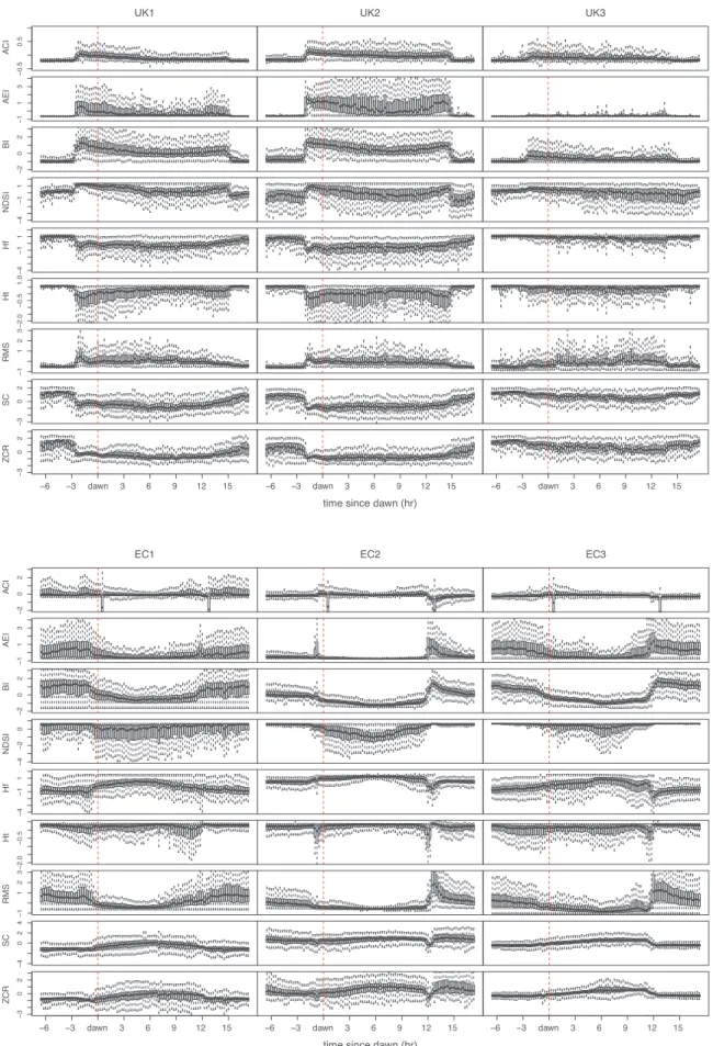
Examination of the response of AIs to diurnal changes in acoustic activity seen in the full data set helps to interpret the results of the correlation analyses of the labelled subset, including the negative cor-relations observed for the entropy indices. Diurnal soundscape patterns

[3]

https://github.com/patriceguyot/Acoustic_Indices.

Calculations were carried out using a bespoke python library to facilitate rapid computation [3]. Indices in categories 1–5 were based on implementations in the seewave library (Sueur et al., 2008) [1] and soundecology [2] R packages; results from the python library were validated experimentally to ensure absolute equivalence with the R packages. For indices in categories 2–5 a single value was calculated for each 1 min ﬁle. Indices based on frequency analyses (1–5, 7) were calculated from a spectrogram computed as the square magnitude of an FFT using window and hop size of 512 and 256 frames respectively. Indices based on short sections (frames) of audio (1, 6, 7, 8) were cal-culated for 512 samples. Mean, variance, median, minimum or max-imum are recognized to track diﬀerent facets of the acoustic environ-ment; each of these 5 statistical variants were calculated for frame-based indices (ACI, SC, RMS and ZCR) giving a total of 26 indices. 2.6. Baseline avian diversity

Baseline community measures of diversity and abundance (Santini et al. 2016) were calculated for the subset of labelled data. Avian, amphibian and insect densities were compared per habitat type and registers of other vocalizing species recorded.

2.7. Statistical analyses

2.7.1. Do AIs track changes in avian diversity?

Three aspects of avian diversity were evaluated i) changes in species richness and abundance across sample points; ii) diurnal variation in vocalization density; iii) habitat dependent variation in community composition.

2.7.1.1. Correlation Analyses (Q1 a). To test the relationship between each of the AIs, and avian species diversity and biophonic diversity across all sample points, two-tailed Spearman's rank correlations were carried out between each of the 26 AIs, species richness, species abundance and biophonic density (BD). In line with previous research (Mammides et al., 2017) species richness (N0) was seen to correlate strongly with abundance (NN) in both ecozones, presumably due to short survey times, so further analyses were carried out using N0 only. 2.7.1.2. Time series plots (Q1 b). In order to observe how AIs relate to a gradient of vocal community density, time series plots of the full data set were made; AI values (1 min every 15) for each channel over each of the 10 sampling days were calculated and plotted relative to dawn for each of the 15 sample sites at each habitat (28,800 values per habitat per ecozone).

2.7.1.3. Multivariate Classification (Q1 c). To evaluate whether AIs reflect observed differences in community composition between habitats, clustering analyses were performed on species abundance data and AIs for the labelled data (UK = 1976, EC = 1201). A multivariate random forest classifier (MRF) (Breiman, 2001) was built for each ecozone, with habitat type as response and either species relative abundance (EC = 90, UK = 65) or AI (n = 26) as predictors. The out of bag (OOB) error rate gives the MRF predictive power and OOB confusion matrices obtained from the MRF predictor. Error rates are taken as a measure of how distinct each habitat is, in terms of either avian community composition or acoustic environment.

2.7.2. Are compound indices more powerful than any single metric? 2.7.2.1. Multivariate regression analyses (Q2). To test whether compound indices are more powerful predictors of avian species richness than any single AI, and to investigate the relative contributions of each, a multivariate random forest regression model

(8)

in all habitats are clearly observable in the temporal variation of AI values over 24 h periods (Fig. 6). UK nights (Fig. 6top) are quiet re-lative to day time avian activity: this is seen in low nocturnal values of ACI, AEI, BI and RMS. Entropy indices (ADI, Hf and Ht), SC and ZCR show the reverse pattern, as per correlation results. In contrast, Ecua-dorian nights (Fig. 6bottom) show an increase in acoustic activity. Peak activity at dawn and dusk anuran choruses are clearly visible as strong peaks in the AEI, inverted in Ht.

3.1.3. Classiﬁcation analyses

Overall, errors were lower for multivariate classification by AIs than by species in both the UK and Ecuador (Fig. 7right versus left, top and bottom) but follow the same pattern or relative magnitudes. This sug-gests that differences in acoustic environments between sites are greater than inter-site differences in community composition but track changes in community composition: Errors for UK by species are lowest for UK3 (5%) compared to the two forested habitats UK1 (15%) and UK2 (22%); classifcation errors by AIs, are lowest of UK3 (3%), suggesting that UK3 has the most distinct soundscape as well as the most distinct avian community.

For Ecuador, errors for classiﬁcation by species were lowest in EC1 (1%) with higher errors in EC2 (18%) and EC3 (21%), suggesting that there are more shared species between EC2 and EC3 than in the primary forest of EC1. Similarly, errors for acoustic indices are negligible for each habitat in Ecuador (1%, 3% and 1% respectively), suggesting soundscapes at each site are highly distinct.

3.2. Multivariate random forest regression analyses

MRF regression analyses confirm that compound indices are stronger predictors of species richness than any single index: BI is the strongest single predictor of N0 in both UK (34% variance explained) and Ecuador (13% variance explained) (Fig. 8). For the UK, AEI also makes a significant contribution (18%), followed by ACI.med, ACI, ADI, ACI.min, ACI.max and ZCR.mean, NDSI and ACI.var. In Ecuador, the simple acoustic descriptors make significant contributions: ZCR.mean accounts for an additional 13% variance, followed by SC.max, NDSI, ZCR.med, ACI.var and RMS.var. All other indices exceed the analytic threshold (Ishwaran et al., 2010), suggesting that they all make a contribution to predictive power, however small. These results clearly demonstrate that a compound index has more predictive power than any single AI alone. Partial dependence plots which elucidate the nature of these relationships are given inSupplementary materialE.

4. Discussion

The observed correlations between species richness and AIs in temperate habitats approach the strengths expected for AIs to be adopted as indicators of biodiversity and are stronger than those re-ported in recent smaller scale terrestrial correlation studies. Thus al-though it has been suggested that there are many other sources of acoustic heterogeneity that could undermine the value of AIs as proxies for biodiversity (Gasc et al., 2013), the present results suggest that with Fig. 3. Tukey’s box plots of avian species richness per sample site for each habitat in UK (left) and Ecuador (right). The highest median avian species richness per sample site was observed in secondary habitats in both ecozones. Horizontal lines represent medians; the box represents the interquartile range; whiskers represent min and max values within 1.5 IQR. Shapiro-wilk normality test showed neither data set to be normal (UK W = 0.966, p < 0.0001; EC W = 0.968, p < 0.001). Non-parametric two sample tests confirmed observed differences in species rich-ness between each habitat in the UK to be significant (p < 0.001); in Ecuador richness in both secondary forest and agricultural plantation was significantly greater than in the primary (p < 0.001), but differ-ences between secondary and agricultural habitats were non-significant (p = 0.175). See supplementary material C for full details.

UK Avian BD EC Avian BD EC Amphibian BD EC Insect BD

Fig. 4. Box and whisker plots for multi-taxa biophonic density (BD) per sample site. Horizontal lines represent medians; the box represents the interquartile range; whiskers represent min and max values within 1.5 IQR. For the UK (far left) biophonic density is equal to the percentage acoustic cover per 1 min ﬁle of avian vocalisations. Each band is assigned a value 0–3 for analysis. For Ecuador (right) BD includes avian, amphibian and invertebrate vocalisations and is calculated as the average score for each 1 min ﬁle.

(9)

suﬃcient spatial and temporal replication these local individual dif-ferences may be ameliorated by community level eﬀects.

We report five key findings which contribute to the interpretation, development and application of acoustic indices for biodiversity mon-itoring in the future: i) Vocalising species richness does not necessarily increase with ecological status ii) AIs track changes in acoustic com-munity composition and reveal strong differences in acoustic environ-ments between habitats iii) AIs correlate strongly with vocalising avian species richness in temperate (mono-taxa) environments and with subjective measures of biophonic density in both tropical and temperate ecozones; iv) Performance of simple acoustic descriptors approaches that of bespoke diversity indices across ecological conditions and con-tributes more to predictive power than most diversity indices in multi-taxa environments; v) compound indices are more effective than any single index in predicting species richness.

4.1. Vocalising avian species richness does not increase with habitat status Registered avian species richness was signiﬁcantly higher in the secondary habitats than the ancient temperate and primary tropical forests. The relationship between habitat status and species diversity was not a central question of the current study, but a positive re-lationship between habitat status and acoustic diversity is a founda-tional assumption of RAS (Sueur et al., 2008) and ecoacoustics (Villanueva-Rivera et al., 2011). Our results challenge this assumption and are in line with previous studies: a similar pattern was observed in a study in the Ecuadorian Cloud Forest (Eldridge et al., 2016); greater diversity has also been reported in young, evolving forests compared to mature forests (Depraetere et al., 2012); and recent studies evaluating the relationship between soundscape and landscape in Australian Gum forests similarly ﬁnd no clear, positive relationship between biocondi-tion and species richness (Fuller et al., 2015). That the secondary forest sites show greater avian species richness is not unexpected: all ex-hibited over a decade of regrowth, providing a range of niche space for

a wide diversity of avian species (Reid et al., 2012). More generally, it is recognized that high diversity does not ensure that a site has a high ecological value (Dunn, 1994), and that species richness alone may not be suﬃcient to fully understand ecosystem resilience and functioning (Chillo et al., 2011). Therefore, the assumption that acoustic di-versity is a proxy for habitat health may be questioned.

4.2. AIs track changes in community composition and reveal strong diﬀerences in acoustic environments between habitats

Multivariate classification analyses showed that AIs follow the same pattern of change across habitats as species composition; errors for classification by AIs were even smaller than errors by species lists, suggesting that between habitats differences in acoustic environment are even greater than differences in acoustic community composition. The ecological relevance of these differences is unclear but warrants further investigation. Explanations include: i) differences in vocaliza-tion characteristics of registered species. For example, the agricultural land in the UK differed from the forest sites in the presence of skylarks and absence of pheasants, both species having very distinct calls which strongly impact many of the indices values; ii) Prevalence of non-avian taxa. As seen inFig. 4there were marked differences in anuran and invertebrate activity across sites; iii) site-specific differences in an-throphonies such as airplanes, generators or human voice; iv) site-specific differences in geophonies (wind, rain), potentially augmented by the impact of habitat structural variation on propagation of acoustic signals. These results tentatively point to the possibility thatacoustic assessments could potentially provide a more complete measure of biodiversity than traditional avian surveys; further research should investigate the potential for acoustic assessment of community com-position and ecologically relevant differences in acoustic environments. Fig. 5. Spearman’s rank coefficients for correlations between each acoustic index and species richness (left) and biophonic density (right) for UK (top, N = 1976) and Ecuador (bottom, N = 1201). Stars denote p-values (***_{< 0.001,}**_{< 0.01,}*_{< 0.05, . < 0.01), textures group class of index.}

(10)

Fig. 6. Main AI values for each 1 min ﬁle for all 15 sample sites averaged over 10 days in each UK (top) and EC (bottom) habitat type and plotted relative to dawn (vertical dashed line). Central band shows mean and standard deviation; IQR is denoted by dashed lines. N = 28,800 per habitat.

(11)

4.3. AIs correlate with vocalising avian species richness in temperate (mono-taxa) environments

Strong correlations were also observed between AIs and subjective measures of biophonic density in both tropical and temperate ecozones. Overall, we observe stronger relationships between AIs and species richness in temperate habitats than have been reported in recent cor-relation studies, possibly because these previous studies were carried out in tropical environments where results may have been confounded by other vocalizing taxa. This interpretation is supported by the fact that AIs correlate signiﬁcantly with the subjective multi-taxa measure of biophonic density in both ecozones in the current study.

These results suggest ﬁrstly that AIs successfully track acoustic communities, (even in the presence of considerable anthrophony and geophony), and secondly reiterate the need to develop and test acoustic methods to assess multi-taxa communities.

Observed relationships between avian species richness and BI, ACI and NDSI are largely in line with previous ﬁndings. In contrast, entropy and evenness indices (AEI, ADI, Hf, Ht) show an inverse relationship to many previous ﬁndings. Results for each class of index are discussed below:

•

The Bioacoustic Index showed the best overall performance, being the strongest predictor of avian species richness in both ecozones and showing strong positive correlations with species richness in the UK and biophonic density in Ecuador and the UK. This result cor-roborates previous studies which report strong correlations between BI and avian species abundance (Boelman et al., 2007), number of bird vocalizations (Pieretti et al., 2011) and biotic diversity (Fairbrass et al., 2017). The superior performance of BI over other indices could be attributed to the fact that it is calculated across a

narrower frequency range, potentially strengthening the relation-ship with biophony by reducing sensitivity to low frequency engine and wind noise and high frequency components of insect calls. This is a simple but important considering in the design of future indices. Future indices could be band limited and tuned to the range of calls of interest.

•

Correlations between ACI and species richness in the UK are in line with many previous ﬁndings which report positive relationships between ACI and number of avian vocalisations (Pieretti et al., 2011) and reef ﬁsh abundance in temperate (Harris et al., 2016) and tropical (Bertucci et al., 2016) marine environments. The weaker relationship between ACI and observed species richness and nega-tive relationship to biophonic diversity in Ecuador is understandable given the other biophonies present: ACI acts as an event detector, so it will likely track insect and amphibian calls with rapid onsets; si-milar negative trends have recently been reported in other areas of high species diversity (Mammides et al., 2017). It is of note but not surprising that median values performed a little better than the standard mean value, being less susceptible to extreme changes which may be due to wind, electronic error or other biasing outliers. Median, rather than mean values may be more robust metrics in general.

•

Although NDSI was developed to capture anthropogenic dis-turbance, rather than acoustic community diversity, significant re-lationships with bird species richness have been reported elsewhere (Fuller et al., 2015), however weak and non-significant correlations have also been observed (Mammides et al., 2017). The moderate, positive correlations observed here between species richness and biophonic density likely reflect an overall increase in biophonies relative to background technophonies – which were present in all habitats here – supporting the use of NDSI as a high-level measure of Fig. 7. Confusion matrices for multivariate classifi-cation of habitat by species (left) and acoustic indices (right); actual habitats are shown in columns and predictions as rows for EC (N = 1201: 424, 420, 357) and UK (N = 1976: 663, 645, 668). Overall OOB classification errors are shown in each subplot title, and error rates per habitat type on the x-axes.

(12)

anthropogenic disturbance. As has been highlighted elsewhere, as-sumptions over frequency range of anthrophony and biophony may be over simplistic: frequency components of anthropogenic and biotically generated sounds are not necessarily strictly band-limited, but could potentially be tuned to meet local characteristics. For example, calls of the Ecuadorian Toucan barbet (Semnornis ram-phastinus) contain spectra as low as 300 Hz, well below the default 2 kHz lower limit of biophony in NDSI.Ranges for frequency-de-pendent indices could be tuned to particular characteristics of local communities of interest.

•

The Acoustic Evenness Index (AEI) showed the highest correlation with species richness in the UK and contributed strongly to predic-tion in the multivariate regression model. The observed strong po-sitive correlations between species richness and Acoustic Evenness Index and negative correlations between species richness and the entropy indices show that evenness of the spectra decrease with in-creasing richness for ADI, Ht and Hf. These ﬁnding are at odds with some previous short term correlation studies, but show the same

patterns observed in longer term soundscape investigations (Gage and Farina, 2017) and shed light on inconsistencies previously re-ported for entropy indices (Depraetere et al., 2012; Sueur et al., 2014). Given that the measurement of acoustic diversity is founda-tional to RAS, reconciling these inconsistencies is important, as conﬂicting accounts exist both empirically and hypothetically. 4.3.1. Interpretation of entropy indices

AEI, ADI and Hf are derived by calculating Gini and Shannon in-dices on the relative distribution of acoustic energy across frequency bands in a given recording. The motivational logic is that an increasing number of species will generate signals across a wider range of fre-quencies due to partitioning (Sinsch et al., 2012; Sueur, 2002), resulting in increased evenness (AEI tends to zero and ADI and H to 1). However, this is only true over the bandlimited range of bird song (often cited as 2–8 kHz). Over a wider frequency range, the inverse prediction also stands: as the mid- and high-frequency range of songbird vocalisations increase relative to acoustic energy at the top and bottom of the Fig. 8. Cumulative percentage variance explained by multivariate random forest regression model using all 26 AIs as predictors of N0 for UK (60% variance explained, error rate = 3.28%, top) and EC (47% variance explained, error rate 2.65%, bottom). AIs are ordered by minimal depth.

(13)

that they are likely to be less biased by dominant species vocalisations. Some indices are particularly sensitive to certain call characteristics, compromising their reliability as a biodiversity proxy. For example, we have noticed in previous work that the high frequency short, rapid shrill of the Dusky Bush Tanager (Chlorospingus semifuscus) generates high ACI values.The ﬁrst generation of ecoacoustic indices aimed to provide single values of acoustic diversity; future research should focus on development and testing of a suite of complementary features for use in a compound index, capturing timbral as well as temporal and spectral characteristics. Site-speciﬁc compound in-dices could then be developed, for example by tuning relative weights by carrying out a PCA on a sample recording.

4.6. Future directions in acoustic indices

The development of indices for RAS in multi-taxa environments can be approached under one of two principles: either focusing on a single identiﬁed indicator taxon (birds or amphibians) and removing un-wanted sounds (insect choruses, wind rain); or attempting to capture the global interplay of multi-species, multi-taxa choruses. Exciting ad-vances are being made in both areas using machine learning: source separation algorithms can be used to tackle the former (Xie et al., 2016), and unsupervised clustering algorithms have been productively applied to analyse the variety of sounds sources in long term mon-itoring projects (Phillips et al., 2018). Whilst powerful these approaches are too computationally intensive to run on microcomputers in situ. The use of simple acoustic descriptors which track changes across spectral, temporal and timbral dimensions of vocalisations oﬀer an alternative, parsimonious approach to monitoring the integrated chorus and point to new directions for the development of tuneable, compound ecoa-coustic indices capable of tracking the dynamics of multi-taxa aecoa-coustic communities.

5. Conclusion

Results from acoustic surveys across a wide range of ecological conditions, in temperate and tropical ecozones support the use of acoustic indices to appraise avian species richness in temperate but not in the multi-taxa acoustic communities of tropical habitats. Compound indices appear to be sensitive to habitat-dependent changes in acoustic community composition, which could provide a potentially more cost-effective and nuanced assessment than current standard avian surveys against which we are validating. These results both highlight the need for, and inspire the development of, new indices for monitoring more complex multi-taxa communities. Our results clearly demonstrated that compound indices are to be recommended, and that development and testing of new simple timbral, spectral and temporal indices to com-plement existing diversity indices deserves further investigation. Future research should confirm these results and further integrate extant knowledge from machine listening and bioacoustics research to create more powerful computational methods for the analysis of acoustic community dynamics at extended spatio-temporal scales. By doing so we can maximize the potential for ecoacoustics methods to provide robust, cost-effective tools for ecological monitoring and prediction. Acknowledgements

Joseph Cooper and Manuel Sanchez for avian species identification in UK and Ecuador respectively, Penny Green and Jorge Noe Morales for verification. For support in field surveys Claire Reboah, Josep Navarro, Galo Conde, Wagner Encarnacion and Raul Nieto. For access to UK field sites, all at Plashett Park Wood, especially Mike Cameron, all at Knepp Wildland Estate, especially Penny Green and for access to Tesoro Escondido, Citlalli Morelos, the community of Tesoro Escondido and the Cambugan Foundation. Thanks for anonymous reviewers for swift and productive feedback on an earlier version of this manuscript. spectrum, evenness would decrease (AEI tends to 1). Therefore, both the

strength and direction of relationship between biophonic diversity and entropy indices is related to the frequency range analysed.

The bimodal response of entropy indices also makes interpretation difficult. Entropy metrics in both time and frequency domains report high values for signals with diametrically opposed acoustic and ecolo-gical characteristics: As noted in the seewave documentation, the temporal entropy of signals of high acoustic activity (with many am-plitude modulations) and a quiet signal will both tend towards 0, but a sustained sound with an almost flat envelope will also show a very high temporal entropy. Similarly, for any given frequency range, the spectral entropy of a signal of high acoustic activity and diversity (lots of species calls across different frequencies) will produce a high value, whereas the call of a single species will produce an isolated spike and a low value. However, recordings with very low acoustic activity and low signal:noise ratio will also result in a high diversity value due to the low magnitude, flat spectra. Entropy indices have a bimodal, rather than unimodal response. Thus, whether ADI and AEI decrease or increase with increasing species richness depends on whether you compare high activity either to silence or low activity, i.e. the length of acoustic density gradient. Inconsistencies in results for H indices have previously been attributed to the presence of technophony (plane, car, farm ma-chinery or train) (Depraetere et al., 2012) which produce a flat spec-trum similar to the broadband white noise of silence. The sampling regime deployed here highlights that low signals (silence) gives similar results. Thus, when a long gradient of vocalization density is included in the sampling protocol, inequality and entropy decrease with species richness, in direct contrast to standard ecological interpretations of Gini-Simpson and Shannon-Wiener indices when applied to species counts. Entropy indices are non-intuitive and must be interpreted carefully.

4.4. Performance of simple acoustic descriptors

The performance of simple acoustic descriptors RMS, ZCR and SC suggest alternatives to single temporal or spectral diversity metrics and inspire further research in the development and testing of acoustic in-dices. Correlation strengths of RMS, ZCR and SC approached that of the diversity indices and, in Ecuadorian habitats, ZCR and SC made sig-nificant contributions to species richness predictions. As expected, RMS shows a positive association with increasing vocal activity and ZCR and SC are negatively associated. Rather than measuring acoustic diversity, these simple descriptors track changes in amplitude (RMS), spectral (SC) and temporal characteristics of signals (ZCR). RMS and SC are intuitive to interpret; the contribution of ZCR to predicting avian richness in complex multi-taxa environments can be understood in light of its recognized power in percussion classification tasks. The ZCR of the decay portion of percussive sounds is reported to out-perform more complex computations in separating the high pitch sharp attacks of snare drum hits from lower frequency, slower onset, bass drum strikes (Gouyon et al., 2002). The possibility that such a simple descriptor may track distinct characteristics of the vocalisations of different taxa – such as the rapid onset of harmonic bird vocalisations versus the continuous noise of some invertebrates – warrants further investigation. Compu-tational simplicity translates to low energy requirements, making these simple descriptors ideal candidates for implementation of in situ ana-lysis for the emerging generation of monitoring networks built from the emerging generation of embedded devices.

4.5. Compound indices are more eﬀective than any single index in predicting species richness.

Multivariate regression results demonstrating the superior perfor-mance of compound over single indices are in line with results of pre-vious studies (Wimmer et al., 2013) and follow intuition. Besides in-creasing predictive power, another advantage of compound indices is