OATAO is an open access repository that collects the work of Toulouse
researchers and makes it freely available over the web where possible
Any correspondence concerning this service should be sent
to the repository administrator:
tech-oatao@listes-diff.inp-toulouse.fr
This is a publisher’s version published in:
http://oatao.univ-toulouse.fr/26714
To cite this version:
Rousseau, Lola and Rouzaud, Olivier and Lempereur,
Christine and Orain, Mikael and Simonin, Olivier Influence of
droplet spatial distribution on spray evaporation. (2019) In:
ILASS–Europe 2019, 2 September 2019 - 4 September 2019
(Paris, France).
Official URL:
https://ilass19.sciencesconf.org/browse/author?authorid=678735
Open Archive Toulouse Archive Ouverte
Influence of droplet spatial distribution on spray evaporation
Lola Rousseau*
1, Olivier Rouzaud
1, Christine Lempereur
1, Mikael Orain
2, Olivier Simonin
3 1ONERA, Centre Midi-Pyrénées, Toulouse, France
2
ONERA, Centre Midi-Pyrénées, Fauga-Mauzac, France
3
Institut de Mécanique des Fluides de Toulouse (IMFT), Université de Toulouse, CNRS,
INPT, UPS, Toulouse, FRANCE
*Corresponding author:
lola.rousseau@onera.fr
Abstract
In aero-engines, fuel is injected as a liquid which involves two-phase flow combustion. Consequently, different phenomena such as atomization, droplet dispersion by turbulence or spray evaporation impact combustion processes. In order to study spray combustion, an experimental test rig has been developed at ONERA to partially feature the flow conditions inside the combustion chamber of a turbo-reactor. Experimental campaigns have been conducted in non-reactive and reactive conditions to obtain an experimental database. The present paper focuses on the correlation between droplet density and the nearest-neighbour droplet distance obtained from the analysis of Mie scattering images under non-reactive conditions. Results show that the nearest-neighbour droplet distance varies linearly with the inverse square-root of mean spray density. Findings are compared with the theoretical law of Hertz-Chandrasekhar and the regular arrangement law.
Keywords
Combustion, Evaporation, Inter-droplet distance, Spray Introduction
Gaseous combustion inside a combustion chamber has been studied for decades due to its importance in several applications. In aeronautics, liquid fuel is injected inside the engine combustion chamber. In such flows specific phenomena occur such as atomization, droplet dispersion or evaporation. Since combustion occurs in the gaseous phase, the global behaviour of spray in evaporation is of particular importance. Furthermore, collective effects between droplets may play a major role on this behaviour.
Seminal works of Godsave [1] and Spalding [2] concern the evaporation and combustion of an isolated fuel droplet. These papers developed a theoretical model which was compared to experimental results. Ever since, a very large number of articles have dealt with the combustion of an isolated droplet, including the different shapes of the flame front around the droplet [3], [4]. Beck et al. [5] showed that, in a very dilute spray, droplets burn individually according to two flame types: an envelope flame surrounding the droplet or a wake flame behind the droplet. Nonetheless, the isolated droplet model may not be representative of a dense spray where droplets can be close to each other. For this reason, in the eighties, several research groups developed theoretical concepts of droplet group combustion. For example, Chiu et al. [6] proposed a model of spray with regularly distributed droplets (distance deduced from the density of the spray). In this model, four spray combustion regimes were proposed and the combustion regime was determined from the group combustion number G defined by:
𝐺𝐺 =1.5𝐿𝐿𝐿𝐿 ∗ �1 + 0.276 ∗ 𝑆𝑆𝑐𝑐 1
3∗ 𝑅𝑅𝐿𝐿12� ∗ 𝑁𝑁23∗ 𝑑𝑑 𝐷𝐷𝑖𝑖 (1)
where Le, Sc, Re are respectively the Lewis number, the Schmidt number and the Reynolds number, N represents the total number of droplets contained in the group, d is the droplet diameter and 𝐷𝐷𝑖𝑖 equals the mean distance between droplet centres. The work of Kerstein et al [7], subsequently used by Borghi and Champion [8], offered another description for spray combustion in a premixed flow. This model is based on the following criterion:
𝑆𝑆 = 𝑛𝑛13∗ 𝑟𝑟𝑓𝑓=𝑟𝑟𝑓𝑓 𝛿𝛿𝑠𝑠 (2)
where nis the droplet density,𝑟𝑟𝑓𝑓 is the radius of the flame which surrounds a droplet and 𝛿𝛿𝑓𝑓 is the droplet inter-distance. The value of S defines the combustion regime. For 𝑆𝑆 < 0.41, the configuration corresponds to a dilute spray where droplets burn as a group. As the value tends to zero, the number of droplets surrounded by the flame becomes smaller and smaller, which leads to an isolated droplet combustion regime. For 𝑆𝑆 > 0.73, the configuration is that of a dense spray where pockets of gas are surrounded by flames. In the intermediate combustion mode, both previous regimes coexist.
ILASS – Europe 2019, 2-4 Sep. 2019, Paris, France
On the experimental side, the influence of droplet spacing on droplet evaporation and combustion was first investigated using linear arrays of droplets [9], [10]. Later on, complexity was added by studying droplet sprays. For example, Chen and Gomez [11] studied a laminar spray flame of heptane droplets and have confirmed the existence of different group combustion regimes in the spray and the transitions between the various regimes. Akamatsu et al. [12] used a coaxial configuration with the injection of liquid kerosene to observe different spray combustion regimes by means of various optical diagnostics. Results partially validate Chiu’s theoretical model, discrepancies between experiments and theory were attributed to the fact that the droplet spatial distribution in the spray is non uniform as opposed to that in the model developed by Chiu et al. [6]. Nevertheless, only a few studies have investigated the influence of droplet spacing on the evaporation of a realistic spray. Again, such studies were first performed on droplet streams. Recently, Sahu et al. [13] used laser diagnostics to investigate a non-evaporating water spray and an evaporating acetone spray at atmospheric pressure and ambient temperature. Correlations between spray density, vapour mass fraction, droplet size and velocity have been identified and an estimation of a group evaporation number, in reference to Chiu’s group combustion number, is provided.
While the distance between the droplets is an important parameter for modelling droplet evaporation, the spatial distribution of droplets within the spray is also a point of interest for that purpose. In Chiu’s theory, the droplets are supposed to be regularly arranged in the spray. Nonetheless, there are other scientific fields such as meteorology where the Hertz-Chandrasekhar law is commonly adopted, although a certain number of works question its relevancy [14]. Assessing this law in droplet sprays might be interesting and this may help to provide a better modelling of real sprays. Additionally, preferential segregation due to coherent structures in the flow may lead to the clustering of particles [14], [15] and this phenomenon shall be addressed as well.
An experimental test rig has been developed at ONERA to study such behaviour under non-reactive and reactive conditions, the PROMETHEE test rig (Vicentini [16]). Several optical devices have been employed to characterise the two-phase flow. In particular Mie scattering images were used to determine the spatial distribution of the spray and the droplet nearest-neighbour distance under reactive conditions. A specific image processing algorithm has been developed to study the spray behaviour under non-reactive conditions. It enables to calculate stationary and phase-averaged values of local spray density and droplet nearest-neighbour distance.
While some results from the reactive case [16], [17] will be recalled, this paper focuses on the non-reactive case. In the second part of the paper, the experimental test rig and data set are described. Then, the processing algorithm for Mie scattering images is detailed. In the fourth part, spray density for both stationary and phase averaging methods will be compared and the nearest-neighbour inter-droplet distance will be studied as a function of the spray density. A comparison with the theoretical law of Hertz-Chandrasekhar [18], [19] and the regular arrangement law will also be provided.
Material and methods
Experimental test rig and operating conditions
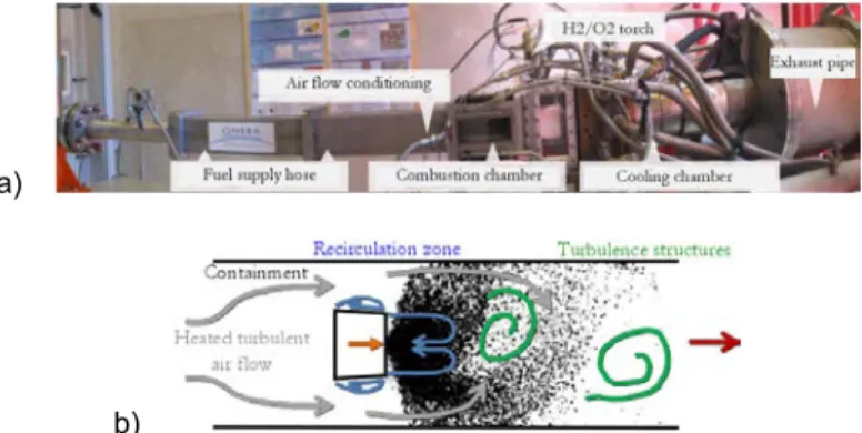
With the aim of studying spray combustion, the PROMETHEE experimental test rig (figure 1.a) has been developed at ONERA. The design aims at reproducing part of the flow conditions met inside the combustion chamber of a turbo-reactor. The internal section of the combustion chamber is equal to 120 x 120 mm². A trapezoidal bluff-body which allows a 42 % blockage ratio is located in the channel in the span-wise direction. A recirculation zone develops downstream from the bluff-body and, for non-reactive conditions, a vortex-shedding phenomenon is observed in the chamber (figure 1.b). The fuel injection system consists of a flat-fan nozzle fixed at the rear of the bluff-body, on its axis, which creates an elliptical-shaped polydisperse spray of droplets. A hydrogen-oxygen torch is used to ignite the fuel-air mixture and the burnt gases are ejected into the exhaust pipe. Walls of the combustion chamber have been equipped with UV-transparent windows to allow optical measurements performed downstream from the fuel injector.
a)
b)
Air and fuel mass flow rates are respectively equal to 58 g/s and 1 g/s and the fuel/air equivalence ratio is around 0.24. The air flow is at atmospheric pressure and heated at 450 K. Liquid fuel injected on the combustion chamber is n-decane and its initial temperature is equal to 330 K. The mean flow velocity is equal to 5.8 m/s and the Reynolds number based on the height of the bluff-body is about 22 000.
Optical measurement techniques and pressure measurement
The PROMETHEE test rig has been developed with the purpose of creating an exhaustive experimental database to better understand spray evaporation and combustion and to validate numerical simulations. To this end, several optical measurement techniques have been implemented. Mie scattering is employed to determine spatial droplet distribution in the spray. Phase Doppler Interferometry (PDI) enables to measure droplet speed and diameter. OH-chemiluminescence and OH-Planar Laser-Induced Fluorescence (OH-PLIF) methods are used to locate and study the flame front for reacting conditions. Particle Image Velocimetry is used to characterize velocity fields. Finally, pressure measurement allows understanding flow instabilities which take place in the combustion chamber (figure 1.b). Later in this paper, only Mie scattering images and pressure signals are analysed.
The Nd:YLF Quantronix laser (λ = 527nm) produces the light sheet which illuminates the droplet spray in the combustion chamber. The frequency is 1 kHz and the laser pulse is about 200 ns. Mie scattering images of droplets are acquired with a Phantom V341 high-speed camera. A differential pressure signal is measured by a Validyne sensor which is located on the bluff-body. For more details about the experimental setup, the operating conditions and optical measurements, the reader can refer to the article of Rouzaud et al [17].
Mie scattering database
Around 4000 raw images have been collected for each operating point. In order to have the best possible spatial resolution, either the upper part of the flow or its lower part half has been visualized (figure 2). The image definition is 1800 x 1600 px ² and it covers an area of 51x 46 mm², so that the image resolution is roughly 35 pixels per mm. While images for the reactive case represent both parts of the combustion chamber, images recorded for the non-reactive case represent only upper part (grey area in figure 2).
Figure 2. Location of Mie scattering images with respect to the injector body
Data averaging
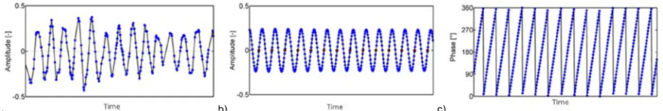
There are two ways of calculating mean values. On one side, a stationary average value is obtained for each pixel and is based on an arithmetic average on the whole set of images. Such a process applies to reactive and non-reactive data. On the other side, and only under non-non-reactive conditions, phase averaging is possible thanks to a reference signal. In that case, a von Karmàn vortex street appears behind the bluff-body and its presence is clearly exhibited by the pressure measurement of the Validyne sensor providing the differential pressure between the upper and the lower walls of the obstacle (figure 3.a). Using this periodic signal as a reference, such a measurement enables to sort the whole set of Mie images with respect to time. Since the vortex shedding involves a periodic variation of the differential pressure signal, applying a Fourier transform to this signal from which the mean value has been subtracted provides the main signal frequency. After applying a Butterworth filter centred on the main frequency, it is possible to determine the zero crossings of the signal (figure 3.b). The combination of zero crossings and image acquisition time allows allocating a specific phase to each image. The next step consists in discretizing the phase space in a limited number of bins of length ΔՓ. The choice of this value necessitates a trade-off between time accuracy and a sufficient amount of data to perform averaging. Vicentini [16] has shown that a value of 4° is sufficient enough to obtain consistent results when processing PIV images. Finally, phase averaging is performed by taking into account all the images of each specific phase interval. Obviously, phase average study is only possible for non-reactive conditions. In this process, the number of images per phase interval is generally around 80 for the retained value of ΔՓ.
ILASS – Europe 2019, 2-4 Sep. 2019, Paris, France
b) c)
Figure 3. Profile of pressure signal. a) initial signal. b) filtered signal. c) zero crossings according to acquisition time. Lenght of a
period is around 1
33 s.
Mie scattering image processing Values of interest
In order to describe the spray behaviour, two specific geometrical parameters have been selected. The first one corresponds to the spray density 𝑛𝑛(𝑥𝑥, 𝑦𝑦) which is the number of droplets per square centimetre relative to the pixel (x,y). The second parameter corresponds to the nearest-neighbour inter-droplet distance which represents the smallest distance between a droplet “g” in the spray located at pixel (x,y) in the i-th image and its nearest neighbour “g*”. It is defined as the Euclidian distance:
𝑑𝑑𝑛𝑛𝑛𝑛𝑖𝑖(𝑥𝑥, 𝑦𝑦) = ��𝑥𝑥
𝑔𝑔− 𝑥𝑥𝑔𝑔∗�² + �𝑦𝑦𝑔𝑔− 𝑦𝑦𝑔𝑔∗�2 (3)
By convention, 𝑑𝑑𝑛𝑛𝑛𝑛𝑖𝑖(𝑥𝑥, 𝑦𝑦) is equal to zero when there is no droplet present at pixel (x,y).
For each image set, a phase averaging step is carried out. An occupancy rate OR is defined as the sum of the occurrences of a droplet at a given pixel calculated from all the images 𝑁𝑁𝑖𝑖 of the set. 𝑔𝑔𝑖𝑖 is equal to zero when there is no droplet in the pixel (x,y) for image “i” and one when a droplet is located on this pixel. Thus, the occupancy rate is obtained as:
𝑂𝑂𝑅𝑅(𝑥𝑥, 𝑦𝑦) = � 𝑔𝑔𝑖𝑖(𝑥𝑥, 𝑦𝑦) 𝑁𝑁𝑖𝑖
𝑖𝑖=1
(4)
For instance, if the image set contains 𝑁𝑁𝑖𝑖 images and a droplet is detected in the pixel (x,y) three times, its occupancy rate will be equal to three. Thus, the average value of the nearest-neighbour inter-droplet distance for each specific phase value is defined as follows:
𝑑𝑑𝑛𝑛𝑛𝑛 (𝑥𝑥, 𝑦𝑦) =𝑂𝑂𝑅𝑅(𝑥𝑥, 𝑦𝑦) ∗ � 𝑑𝑑𝑛𝑛𝑛𝑛1 𝑖𝑖(𝑥𝑥, 𝑦𝑦) 𝑁𝑁𝑖𝑖
𝑖𝑖=1
(5)
The standard deviation of the nearest-neighbour inter-droplet distance is calculated in the same way.
According to Vicentini [16], [17], in the reactive case, there is a linear relationship between the mean spray density 𝑛𝑛 and the mean nearest-neighbour droplet distance 𝑑𝑑𝑛𝑛𝑛𝑛 and its standard deviation 𝜎𝜎𝑛𝑛𝑛𝑛 according to:
�𝑑𝑑𝑛𝑛𝑛𝑛(𝑥𝑥, 𝑦𝑦) = 𝛼𝛼 ∗ 𝑛𝑛−12 𝜎𝜎𝑛𝑛𝑛𝑛(𝑥𝑥, 𝑦𝑦) = 𝛽𝛽 ∗ 𝑛𝑛−12
(6)
where 𝛼𝛼 and 𝛽𝛽 are the corresponding slopes. In the case of the uniform distribution where the droplets are regularly arranged, 𝛼𝛼 equals 1 and 𝛽𝛽 equals 0. In the case of the Hertz-Chandrasekhar 2D distribution, 𝛼𝛼 is equal to 0.5 and 𝛽𝛽 is equal to 0.26. Experimental values obtained by Vicentini for 𝛼𝛼 and 𝛽𝛽 are respectively equal to 0.59 and 0.36 . For more details about results under reactive conditions, the reader can refer to [16] and [17].
Image processing algorithms
Image processing algorithms have been developed to handle Mie scattering image sets recorded in reactive as well as non-reactive conditions. An example of raw Mie scattering image is shown in figure 4.a. A top-hat filtering with a disk-shaped structuring element is firstly applied on each image to extract the droplets from an uneven background. The size of the structuring element is chosen according to the maximal size of the droplets to be detected. The 12-bit images need to be converted to binary ones prior to applying labelling functions to identify the droplets (figure 4.b). The binarization threshold must be carefully chosen in order to retain the smallest droplets. The next step is to measure geometrical parameters such as the location of droplet centres (x,y). A binary map of droplet “presence” 𝐵𝐵(𝑥𝑥, 𝑦𝑦)𝑖𝑖 is thus obtained for each image of the set (figure 4.c).This map remains a sparse matrix which will be made continuous by applying a square averaging filter in order to facilitate its
visualization and interpretation. Then, a density map which corresponds to the average over the image set is calculated as follows: 𝑛𝑛(𝑥𝑥, 𝑦𝑦) =𝑁𝑁1 𝑖𝑖� 𝑛𝑛(𝑥𝑥, 𝑦𝑦) 𝑖𝑖 𝑁𝑁𝑖𝑖 𝑖𝑖=1 (7) a) b) c) d)
Figure 4. Zoom on an image for each step of the image processing algorithm a) raw Mie scattering image b) labelled map
(color indexes the droplet number) c) Barycentre map d) density map
A parametric study on the filter size has been carried out. Figure 5 shows the density map calculated with three different sizes 𝑁𝑁𝑖𝑖 respectively equal to 25 (a), 51 (b) and 101 (c). The smallest filter size leads to a noisy map (a) whereas the enlargement of the filter size makes the images smoother (b) and (c). However, an upper limit has to be fixed to avoid smoothing too much the density in the image. Consequently, a filter size of 51x51 pixels, corresponding to a 1.5 mm-side square in the field of view has been chosen.
a) b) c)
Figure 5. Maps of mean spray density under non-reactive conditions for phase 0° with filter size of a) 25x25 b) 51x51 c)
101x101. Scale in mm
The mean nearest-neighbour inter-droplet distance map is not calculated in the same way as the density map. For the pixels where the occupancy rate is not null, the mean of the nearest-neighbour distance is calculated from all the images of the set (cf. eq. 5). To obtain a value of nearest-neighbour distance at each pixel of the map, the following filtered operation is applied:
𝑑𝑑𝑛𝑛𝑛𝑛(𝑥𝑥, 𝑦𝑦)� =∑ 𝑑𝑑𝑛𝑛𝑛𝑛(𝑥𝑥, 𝑦𝑦)𝑘𝑘 𝑆𝑆𝑓𝑓2
𝑘𝑘=1
𝐺𝐺𝑠𝑠𝑠𝑠𝑠𝑠 (8)
where 𝐺𝐺𝑠𝑠𝑠𝑠𝑠𝑠is the number of droplets contained in the filter zone. The standard deviation is evaluated in the same way.
Data convergence
The phase averaging methodology involves that the number of images per set is smaller than the one used for Reynolds averaging (around 80 images) and a convergence study has been carried out. Figure 6 presents the evolution of the mean density calculated for 0° phase for two different locations in the spray relative to areas of high (figure 6.a) and low (figure 6.b) density. A number of 80 images seems sufficient to reach a satisfactory convergence in terms of density.
a)
b)
Figure 6. Evolution of the mean density at two different locations in the spray according to the number of processed images for
ILASS – Europe 2019, 2-4 Sep. 2019, Paris, France
Results and discussion for non-reactive conditions
From now on, the results are obtained with the phase average approach at 0, 135 and 270 degrees in the upper section of the combustion chamber.
Stationary and phase average study
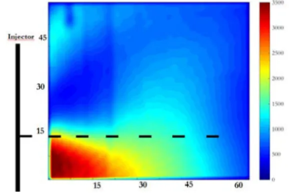
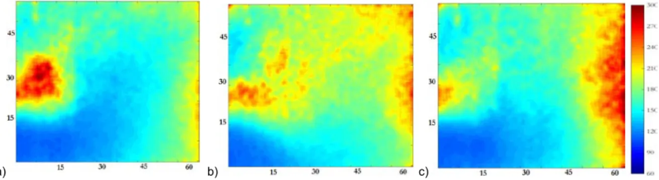
Figures 7 and 8 are pixel images of the same size and location as the grey zone in figure 2. The position of the injector (not to scale) is indicated as a black solid line in figure 7 which represents the mean spray density that ranges from 0 to 3600 droplets per square centimetre. The dashed line corresponds to the injection axis. In these experiments, the liquid injection was not symmetrical about the injector axis due to an injector defect which yields a denser region below the axis. In figure 7, the mean spray density is, as expected, more important close to the injection system while the blue regions correspond to a less dense spray. In figure 8, density maps for three different phases are shown. As expected, for all phases, the spray density is more important close to the injector and decreases with the distance to the bluff-body. Moreover, a spray flapping motion (at a frequency of 30 Hz) due to a Von Karmàn vortex shedding is captured. At zero degree (figure 8.a), part of the spray is located in the upper area of the combustion chamber and starts moving down. At 135 degrees (figure 8.b), the spray is located in the lower part of the chamber and only a small part of it is visible in this image. Finally, at 270 degrees (figure 8.c), the spray is aligned with the injection axis. Consequently, Reynolds averaging is clearly not adapted to analyse the spray behaviour under non-reactive conditions because flow dynamics and especially spray flapping motion are not captured.
Figure 7. Map of mean spray density (number of droplets per cm²) under non-reactive conditions for stationary study. Scale in
mm
a) b) c)
Figure 8. Maps of mean spray density (number of droplets per cm²) under non-reactive conditions for phase at a)0° b)135° c)
270°. Scale in mm. Nearest-neighbour distance
In figure 9, as expected, the smallest values of mean nearest-neighbour inter-droplet distance (blue regions) are located close to the rear of the bluff-body which corresponds to high spray density regions as shown in figure 9. On the contrary, when mean nearest-neighbour inter-droplet distance values increase, which corresponds to the red areas, density values decrease. For each phase, the minimum mean nearest-neighbour inter-droplet distance is around 100 µm whereas the maximum is around 350 µm. Finally, mean nearest-neighbour inter-droplet distance maps also capture the spray flapping motion.
a) b) c)
Figure 9. Maps of mean nearest-neighbour inter-droplet distance under non-reactive conditions with filter size of 51x51 pixels
for phases at a) 0° b) 135° c) 270°. Scale in mm
According to the results obtained in the reactive case, a linear relationship exists between the nearest-neighbour inter-droplet distance and the inverse of the square-root of the mean density. In order to analyse the results under non-reactive conditions, density and nearest-neighbour inter-droplet distance maps have been used to plot this last parameter versus the inverse of the square-root of the density. Figures 10 and 11 respectively present the mean and standard deviation plots for phase at 0° (a), 135 ° (b) and 270 ° (c). Colours are assigned to each point according to its occurrence. The green line represents the uniform distribution while the red line represents the Hertz-Chandrasekhar one. Several conclusions can be drawn from figure 10. Firstly, the mean nearest-neighbour inter-droplet distance seems to be linearly dependent on the inverse square-root of mean density. Secondly, for these three phases, the experimental slope is lower than those of the regular and Hertz-Chandrasekhar distributions. Moreover, most of the sample data are located between both theoretical distributions and are closer to the Hertz-Chandrasekhar one. Finally, for each phase, the mean nearest-neighbour inter-droplet distance ranges from 100 µm to 300 µm and the density values vary between 100 droplets per cm² for the most dilute part of the spray and about 3700 droplets per cm² for the densest one. Comparatively, under reactive conditions, these values are around 210 µm and 1400 µm with a spray density between 50 per cm² and 2470 per cm². From figure 11, a linear relationship is also observed between the standard deviations of these same parameters. The standard deviation value of nearest-neighbour inter-droplet distance increases when spray density decreases. For all phases, the linear relationship slope is again lower than the Hertz-Chandrasekhar distribution one but, on the contrary, sampled data are located under the results of this distribution. For these reasons, the Hertz-Chandrasekhar distribution appears as a better alternative to model droplet spray dispersion under non-reactive case than the regular distribution.
a) b) c)
Figure 10. Evolution of the mean nearest-neighbour inter-droplet distance according to the inverse square-root of mean density
for phase at a) 0° b) 135° c) 270°
a) b) c)
Figure 11. Evolution of the standard deviation of nearest-neighbour inter-droplet distance according to the inverse square-root
ILASS – Europe 2019, 2-4 Sep. 2019, Paris, France
Conclusions
Experiments performed in the PROMETHEE test rig has enabled to provide an experimental database for a two -phase flow under non-reactive and reactive conditions. In this paper, emphasis is laid on the non-reactive case. A phase averaging data acquisition process has been developed in order to describe the Von Karmàn vortex street located downstream a bluff-body. An image processing algorithm is proposed to characterize the spray behaviour in terms of inter-droplet distance and spatial distribution using Mie scattering images of the droplets. It yields maps of the density spray number, the nearest-neighbour inter-droplet distance and its standard deviation. As in the reactive case, a linear relationship is exhibited between the nearest-neighbour inter-droplet distance or its standard deviation, and the inverse of the square root of the mean density number. The spray behaviour seems to be close to the Hertz-Chandrasekhar distribution. Nevertheless, this assumption is more suitable for reactive than for non-reactive cases. This discrepancy could be explained by numerous causes like the clustering effect which could be more important under non-reactive conditions than under reactive conditions. Further work will be done to extend the experimental database and to better understand the underlying physics.
Acknowledgements
The work has been realized thanks to the partial financial support of the “Région Occitanie”. The authors would also like to thank M. Vicentini for providing these experimental data.
Nomenclature
𝑑𝑑 Droplet diameter [µm]
𝐷𝐷𝑖𝑖 Inter-droplet distance for Chiu model [µm]
𝑑𝑑𝑛𝑛𝑛𝑛(𝑥𝑥, 𝑦𝑦) Mean nearest-neighbour inter-droplet distance for pixel (x,y) [µm]
𝑑𝑑𝑛𝑛𝑛𝑛(𝑥𝑥, 𝑦𝑦)� Mean nearest-neighbour inter-droplet distance for pixel (x,y) in the continuous map [µm] 𝐺𝐺 Chiu’s group combustion [-]
𝐺𝐺𝑠𝑠𝑠𝑠𝑠𝑠 Number of droplets located in the averaging zone for nearest-neighbour inter-droplet distance map [-] 𝐿𝐿𝐿𝐿 Lewis number [-]
𝑁𝑁 Total number of droplets inside a group [-] 𝑁𝑁𝑖𝑖 Number of images contained on the image set [-]
𝑛𝑛 Mean spray density for each pixel [number of droplets per cm²] 𝑂𝑂𝑅𝑅 Occupancy rate
𝑝𝑝𝑥𝑥 Pixel [-]
𝑅𝑅𝐿𝐿 Reynolds number [-] 𝑟𝑟𝑓𝑓 Flame radius [µm]
𝑆𝑆 Criterion for Kerstein model group combustion [-] 𝑆𝑆𝑐𝑐 Schmidt number [-]
𝑆𝑆𝑓𝑓 Filter size for the nearest-neighbour inter-droplet distance map [px]
𝛼𝛼 Slope in the relationship between mean nearest-neighbour inter-droplet distance and density [-] 𝛽𝛽 Slope for standard deviation nearest-neighbour inter-droplet distance and density relationship [-] 𝛿𝛿𝑓𝑓 Inter-droplet distance for Kerstein group combustion model [µm]
𝜎𝜎𝑛𝑛𝑛𝑛(𝑥𝑥, 𝑦𝑦) Standard deviation of nearest-neighbour inter-droplet distance for each pixel [µm]
References
[1] Godsave, G.A.E., 1953, 4th Symp. On Combustion/The Comb. Institute [2] Spalding, D.B., 1953, 4th Symp. On Combustion/The Comb. Institute
[3] Jiang, T.L., and Chen, W.H., and Tsai, M.J., and Chiu H.H., 1995 , Combustion Flame, 103, 221 [4] Mercier, X., and Orain, M., and Grisch, F., 2007, Vol. 88, pp. 151-160
[5] Beck, C.H., and Koch, R., and Bauer, H.-J., 2009, 32th Symp on Combustion/the Comb. Institute [6] Chiu, H. H., and Kim, H. Y., and Croke, E. J. 1982, 19th Symp. On Combustion/The Comb. Institute [7] Kerstein, A. R, and Law, C. K., 1982, 19th Symp. On Combustion/The Comb. Institute
[8] Borghi, R., and Champion, M., 2000, “Modélisation et théorie des flammes”. Ed. Technip [9] Sommer, H.T., 1986, 21st Int. Symp. On Combustion, pp. 641-646
[10] Sangiovanni, J.J., and Labowsky, M., 1982, Combustion Flame, 47, 15 [11] Chen, G., and Gomez, A., 1997, Combustion Flame, 110, 392
[12] Hwang, S. M., and Akamatsu, F., and Park, H.-S., 2007, J. Ind. Eng. Chem.,13, pp. 206-213 [13] Sahu, S., and Hardalupas, Y., and Taylor, A. M. K. P., 2018, J. Fluid Mech., Vol. 846, pp 37-81 [14] Kostinski, A. B., and Jameson, A. R., 2000, Journal of the Atmospheric Sciences, Vol. 15, No. 7 [15] Monchaux, R., and Bourgoin, M., and Cartellier, A., 2012, Int. Journal of Multiphase Flow, Vol. 40 [16] Vicentini, M., PhD Thesis, Toulouse, 2016
[17] Rouzaud, O., Vicentini, M., Lecourt, R., Bodoc, V., and Simonin, O., 2016, 27th ILASS Conference [18] Chandrasekhar, S., 1943, Review of modern physics, Vol. 15, No. 1