O
pen
A
rchive
T
OULOUSE
A
rchive
O
uverte (
OATAO
)
OATAO is an open access repository that collects the work of Toulouse researchers and
makes it freely available over the web where possible.
This is an author-deposited version published in :
http://oatao.univ-toulouse.fr/
Eprints ID : 17215
The contribution was presented at ECAI 2016 :
http://www.ecai2016.org/
To cite this version :
Ben Amor, Nahla and El Khalfi Zeineb and Fargier,
Hélène and Sabbadin, Régis Lexicographic refinements in possibilistic decision
trees. (2016) In: European Conference on Artificial Intelligence (ECAI 2016), 29
August 2016 - 2 September 2016 (La Hague, France).
Any correspondence concerning this service should be sent to the repository
administrator:
[email protected]
Lexicographic Refinements in Possibilistic Decision Trees
Nahla Ben Amor
1and Zeineb El Khalfi
2and Helene Fargier
´ `
3and Regis Sabbadin
´
4Abstract. Possibilistic decision theory has been proposed twenty
years ago and has had several extensions since then. Because of the lack of decision power of possibilistic decision theory, several refine-ments have then been proposed. Unfortunately, these refinerefine-ments do not allow to circumvent the difficulty when the decision problem is sequential. In this article, we propose to extend lexicographic refine-ments to possibilistic decision trees. We show, in particular, that they still benefit from an Expected Utility (EU) grounding. We also pro-vide qualitative dynamic programming algorithms to compute lexi-cographic optimal strategies. The paper is completed with an exper-imental study that shows the feasibility and the interest of the ap-proach.
1
Introduction
For many years, there has been an interest in the Artificial Intelli-gence community towards the foundations and computational meth-ods of decision making under uncertainty (see e.g. [1, 28, 7, 5, 16]). The usual paradigm of decision under uncertainty is based on the Expected Utility (EU) model[18, 23]. Its extensions to sequential decision making are Decision Trees (DT) [20] and Markov Decision Processes(MDP) [6, 19], where the uncertain effects of actions are represented by probability distributions.
When information about uncertainty cannot be quantified in a probabilistic way, possibilistic decision theory is a natural field to consider [14, 27, 12, 15, 10, 11, 15]. Qualitative decision theory is relevant, among other fields, for applications to planning under un-certainty, where a suitable strategy (i.e. a set of conditional or uncon-ditional decisions) is to be found, starting from a qualitative descrip-tion of the initial world, of the available decisions, of their (perhaps uncertain) effects and of the goal to reach (see [1, 3, 9, 8, 21, 22]).
Even though appealing for its ability to handle qualitative prob-lems, possibilisitic decision theory suffers from an important draw-back. Acts (and strategies in sequential problems) are compared
throughmin and max operators, which leads to a drowning effect:
plausible enough bad or good consequences may blur the comparison between acts that would otherwise be clearly differentiable.
In order to overcome the drowning effect, refinements of possi-bilistic decision criteria have been proposed in the non-sequential case [13, 27]. Some refinements have the very interesting property to remain qualitative while satisfying the properties of EU. But these re-finements do not extend to sequential decision under uncertainty (in the context of the present work, to decision trees) where the drowning effect is also due to the reduction of compound possibilistic strategies into simple ones [13].
1LARODEC, Tunisie, email: [email protected]
2LARODEC, Tunisie, IRIT, France, email: [email protected] 3IRIT, France, email: [email protected]
4INRA-MIAT, France, email: [email protected]
The present paper proposes lexicographic refinements that com-pare full strategies (and not simply their reductions) and provides a dynamic programming algorithm to compute a lexicographic opti-mal strategy. It is a technical challenge to establish results of equiv-alence between lexicographic refinements of utilities of strategies in possibilistic decision trees and EU-based criteria. We prove such re-sults, which opens the way to define dynamic programming solutions or even reinforcement learning algorithms for possibilistic MDPs [26, 25], which would not suffer from the drowning effect.
The paper is structured as follows ; the next Section recalls some results about the comparison of strategies in possibilistic decision trees. In Section 3, we define lexicographic orderings that refine the possibilistic criteria. Section 4 then proposes a dynamic program-ming algorithm for the computation of lexi-optimal strategies. Sec-tion 5 shows that the lexicographic criteria can be represented by infinitesimalexpected utilities. The last Section reports experiments
highlighting the feasibility and interest of the approach5.
2
Possibilistic decision trees
Decision trees provide an explicit modeling of sequential decision problems by representing, simply, all possible scenarios. The
graph-ical component of a decision tree is a labelled graphDT = (N , E).
N = ND∪ NC∪ NUcontains three kinds of nodes (see Figure 1):
• NDis the set of decision nodes (represented by squares);
• NCis the set of chance nodes (represented by circles);
• NU is the set of leaves, also called utility nodes.
For any node N , Out(N ) denotes its outgoing edges, Succ(N ) the set of its children nodes and Succ(N, e) the child of N that is
reached by edge e∈ Out(N ). This tree represents a sequential
de-cision problem as follows:
• Leaf nodes correspond to states of the world in which a utility is obtained (for the sake of simplicity we assume that utilities are
attached to leaves only); the utility of a leaf node Li ∈ NU is
denoted u(Li).
• Decision nodes correspond to states of the world in which a
deci-sion is to be made: Di∈ NDrepresents a decision variable Yithe
domain of which corresponds to the labels a of the edges starting
from Di. These edges lead to chance nodes, i.e. Succ(Di) ⊆ NC.
• A state variable Xjis assigned to each chance node Cj∈ NC, the
domain of which corresponds to the labels x of the edges starting
from that node. Each edge starting from a chance node Cj
repre-sents an event Xj= x. For any Cj∈ NC, Succ(Cj) ⊆ NU∪ND
i.e. after the execution of a decision, either a leaf node or a deci-sion node is reached.
5 The proofs are omitted for the sake of brevity but are available at
Start(DT ) denotes the first decision nodes of the tree (it is a singleton containing the root of the tree if it is a decision node, or its successors if the root is a chance node). For the sake of simplicity, we suppose that all the paths from the root to a leaf in the tree have the same length: h, the horizon of the decision tree, is the number of
decision nodes along these paths. Given a node N ofDT , we shall
also consider the subproblemDTNdefined by the tree rooted in N .
The joint knowledge on the state variables is not given in extenso, but through the labeling of the edges issued from chance nodes. In a possibilistic context the uncertainty pertaining to the possible
out-comes of each Xj is represented by a possibility distribution: each
edge starting from Cj, representing an event Xj = x, is endowed
with a number πj(x), the possibility π(Xj= x|past(Cj))6. A
pos-sibilistic ordered scale, L= {α0= 0L< α1< . . . < αl= 1L}, is used to evaluate the utilities and possibilities.
Solving a decision tree amounts to building a strategy, i.e. a
func-tion δ: ND$→ A, where A is the set of possible actions, including a
special “undefined” action⊥, chosen for action nodes which are left
unexplored by a given strategy. Admissible strategies assign a chance node to each reachable decision node, i.e. must be:
• sound: ∀Di∈ ND, δ(Di) ∈ Out(Di) ∪ {⊥} ⊆ A, and
• complete: (i) ∀Di∈ Start(DT ), δ(Di) (= ⊥ and
(ii)∀Dis.t. δ(Di) (= ⊥, ∀N ∈ Succ(Succ(Di, δ(Di))) either
δ(N ) (= ⊥ or N ∈ NU.
We denote by∆N(or simply∆, when there is no ambiguity) the
set of admissible strategies built from a tree rooted in N . Each strat-egy δ defines a connected subtree of DT , the branches of which represent possible scenarios, or trajectories. Formally, a trajectory τ = (aj0, xi1, aj1, . . . , ajh−1, xih) is a sequence of value assign-ments to decision and chance variables along a path from a starting
decision node (a node in Start(DT )) to a leaf: Y0 = aj0 is the
first decision in the trajectory, xi1the value taken by its first chance variable, Xj0in this scenario, Yi1= aj1is the second decision, etc. We identify a strategy δ, the corresponding subtree and the list of its trajectories represented by a matrix. We also consider subtrees, and thus sub-strategies: let Cj be a chance node, Di1, . . . , Dik its
successors and, for l= 1, k, the strategies δil ∈ ∆Dil which solve
the subproblem rooted in Dil. δi1+ · · · + δikis the strategy of∆Cj resulting from the composition of the δil:(δi1+ · · · + δik)(N ) = δil(N ) iff N belongs to the subtree rooted in Dil.
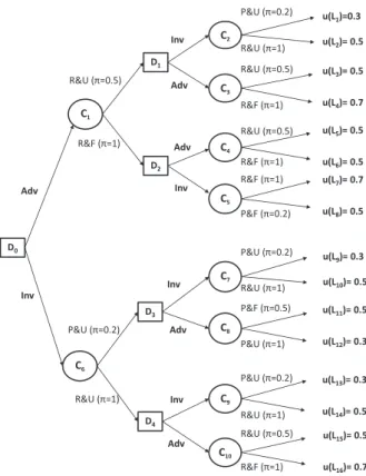
Example 1 Let us suppose that a “Rich and Unknown” person runs a startup company. In every state she must choose between Invest-ing (Inv) or AdvertisInvest-ing (Adv) and she may be then Rich (R) or Poor (P) and Famous (F) or Unknown (U). Figure 1 shows the possibilis-tic decision tree (with horizonh = 2) that represents this decision problem. This tree has 8 strategies, 16 trajectories:
τ1 = (Adv, R&U, Inv, P &U ), τ2 = (Adv, R&U, Inv, R&U ),
τ3 = (Adv, R&U, Adv, R&U ), τ4 = (Adv, R&U, Adv, R&F ),
τ5 = (Adv, R&F, Adv, R&U ), τ6 = (Adv, R&F, Adv, R&F ),
etc.
The evaluation of a possibilistic strategy, as proposed by [22], relies on the qualitative optimistic and pessimistic decision criteria axiom-atized by [11]. The utility of the strategy is computed on the basis of the transition possibilities and the utilities of its trajectories. For each trajectory τ = (aj0, xi1, aj1, . . . , xih):
6 As in classical probabilistic decision trees, it is assumed that π(X j =
x|past(Cj)) only depends on the variables in past(Cj) and actually only
on the decision made in the preceding node and on the state of the preceding chance node. u(L3)= 0.5 u(L4)= 0.7 C2 D2 u(L1)=0.3 u(L2)= 0.5 D1 D0 C1 Adv Inv Adv Inv C3 R&U (π=0.5) R&F (π=1) R&F (π=1) R&U (π=0.5) P&U (π=0.2) R&U (π=1) u(L11)= 0.5 u(L12)= 0.3 C7 C9 D4 u(L9)= 0.3 u(L10)= 0.5 D3 C6 Adv Inv Inv C8 P&U (π=0.2) R&U (π=1) P&U (π=1) P&F (π=0.5) P&U (π=0.2) R&U (π=1) R&U (π=1) P&U (π=0.2) u(L13)= 0.3 u(L14)= 0.5 C10 Adv R&F (π=1) R&U (π=0.5) u(L15)= 0.5 u(L16)= 0.7 C4 Adv R&F (π=1) R&U (π=0.5) C5 P&F (π=0.2) R&F (π=1) u(L7)= 0.7 u(L8)= 0.5 Inv u(L5)= 0.5 u(L6)= 0.5
Figure 1. The possibilistic decision tree of Example 1
• Its utility denoted u(τ ), is the utility u(xih) of its leaf.
• The possibility of τ given that a strategy δ is applied from initial
node D0is defined by:
π(τ |δ, D0) = (
min
k=1..hπjk−1(xik) if τ is a trajectory of δ,
0 otherwise.
where πjk−1is the possibility distribution at Cjk−1.
It is now possible to compute, for any δ ∈ ∆ its optimistic and
pessimistic utility degrees (the higher, the better):
uopt(δ) = max
τ∈δ min(π(τ |δ, D0), u(τ ))
upes(δ) = min
τ∈δmax (1 − π(τ |δ, D0), u(τ ))
This approach is purely ordinal (only min and max operations are used to aggregate the evaluations of the possibility of events and the ones of the utility of states). We can check that the preference
order-ings+Obetween strategies, derived either from uopt(O= uopt) or
from upes(O= upes), satisfy the principle of weak monotonicity:
∀Cj∈ NCj,∀Di∈ Succ(Cj), δ, δ
′∈ ∆
Di, δ” ∈ ∆Succ(Cj)\Di:
δ+Oδ′ =⇒ δ + δ” +Oδ′+ δ′′
This property guarantees that dynamic programming [2] applies, and provides an optimal strategy in time polynomial with the size of the tree: [21, 22] have proposed qualitative counterparts of stochastic dy-namic programming algorithms: in the finite horizon case backwards induction, or in the infinite horizon case value and policy iteration.
The basic pessimistic and optimistic utilities nevertheless present a severe drawback, known as the ”drowning effect”, due to the use of idempotent operations. In particular, when two strategies give an
identical and extreme (either good, for uoptor bad, for upes), utility
in some plausible trajectory, they may be undistinguished although they may give significantly different consequences in other possible trajectories, as illustrated in Example 2.
Example 2 Let δ and δ′ be the two strategies of Example 1
de-fined by δ(D0) = δ′(D0) = Adv; δ(D1) = Inv; δ′(D1) = Adv; δ(D2) = δ′(D2) = Adv. δ gathers 4 trajectories, τ1, τ2, τ5, τ6withπ(τ1|D0, δ) = 0.2 and u(τ1) = 0.3; π(τ2|D0, δ) = 0.5 and
u(τ2) = 0.5 ; π(τ5|D0, δ) = 0.5 and u(τ5) = 0.5; π(τ6|D0, δ) =
1 and u(τ5) = 0.5. Hence uopt(δ) = upes(δ) = 0.5.
- δ′ is also composed of 4 trajectories (τ
3, τ4, τ5, τ6). Hence uopt(δ′) = upes(δ′) = 0.5.
Thusuopt(δ) = uopt(δ′) and upes(δ) = upes(δ′): δ′, which pro-vides at least utility0.5 in all trajectories, is not preferred to δ that provides a bad utility (0.3) in some non impossible trajectory (τ1).τ2, which is good and totally possible ”drowns” the bad consequence of
δ in τ1in the optimistic comparison; in the pessimistic one, the bad
utility ofτ1is drowned by its low possibility, hence a global degree upesthat is equal to the one ofδ′(that, once again, guarantees a0.5 utility degree at least).
The two possibilistic criteria thus may fail to satisfy the principle of Pareto efficiency, that may be written as follows, for any optimiza-tion criterion O (here upesor uopt):
∀δ, δ′ ∈ ∆, if (i) ∀D ∈ Common(δ, δ′), δ
D +O δ′D and (ii)
∃D ∈ Common(δD, δD′ ), δD≻OδD′ , then δ≻Oδ′
where Common(δ, δ′) is the set of nodes for which both δ and δ′
provide an action and δD(resp. δD′ ) is the restriction of δ (resp. δ′) to the subtree rooted in D.
Moreover, neither uoptor upesdo fully satisfy the classical, strict,
monotonicity principle, that can be written as follows:
∀Cj ∈ NC, Di∈ Succ(Cj), δ, δ′∈ ∆Di, δ” ∈ ∆Succ(Cj)\Di,
δ+Oδ′ ⇐⇒ δ + δ” +Oδ′+ δ′′
It may indeed happen that upes(δ) > upes(δ′) while
upes(δ + δ”) = upes(δ′+ δ”) (or that uopt(δ) > uopt(δ′) while
uopt(δ + δ”) = uopt(δ′+ δ”)).
The purpose of the present work is to build efficient preference relations that agree with the qualitative utilities when the latter can
make a decision, and break ties when not - to build refinements7
that satisfy the principle of Pareto efficiency.
3
Escaping the drowning effect by leximin and
leximax comparisons
The possibilistic drowning effect is due to the use ofmin and max
operations. In ordinal aggregations, this drawback is well known and it has been overcome by means of leximin and leximax comparisons
[17]. More formally, for any two vectors t and t′:
• t +lmint′iff∀i, tσ(i)= t′σ(i)or∃i∗,∀i < i∗, tσ(i)= t′σ(i)and tσ(i∗)> t′σ(i∗)
• t +lmaxt′iff∀i, tµ(i)= t′µ(i)or∃i∗,∀i < i∗, tµ(i)= t′µ(i)and tµ(i∗)> t′µ(i∗)
7Formally, a preference relation!′refines a preference relation! if and
only if whatever δ, δ′, if δ≻ δ′then δ≻′δ′.
where, for any vector v (here, v= t or v = t′), v
µ(i)(resp. vσ(i))
is the ithbest (resp. worst) element of v.
The refinements of uoptand upesby lexicographic principles have
been considered by [13] for non sequential problems; in this context, a decision is a possibility distribution π over the utility degrees, i.e.
a vector of pairs(π(u), u). Then it is possible to write:
• π Dlmax(lmin) π′ iff∀i, (π(u), u)µ(i) ∼lmin (π′(u), u)µ(i)or
∃i∗,∀i < i∗, (π(u), u)
µ(i)∼lmin(π′(u), u)µ(i)and
(π(u), u)µ(i∗)≻lmin(π′(u), u)µ(i∗).
• π Dlmin(lmax) π′ iff ∀i, (1 − π(u), u)σ(i) ∼lmax (1 −
π′(u), u)
σ(i) or∃i∗,∀i < i∗, (1 − π(u), u)σ(i) ∼lmax (1 −
π′(u), u)
σ(i)and(1 − π(u), u)σ(i∗)≻lmax(1 − π′(u), u)µ(i∗).
where(π(u), u)µ(i)is the ithbest pair of(π(u), u) according to
lmin and(1 − π(u), u)σ(i)is the ithworst pair of(1 − π(u), u)
according to lmax.
A straightforward way of applying this to sequential decision is to reduce the compound possibility distribution corresponding to the strategy, as usually done in possibilistic (and probabilistic) decision
trees. The reduction of δ yields the distribution πδon the utility
de-grees, defined by: πδ(u) = max
τ,u(τ )=uπ(τ |δ, D0). Then we can write: δ Dlmax(lmin)δ′ iff πδDlmax(lmin)πδ′,
δ Dlmin(lmax)δ′ iff πδDlmin(lmax)πδ′.
Dlmax(lmin)(resp. Dlmin(lmax)) refines+uopt(resp.+upes), but
neither Dlmax(lmin)nor Dlmin(lmax)do satisfy Pareto efficiency, as
shown by the following counterexample.
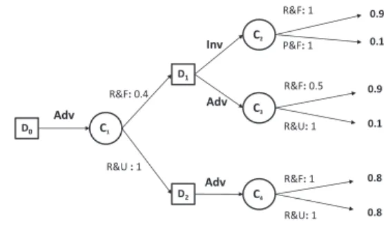
Example 3 Consider a modified version of the problem of Example 1 (Figure 2).δ and δ′ are the two strategies defined by:δ(D0) =
δ′(D0) = Adv, δ(D1) = Inv, δ′ = (D1) = Adv, δ(D2) =
δD′2 = Adv. Common(δ, δ ′) = {D 0, D1, D2}, δD0 = δ ′ D0, δD2 = δ ′ D2 and δD1 dominates δ ′ D1 w.r.t. lmax(lmin), since
((1, 0.1), (1, 0.9)) ⊲lmax(lmin)((1, 0.1)(0.5, 0.9)). δ should then be
strictly preferred toδ′. By reduction, we getπ
δ(0.9) = πδ(0.1) =
min(0.4, 1) = 0.4 and πδ(0.8) = min(1, 1) = 1 and for δ′we have
πδ′(0.9) = min(0.4, 0.5) = 0.4, πδ′(0.1) = min(0.4, 1) = 0.4
and πδ′(0.8) = min(1, 1) = 1: δ and δ′ are indifferent for
Dlmax(lmin). This contradicts Pareto efficiency.
Inv Adv 0.9 0.1 C2 C4 D2 0.9 0.1 D1 D0 C1 C3 R&F: 0.4 R&U : 1 R&U: 1 R&F: 0.5 R&F: 1 P&F: 1 R&U: 1 R&F: 1 0.8 0.8 Adv Adv
Figure 2. A counter example at the efficiency of Dlmax(lmin)
The drowning effect at work here is due to the reduction of strategies, namely to the fact that the possibility of a trajectory
is drowned by the one of the least possible of its edges. That is why we propose to give up the principle of reduction and to build lexicographic comparisons on strategies considered in extenso.
Recall that: uopt(δ) = max
τ∈δ min ! min k=1..hπjk−1(xik); u(xih) " .
Then, for any τ = (aj0, xi1, . . . , ajh−1, xih) and τ
′ =
(aj′
0, xi′1, . . . , aj′h−1, xi′h), we define +lminand+lmaxby: • τ +lmin τ′ iff (πj0(xi1), . . . , πjh−1(xih), u(xih)) +lmin
(πj′
0(xi′1), . . . , πjh−1′ (xi′h), u(xi′h))
• τ +lmax τ′ iff (1 − πj0(xi1), . . . , 1 − πjh−1(xih), u(xih)) +lmax(1 − πj′
0(xi′1), . . . , 1 − πj′h−1(xi′h), u(xi′h))
Hence the proposition of the following preference relations8:
• δ +lmax(lmin) δ′ iff ∀i, τµ(i) ∼lmin τµ(i)′ or ∃i∗,∀i ≤
i∗, τµ(i)∼lminτµ(i)′ and τµ(i∗)≻lminτµ(i′ ∗),
• δ +lmin(lmax) δ′iff∀i, τσ(i) ∼lmax τσ(i)′ or∀i, τσ(i) ∼lmax
τσ(i)′ or∃i∗,∀i ≤ i∗, τ
σ(i)∼lmaxτσ(i)′ and τσ(i∗)≻lmaxτσ(i′ ∗), where τµ(i) (resp. τµ(i)′ ) is the i
th
best trajectory of δ (resp δ′) ac-cording to+lminand τσ(i)(resp. τσ(i)′ ) is the ithworst trajectory of
δ (resp δ′) according to+
lmax.
These relations are relevant refinements and escape the drowning effect - they are those we are looking for:
Proposition 1 +lmax(lmin) is complete, transitive and refines
+uopt;+lmin(lmax)is complete, transitive and refines+upes.
Proposition 2 +lmax(lmin)and+lmin(lmax)both satisfy the
prin-ciple of Pareto efficiency as well as strict monotonicity.
Propositions 1 and 2 have important consequences; from a pre-scriptive point of view, they outline the rationality of lmax(lmin) and lmin(lmax) and suggest a probabilistic interpretation, which we develop in Section 5. From a practical point of view, they allow us to define a dynamic programming algorithm to get lexi optimal solutions - this is the topic of the next Section.
4
Dynamic Programming for lexi qualitative
criteria
The algorithm we propose (Algorithm 1 for the lmax(lmin) variant; the lmin(lmax) variant is similar) proceeds in the classical way, by backwards induction: when a chance node is reached, an optimal sub-strategy is recursively built for each of its children; these substrate-gies are combined but the resulting strategy is NOT reduced, contrar-ily to what is classically done; when a decision node is reached, the program is called for each child and the best of them is selected.
The comparison of strategies is done on the basis of the matrices of their trajectories (denoted ρ ; each line gathers the possibility and utility degrees of a trajectory τ= (aj0, xi1, aj1, . . . , ajh, xih)):
ρlt= πjt−1&xit ' if t≤ h, O = lmax&lmin' 1 − πjt−1&xit ' if t≤ h, O = lmin&lmax' u&xih ' if t= h + 1.
So as to allow fast comparisons, the matrices are built incrementally and ordered on the fly by the function ConcatAndOrder: when a 8If the strategies have different numbers of trajectories, neutral trajectories
(vectors) are added to the shortest strategy, at the bottom of the shortest list of trajectories
Algorithm 1: DynProgLmaxLmin(N :Node)
Data: δ, the strategy built by the algorithm, is a global variable
Result: Computes δ forDTNand returns the maxtrix of its
trajectories, ρ begin // Leaves ifN∈ NUthenρ= [u(N )]; // Chance nodes ifN∈ C then k= |Succ(N )|; forDi∈ Succ(N ) do ρi← DynP rogLmaxLmin(Di); ρ← ConcatAndOrder(ρ1, . . . , ρk, πN); // Decision nodes ifN∈ D then ρ← [0] foreachaj∈ Out(N ) do ρj ← DynP rogLmaxLmin(Succ(N, aj)); ifρj +lmax(lmin)ρ then ρ← ρj and δ(N ) ← aj; returnρ;
chance node, say Cj is reached, k = |Succ(Cj)| substrategies are
built recursively and their matrices ρ1, . . . , ρkare computed. Matrix
ρ of the current (compound) strategy, for the subtree rooted in Cj,
is obtained by calling ConcatAndOrder&ρ1, . . . , ρk, πCj'. This
function adds a column to each ρi, filled with πj(xi) ; the matrices
are vertically concatenated; then the elements in the lines are ordered in decreasing (resp. increasing) order, and the lines are reordered by decreasing (resp. increasing) order w.r.t. to lmax (resp. lmin). As
a matter of fact, once ρ has been reordered, ρ1,1is always equal to
uopt(δ) (resp. upes(δ)).
The lexicographic comparison of two strategies δ and δ′ is
per-formed by scanning the elements ρl,tand ρ′l,tof ρ and ρ′in parallel, line by line from the first one. The first pair of different(ρl,t, ρ′l,t) de-termines the best matrix/strategy. If the matrices have different num-bers of lines, neutral lines are added at the bottom of the shortest one
(filled with0 for the optimistic case, with 1 for the pessimistic one).
Even if working with matrices rather than numerical values, the algorithm is polynomial w.r.t. the size of the original tree. This is because (i) the algorithm crosses each edge of the tree only once (as in the classical version), (ii) the matrices are never bigger than the strategies and (iii) the comparison of strategies is done in time linear with their size - thus linear with the size of the original tree.
5
Lexi comparisons and Expected Utility
If the problem is not sequential, it is easy to see that the comparison
of possibilistic utility distributions by+lmax(lmin)and+lmin(lmax)
do satisfy the axioms of EU. [13] have indeed shown that these deci-sion criteria can be captured by an EU - namely, relying on infinites-imal probabilities and utilities. In this Section, we claim that such a result can be extended to sequential problems - for decision trees.
The proof relies on a transformation of the possibilistic tree into a probabilistic one. The graphical components are identical and so are the sets of admissible strategies. In the optimistic case the prob-ability and utility distributions are chosen in such a way that the lmax(lmin) and EU criteria do provide the same preference on ∆.
that maps each possibility distribution to an additive distribution and each utility level into an additive one; this transformation is required to satisfy the following condition:
(R) : ∀α, α′∈ L such that α > α′: φ(α)h+1> bh
φ(α′), where b is the branching factor of the tree. Condition (R) guarantees that if uopt(δ) = α > uopt(δ′) = α′, then a comparison based on a sum-product approach on the new tree will also decide in favor of δ.
For any chance node Cj, a local transformation φjis then derived
from φ, such that φj satisfies both condition (R) and the
normaliza-tion condinormaliza-tion of probability theory. EUopt denotes the preference
relation provided by the EU-criterion on the probabilistic tree
ob-tained by replacing each πjby φj◦ πjand the utility function u by
φ◦ u. We show that:
Proposition 3 If (R) holds, then+EUoptrefines+uopt.
Proposition 4 δ+lmax(lmin)δ′iffδ+EUoptδ
′,∀(δ, δ′) ∈ ∆.
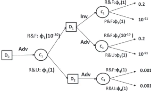
Example 4 φ(1) = 1, φ(0.9) = 0.2, φ(0.8) = 0.001, φ(0.5) =
10−10, φ(0.4) = 10−30, φ(0.1) = 10−91.
It holds thatφ(α)3 > φ(α′) ∗ 22, for allα > α′. We ob-tain the transformed conditional distributions by normalizing on each node. For instance for nodeC1,φ1(10−30) = 10
−30 1+10−30 and φ1(1) = 1+101−30, for nodeC2,φ2(1) = 1 1+1andφ2(1) = 0.5, for nodeC3,φ3(10−10) = 10 −10 1+10−10 andφ3(1) = 1 1+10−10, for node C4,φ4(1) = 0.5 and φ4(1) = 0.5. Adv a1 R&F:φ2(1) P&F:φ2(1) Inv Adv R&F:φ4(1) R&U:φ4(1) R&F:φ3(10-10 ) R&U:φ3(1) 0.2 10-91 R&F: φ1(10-30) R&U: φ1(1) D0 C1 C2 C3 C4 D1 D2 0.2 10-91 0.001 0.001 Adv
Figure 3. Transformed probabilistic decision tree of possibilisic decision tree of (counter)-example 3
The construction is a little more complex if we consider the +lmin(lmax)comparison, where the utility degrees are not directly
compared to possibility degrees π but to degrees1 − π. Hopefully,
it is possible to rely on the results obtained for the optimistic case, since the optimistic and pessimistic utilities are dual of each other.
Proposition 5 LetDTinv
the tree obtained fromDT by using util-ity functionu′ = 1 − u on leaves. It holds that: u
pes,DT(δ) ≥ upes,DT(δ′) iff uopt,DTinv(δ′) ≥ uopt,DTinv(δ)
As a consequence, we build an EU-based equivalent of +lmin(lmax), denoted+EUpes, by replacing each possibility
distri-bution πiinDT by the probability distribution φi◦ πi, as for the
optimistic case and each utility degree u byφ(1) − φ(u). It is then possible to show that:
Proposition 6 δ+lmin(lmax)δ′iffδ+EUpes δ
′,∀(δ, δ′) ∈ ∆. Propositions 4 and 6 show that lexi-comparisons have a proba-bilistic interpretation - actually, using infinitesimal probabilities and utilities. This result comforts the idea, first proposed by [4] and then by [13], of a bridge between qualitative approaches and probabilities, through the notion of big stepped probabilities [4, 24]. We make here a step further, by the identification of transformations that support sequential decision making.
Beyond this theoretical argument, this result suggests an al-ternative algorithm for the optimization of lmax(lmin) (resp. lmin(lmax)): simply transform the possibilistic decision tree into a probabilistic one and use a classical, EU-based algorithm of dy-namic programming. In a perfect world, both approaches solve the problem in the same way and provide the same optimal strategies -the difference being that -the first one is based on -the comparison of
matrices, the second one on expected utilities in R+. The point is
that the latter handles infinitesimals; then either the program is based on an explicit handling of infinitesimals, and proceeds just like the matrix-based comparison, or it lets the programming language han-dle these numbers in its own way - and, given the precision of the computation, provides approximations.
6
Experiments
We thus get three criteria for each of the pessimistic and optimistic approaches: the basic possibilistic ones, the lexicographic refine-ments described in Section 3, and the EU approximations of the
lat-ter. We compare the3 variants within each series with two measures:
the CPU time and a pairwise success rate: SuccessA
B is the
per-centage of solutions provided by an algorithm optimizing criterion A that are optimal with respect to criterion B; for instance, the lower
Success uopt
lmax(lmin), the more important the drowning effect.
The backward induction algorithms corresponding to the six crite-ria have been implemented in Java. As to the EU-based approaches, the transformation function depends on the horizon h and the
branch-ing factor b (here b= 2). We used φ(1L) = 1, φ(αi) =φ(αi+1)
h+1
bh∗1.1 ,
each φj being obtained by normalization of φ on Cj. The
experi-ments have been performed on an Intel Core i5 processor computer (1.70 GHz) with 8GB DDR3L of RAM..
The tests were performed on complete binary decision trees,
for h = 2 to h = 7, that are randomly generated. The first
node is a decision node: at each decision level from the root
(i = 1) to the last level (i = 7) the tree contains 2i−1
deci-sion nodes.This means that with h = 2 (resp. 3, 4, 5, 6, 7), the
number of decision nodes is equal to 5 (resp. 21, 85, 341, 1365,
5461) The utility values are uniformly randomly fired in the set
L = {0.1, 0.2, 0.3, 0.4, 0.5, 0.6, 0.7, 0.8, 0.9, 1}. Conditional
pos-sibilities relative to chance nodes are normalized, one edge having possibility one and the possibility degree of the other is uniformly
fired in L. For each value of h,100 decision trees are generated.
Figure 4 presents the average execution CPU time for the six crite-ria. We observe that, whatever the optimized criterion, the CPU time increases linearly w.r.t. the number of decision nodes, which is in line with what we could expect. Furthermore, it remains affordable
with big trees: the maximal CPU time is lower than1s for a
deci-sion tree with 5461 decideci-sion nodes. It appears that uopt is always
faster than EUopt, which is 1.5 or 2 times faster than lmax(lmin)
The same conclusion is drawn when comparing lmin(lmax) to upes
and EUpes. These results are easy to explain: (i) the manipulation of
(ii) the handling of numbers by min and max operations is faster than sum-product manipulations of infinitesimal.
0,2 1 5 25 125 625 3125 5 21 85 341 1365 5461
Average CPU time for the pessimistic criteria
upes EUpes lmin(lmax) CPU time in m s
Number of decision nodes 0,2 1 5 25 125 625 5 21 85 341 1365 5461
Average CPU time for the optimistic criteria
uopt EUopt lmax(lmin) CPU time in m s
Number of decision nodes
Figure 4. Average CPU time (in ms) for h=2 to 7
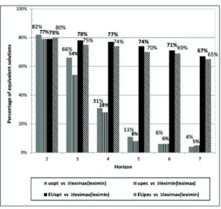
As to the success rate, the results are described in Figure 5. The percentage of solutions optimal for uopt(resp. for upes) that are also optimal for lmax(lmin) (resp. lmin(lmax)) is never more than 82%, and decreases when the horizon increases: the drowning ef-fect is not negligible and increases with the length of the trajectories. Moreover EUopt(resp. EUpes) does not perform well as an approx-imation of lmax(lmin) (resp. lmin(lmax)): the percentage of so-lutions optimal for the former which are also optimal for the latter is lower than80% in all cases, and decreases when h increases. This is easily explained by the fact that the probabilities are infinitesimals and converge to0 when the length of the branches (and thus the num-ber of factors in the products) increase, as suggested in Section 5.
These experiments conclude in favor of the lexi refinements in their full definition - their approximation by expected utilities are comparable in terms of CPU efficiency but not precise enough. The EU criteria nevertheless offer a better approximation than uoptand upeswhen space is limited (or when h increases).
7
Concluding remarks
This work has both theoretical and practical implications. It extends and generalizes to sequential problems the theoretical links estab-lished in [13] between possibilistic utilities and expected utilities. It performs better that the refinement of binary possibilistic utilities
Figure 5. Sucess rate
(BPU) proposed in [27] for Binary Possibilistic Utilities and as a particular case, to classical, optimitic and pessimistic, possibilitistic utilities. In [27]’s treatment indeed, two similar trajectories of the same strategy are merged. The resulting criterion thus suffers from a drowning effect and does no satisfy strict monotonicity: as such, it cannot be represented by an EU-based criterion which “counts” trajectories (weighted by their probabilities). We actually do refine [27]’s criterion. Incorporating our lexicographic refinements in BPU would lead to a more powerful refinement and suggests a probabilis-tic interpretation of efficient BPU. It also leads to new planning al-gorithms that are more “decisive” than their original counterparts.
The perspectives of our work are twofold. First, our approach could be naturally extended to solve possibilistic Markov Decision Processes.This extension seems theoretically straightforward, since a finite-horizon MDP can be translated into a set of decision trees (one for each state). Thus, our theoretical results hold for finite-horizon MDPs as well. However, the direct application of the lexicographic approach to possibilistic MDPs may lead to algorithms which are exponential in time and space (w.r.t. the MDP description), since the decision trees associated to a MDP may be of exponential size, while (possibilistic) MDPs can be solved in polynomial time [22, 21]. De-termining whether computing lexicographic optimal solutions to pos-sibilistic MDPs is tractable is a perspective of this work.
The second perspective of this work, not unrelated, is to develop simulation-based algorithms for finding lexicographic solutions to MDPs. Reinforcement Learning algorithms [26] allow to solve large size MDPs by making use of simulated trajectories of states to opti-mize a strategy. It is not immediate to develop RL algorithms for pos-sibilistic MDPs, since no unique stochastic transition function corre-sponds to a possibility distribution. However, uniform simulation of trajectories (with random choice of actions) may be used to gener-ate an approximation of the possibilistic decision tree (provided that both transition possibilities and utility of the leaf are given with the simulated trajectory). So, interleaving simulations and lexicographic dynamic programming may lead to RL-type algorithms for approxi-mating lexicographic-optimal policies for (large) possibilistic MDPs.
REFERENCES
[1] Kim Bauters, Weiru Liu, and Llu’is Godo, ‘Anytime algorithms for solving possibilistic MDPs and hybrid MDPs’, in 9th International
Symposium on Foundations of Information and Knowledge Systems (FoIKS’16), eds., Marc Gyssens and Guillermo Simari, Lecture Notes in Artificial Intelligence, pp. 1–18. Springer International Publishing Switzerland, (2016).
[2] Richard Bellman, Dynamic Programming, Princeton University Press, 1957.
[3] Nahla Ben Amor, H´el`ene Fargier, and Wided Guezguez, ‘Possibilis-tic sequential decision making’, International Journal of Approximate
Reasoning, 55, 1269–1300, (2014).
[4] Salem Benferhat, Didier Dubois, and Henri Prade, ‘Possibilistic and standard probabilistic semantics of conditional knowledge bases’,
Jour-nal of Logic and Computation, 9, 873–895, (1999).
[5] Blai Bonet and Hector Geffner, ‘Arguing for decisions: A qualitative model of decision making’, in 12th Conference on Uncertainty in
Ar-tificial Intelligence (UAI-96), August 1-4, Portland, Oregon, USA, pp. 98–105, (1996).
[6] Anthony R. Cassandra, Leslie Pack Kaelbling, and Michael L. Littman, ‘Acting optimally in partially observable stochastic domains’, in 12th
National Conference on Artificial Intelligence (AAAI’13), July 31 - Au-gust 4 Seattle, WA, USA, pp. 1023–1028, (1994).
[7] Francis C. Chu and Joseph Y. Halpern, ‘Great expectations. part I: on the customizability of generalized expected utility’, in 18th
Interna-tional Joint Conference on Artificial Intelligence (IJCAI-03), August 9-15,2013, Acapulco, Mexico, pp. 291–296, (2003).
[8] Nicolas Drougard, Florent Teichteil-Konigsbuch, Jean-Loup Farges, and Didier Dubois, ‘Qualitative possibilistic mixed-observable MDPs’, in 29th Conference on Uncertainty in Artificial Intelligence (UAI’13),
August 11-15,2013, Bellevue, WA, USA, pp. 192–201, (2013). [9] Nicolas Drougard, Florent Teichteil-Konigsbuch, Jean-Loup Farges,
and Didier Dubois, ‘Structured possibilistic planning using decision di-agrams’, in 28th Conference on Artificial Intelligence (AAAI’14), July
27 -31, 2014, Qu´ebec City, Qu´ebec, Canada., pp. 2257–2263, (2014). [10] Didier Dubois, Lluis Godo, Henri Prade, and Adriana Zapico,
‘Mak-ing decision in a qualitative sett‘Mak-ing: from decision under uncertainty to case-based decision’, in 6th International Conference on Principles of
Knowledge Representation and Reasoning (KR’98), June 2-5, Trento, Italy, pp. 594–605, (1998).
[11] Didier Dubois and Henri Prade, ‘Possibility theory as a basis for quali-tative decision theory’, in 14th international joint conference on
Artifi-cial intelligence (IJCAI’95), August 20-25, Montreal, Quebec Canada, pp. 1925–1930, (1995).
[12] Didier Dubois, Henri Prade, and R´egis Sabbadin, ‘Decision-theoretic foundations of qualitative possibility theory’, European Journal of
Op-erational Research, 128, 459–478, (2001).
[13] H´el`ene Fargier and R´egis Sabbadin, ‘Qualitative decision under uncer-tainty: back to expected utility’, Artificial Intelligence, 164, 245–280, (2005).
[14] Phan Giang and Prakash P Shenoy, ‘Two axiomatic approaches to deci-sion making using possibility theory’, European Journal of Operational
Research, 162, 450–467, (2005).
[15] Lluis Godo and Adriana Zapico, ‘On the possibilistic-based decision model: Characterization of preference relations under partial inconsis-tency’, Applied Intelligence, 14, 319–333, (2001).
[16] Daniel J. Lehmann, ‘Generalized qualitative probability: Savage revis-ited.’, in 21st Conference in Uncertainty in Artificial Intelligence (UAI
’05), July 26-29, Edinburgh, Scotland, pp. 381–388, (1996). [17] Hervi Moulin, Axioms of Cooperative Decision Making, Cambridge
University Press, 1988.
[18] John Von Neumann and Oskar Morgenstern, Theory of games and
eco-nomic behavior, 1948.
[19] Martin L. Puterman, Markov Decision Processes, John Wiley and Sons, 1994.
[20] Howard Raiffa, Decision Analysis: Introductory Lectures on Choices
under Uncertainty, Addison Wesley, 1968.
[21] R´egis. Sabbadin, ‘Possibilistic Markov decision processes’,
Engineer-ing Applications of Artificial Intelligence, 14, 287–300, (2001). [22] R´egis Sabbadin, H´el`ene Fargier, and J´rome Lang, ‘Towards qualitative
approaches to multi-stage decision making’, International Journal of
Approximate Reasoning, 19, 441–471, (1998).
[23] Leonard J. Savage, The Foundations of Statistics, Wiley, 1954.
[24] Paul Snow, ‘Diverse confidence levels in a probabilistic semantics for conditional logics’, Artificial Intelligence, 113, 269–279, (1999). [25] Richard S. Sutton, ‘Learning to predict by the methods of temporal
differences’, in Machine Learning, pp. 9–44, (1988).
[26] Richard S. Sutton and Andrew G. Barto, Reinforcement Learning:An
Introduction, MIT Press, 1998.
[27] Paul Weng, ‘Qualitative decision making under possibilistic uncer-tainty: Toward more discriminating criteria’, in 21st Conference in
Uncertainty in Artificial Intelligence (UAI’05), July 26-29, Edinburgh, Scotland, pp. 615–622, (2005).
[28] Paul Weng, ‘Axiomatic foundations for a class of generalized expected utility: Algebraic expected utility’, in 22nd Conference Annual
Con-ference on Uncertainty in Artificial Intelligence (UAI-06), July 13-16 , Arlington, Virginia, pp. 520–527, (2006).