Implementation of a coupled computational chain to the combustion chamber's heat transfer

En vue de l'obtention du

DOCTORAT DE L'UNIVERSITÉ DE TOULOUSE

Délivré par :

Institut National Polytechnique de Toulouse (INP Toulouse)

Discipline ou spécialité :

Energétique et Transferts

Présentée et soutenue par :

Mme SANDRINE BERGER

le lundi 20 juin 2016

Titre :

Unité de recherche :

Ecole doctorale :

MISE EN OEUVRE D'UNE CHAINE DE CALCUL COUPLE POUR LA

THERMIQUE DE CHAMBRE DE COMBUSTION

Mécanique, Energétique, Génie civil, Procédés (MEGeP)

Centre Européen de Recherche et Formation Avancées en Calcul Scientifique (CERFACS)

Directeur(s) de Thèse :

M. LAURENT GICQUEL M. FLORENT DUCHAINE

Rapporteurs :

Mme DANIELE ESCUDIE, INSA LYON M. OLIVIER GICQUEL, ECOLE CENTRALE PARIS

Membre(s) du jury :

1 Mme DANIELE ESCUDIE, INSA LYON, Président

2 M. FLORENT DUCHAINE, CERFACS, Membre

2 M. LAURENT GICQUEL, CERFACS, Membre

2 M. MARC-PAUL ERRERA, ONERA, Membre

R´

esum´

e

La conception des moteurs a´eronautiques est soumise `a de nombreuses contraintes telles que les gains de performance ou les normes environnementales de plus en plus exigeantes. Face `a ces objectifs souvent contradictoires, les nouvelles technologies de moteur tendent vers une augmen-tation de la temp´erature locale et globale dans les ´etages chauds. En cons´equence, les parties solides comme les parois du brˆuleur sont soumises `a des niveaux de temp´erature ´elev´es ainsi que d’importants gradients de temp´erature, tous deux critiques pour la dur´ee de vie du moteur. Il est donc essentiel pour les concepteurs de caract´eriser pr´ecis´ement la thermique locale de ces syst`emes. Aujourd’hui, la temp´erature de paroi est ´evalu´ee par des essais de coloration. Pour limiter ces essais relativement chers et complexes, des outils num´eriques haute fid´elit´e capables de pr´edire la temp´erature de paroi des chambres de combustion sont actuellement d´evelopp´es. Cet exercice n´ecessite de consid´erer tous les modes de transfert de chaleur (convection, conduction et rayon-nement) ainsi que la combustion au sein du brˆuleur. Ce probl`eme multi-physique peut ˆetre r´esolu num´eriquement `a l’aide de diff´erentes approches num´eriques. La m´ethode utilis´ee dans ce travail repose sur une approche partitionn´ee qui inclut la r´esolution de l’´ecoulement turbulent r´eactif par un code de simulation aux grandes ´echelles (LES), un solveur radiatif bas´e sur la m´ethode aux ordonn´ees discr`etes ainsi qu’un code de conduction solide. Les diverses questions et difficult´es li´ees `a la r´epartition des ressources informatiques ainsi qu’`a la m´ethodologie de couplage employ´ee pour traiter les disparit´es d’´echelles de temps et d’espace pr´esentes dans chacun des modes de transfert de chaleur sont discut´ees. La performance informatique des applications coupl´ees est ´etudi´ee `a travers un mod`ele tr`es simplifi´e ainsi que sur une application industrielle. Les param`etres impor-tants sont identifi´es et des pistes potentielles d’am´elioration sont propos´ees. La m´ethodologie de couplage thermique est ensuite ´etudi´ee du point de vue physique sur deux configurations distinctes. Pour commencer, l’´equilibre thermique entre un fluide r´eactif et un solide est ´etudi´e pour une con-figuration acad´emique d’accroche flamme. L’influence de la temp´erature de paroi de l’accroche flamme sur la stabilisation de flamme est mise en ´evidence sur des simulations fluide-seul. Ces r´esultats indiquent trois ´etats d’´equilibre th´eorique diff´erents. La pertinence physique de ces trois ´etats est ensuite ´evalu´ee `a l’aide de diverses simulations de transfert de chaleur conjugu´e r´ealis´ees pour diff´erentes solutions initiales et conductivit´es solides. Les r´esultats indiquent que seulement deux ´etats d’´equilibre ont un sens physique et que la bifurcation entre les deux ´etats possibles d´epend `a la fois de la condition initiale et de la conductivit´e solide. De plus, pour la gamme de

chapter 0.

param`etres test´es, la m´ethodologie de couplage n’a pas d’effet sur les solutions obtenues. Une m´ethodologie similaire est ensuite appliqu´ee `a une chambre de combustion d’h´elicopt`ere pour laquelle le rayonnement est de plus pris en compte. Diverses simulations sont pr´esent´ees afin d’´evaluer l’impact de chacun des processus de transfert de chaleur sur le champ de temp´erature : une simulation fluide-seul adiabatique de r´ef´erence, de transfert de chaleur conjugu´e, d’interaction thermique fluide-rayonnement ainsi qu’une simulation incluant toutes les physiques. Ces calculs montrent la faisabilit´e d’un couplage LES/conduction solide dans un contexte industriel et four-nissent de bonnes tendances de distribution de temp´erature. Pour finir, pour cette g´eom´etrie de brˆuleur et la condition d’op´eration simul´ee, les divers r´esultats montrent que le rayonnement joue un rˆole important dans la distribution des temp´eratures de paroi. De ce fait, les comparaisons aux essais de coloration sont globalement en meilleur accord quand les trois modes de transfert sont pris en compte.

Abstract

The design of aeronautical engines is subject to many constraints that cover performance gain as well as increasingly sensitive environmental issues. These often contradicting objectives are cur-rently being answered through an increase in the local and global temperature in the hot stages of the engine. As a result, the solid parts encounter very high temperature levels and gradients that are critical for the engine lifespan. Combustion chamber walls in particular are subject to large thermal constraints. It is thus essential for designers to characterize accurately the local thermal state of such devices. Today, wall temperature evaluation is obtained experimentally by complex thermocolor tests. To limit such expensive experiments, efforts are currently performed to provide high fidelity numerical tools able to predict the combustion chamber wall temperature. This spe-cific thermal field however requires the consideration of all the modes of heat transfer (convection, conduction and radiation) and the heat production (through the chemical reaction) within the burner. The resolution of such a multi-physic problem can be done numerically through the use of several dedicated numerical and algorithmic approaches. In this manuscript, the methodology relies on a partitioned coupling approach, based on a Large Eddy Simulation (LES) solver to resolve the flow motion and the chemical reactions, a Discrete Ordinate Method (DOM) radiation solver and an unsteady solid conduction code. The various issues related to computer resources distribution as well as the coupling methodology employed to deal with disparity of time and space scales present in each mode of heat transfer are addressed in this manuscript. Coupled application high performance studies, carried out both on a toy model and an industrial burner configuration evidence parameters of importance as well as potential path of improvements. The thermal coupling approach is then considered from a physical point of view on two distinct con-figurations. First, one addresses the impact of the methodology and the thermal equilibrium state between a reacting fluid and a solid for a simple flame holder academic case. The effect of the flame holder wall temperature on the flame stabilization pattern is addressed through fluid-only predictions. These simulations highlight interestingly three different theoretical equilibrium states. The physical relevance of these three states is then assessed through the computation of several CHT simulations for different initial solutions and solid conductivities. It is shown that only two equilibrium states are physical and that bifurcation between the two possible physi-cal states depends both on solid conductivity and initial condition. Furthermore, the coupling methodology is shown to have no impact on the solutions within the range of parameters tested.

chapter 0.

A similar methodology is then applied to a helicopter combustor for which radiative heat transfer is additionally considered. Different computations are presented to assess the role of each heat transfer process on the temperature field: a reference adiabatic fluid-only simulation, Conjugate Heat Transfer, Radiation-Fluid Thermal Interaction and fully coupled simulations are performed. It is shown that coupling LES with conduction in walls is feasible in an industrial context with acceptable CPU costs and gives good trends of temperature repartition. Then, for the combustor geometry and operating point studied, computations illustrate that radiation plays an important role in the wall temperature distribution. Comparisons with thermocolor tests are globally in a better agreement when the three solvers are coupled.

Un voyage de mille lieues commence toujours par un premier pas. Lao-Tseu

A tous ceux qui de pr`es ou de loin m’ont amen´ee ici aujourd’hui, A mes amis, `a ma famille, `a Nicolas...

Acknowledgements

Ca y est j’y suis ! C’est la fin d’un beau projet et le d´ebut d’un tout autre autour du monde. Ces ann´ees de th`ese ont ´et´e tr`es riches et m’ont beaucoup appris, tant en termes scientifiques et techniques que sur un plan humain. Dans cette si belle aventure, beaucoup de personnes m’ont apport´e leur expertise, leur aide et leur soutien et je souhaite aujourd’hui leur dire un sinc`ere et grand merci.

Je remercie tout d’abord les membres du jury, Dany Escudi´e et Olivier Gicquel, rapporteurs, ainsi que Mouna El Hafi et Marc-Paul Errera, examinateurs, qui ont accept´e d’´evaluer ce travail et m’ont fourni mati`ere `a de nouvelles r´eflexions.

Je pense ensuite `a mes encadrants de laboratoire a qui je transmet mon immense gratitude, Lau-rent Gicquel et FloLau-rent Duchaine qui sont partie int´egrante de ce travail et qui ont su chacun `a leur mani`ere m’apprendre ´enorm´ement, m’orienter, me soutenir et me transmettre leur passion pour ce domaine de recherche (et pour les palettes allant du bleu au rouge en passant par le vert). Je remercie `a cette occasion Florent d’avoir su rester patient face aux heures que j’ai pass´e dans son bureau `a m’int´erroger sur le sens profond de la thermique et de la CFD. Un grand merci ensuite `a mes encadrants industriels `a TURBOMECA, Thomas Lederlin, encadrant des premi`eres heures et St´ephane Richard qui a pris la rel`eve et m’a tant expliqu´e sur les moteurs d’h´elicopt`ere et les divers enjeux de leur d´eveloppement et qui a su d´efendre mon petit carr´e. J’en profite pour remercier Jean Lamouroux, qui m’a aussi apport´e son support dans la difficile tˆache de compren-dre et de dompter le moteur dont on ne doit pas prononcer le nom.

J’aimerais aussi remercier l’ensemble des s´eniors combustion qui d´etiennent cette fabuleuse exp´erience et cette capacit´e de recul si pr´ecieux pour nous petits th´esards avides de conseils et de solutions. Mes remerciements tout particuliers vont `a B´en´edicte Cuenot qui m’a ouvert la porte de la com-munaut´e combustion et m’a conseill´e pour les questions de rayonnement, Antoine Dauptain, dont la cr´eativit´e et l’ing´eniosit´e m’ont toujours fascin´ee dans son d´eveloppement de nouveaux outils et repr´esentations des moteurs et qui a su r´epondre pr´esent `a tous mes ”au secours, je repr´esente ¸ca comment avec un sch´ema???”, ainsi qu’ `a Gabriel Staffelbach, mon magicien HPC, d´eveloppement

chapter 0.

et d´epannage en tout genre, devenu un ami pr´ecieux. Puisqu’on parle de d´epannage en tout genre, je tiens `a adresser un grand merci `a toute l’´equipe de l’administration, et en particulier `a Marie, Michelle et Chantal (je crois que je n’ai jamais rencontr´e quelqu’un qui souriait autant) sans qui tout serait tellement plus compliqu´e. Mes remerciements aussi `a toute l’´equipe CSG qui rend tout ¸ca possible et garde le sourire quand on arrive avec toujours plus de questions, de demandes complexes et de probl`emes.

Mes remerciements vont aussi aux stagiaires, th´esards et post-docs de l’´equipe qui ont contribu´e `a faire de cette exp´erience une richesse. J’ai une pens´ee particuli`ere pour mes co-bureaux successifs, Damien, qui m’a si gentiment accueillie au labo et dans son monde et avec qui j’ai partag´e telle-ment de conversations passionnantes et passionn´ees et de tranches de vie, Nikos, co-bureau des derniers instants qui a eu cette fa¸con si particuli`ere et si touchante de prendre soin de moi (et de mon r´egime alimentaire) et de me faire rire pendant le sprint final de cette th`ese. Un sinc`ere merci aussi `a Manqi pour les petites attentions tout droit venues de Chine, `a l’´equipe de Coincheurs d’avoir r´esist´e `a l’envie de me zigouiller malgr´e mes maladresses ´evidentes, `a Cl´ement pour les pauses clopes/fou rires, `a Geoff mon co-captain qui m’a appris `a prononcer Nukiyama-Tanasawa, `a Anne pour le caf´e filles et affili´es et d’avoir tent´e d’´eveiller mon esprit `a quelques notions de chimie, `a Corentin d’ˆetre rest´e calme en voyant mes scripts python et de m’avoir fourni autant de conseils judicieux (et de me faire rire avec l’amour qu’il porte `a son tapis volant), `a C´esar d’avoir r´eussi `a me convaincre que rentrer du boulot `a roller c’´etait cool (contre toutes attentes c’´etait effectivement cool), `a Laure qui ayant les mˆemes deadlines que moi m’a permis de d´edramatiser, `a Chouchou, plasmicien infiltr´e, qui a entre autres support´e mes ´etats d’ˆames de fin de th`ese et qui a su me faire croire que j’´etais super drˆole, et `a Dorian, en quelques sortes mon co-th´esard, pour son expertise sur les multiperf et pour sa gentillesse.

Je tiens ensuite `a dire un immense merci `a mes amis, qui sans toujours s’en rendre compte m’ont tellement soutenue dans cette aventure. Dans le d´esordre, merci aux Bordelais d’ˆetre si parfaite-ment inimitables et drˆoles, `a Hannah qui a toujours une pˆeche incroyable et ce rire si communicatif, `a Amandine qui a rempli ces vacances en Sicile de fou rires, `a Manon (ma super cousine) qui a le coeur sur la main et fait des gˆateaux au chocolat `a tomber par terre, `a C´elia (notre Chuck Norris f´eminine `a nous) de m’avoir appris `a sauter en roller et `a faire de l’accroche-branche, de prendre tellement soin de nos papilles (j’associe Corentin `a ces remerciements), et d’ˆetre si bienveillante et pleine de vie, `a mademoiselle l´elodie pour nos conversations h´et´eroclites et fascinantes et d’avoir si souvent fait s’aligner les plan`etes pour me dire exactement ce qu’il fallait quand il fallait (C’est le talent!), `a Fred (docteur du genre qui r´epond quand on demande s’il y a un docteur dans l’avion) et GG (ma rock star, mon acolyte des plus et des moins, ma coach en ”te FZ pas”) d’ˆetre tous les deux l`a depuis toutes ces ann´ees et de me faire toujours autant rire avec des jeux de mots `a la con, enfin merci `a Yo, coloc parmis les colocs, qui a su m’amadouer `a coup de Bretzels, de mousse au chocolat et de pˆate `a cr`epes pr´epar´ee `a 5h du matin avant de prendre la route pour Bordes, merci pour ces moments magiques et pour les soir´ee guet-apens.

Toute ma gratitude aussi `a ma m`ere, mon p`ere, Jean, Sylvie, Paul, Le¨ıla et toute ma famille (les Aixois je pense aussi `a vous) qui ont chacun contribu´e `a leur fa¸con et sont l`a depuis les premiers instants.

Enfin, je tiens `a dire ma profonde reconnaissance `a Nicolas (mon ange gardien, ma bou´ee canard jaune de fin de th`ese) pour son soutien sans faille, sa patience et ses conseils durant l’exercice difficile de bouclage de cette th`ese. Merci du fond du coeur d’avoir su me faire rire et rˆever et de rendre la vie si jolie ...

‘Cause I’m on top of the world, ‘ay I’m on top of the world, ‘ay Waiting on this for a while now

Paying my dues to the dirt I’ve been waiting to smile, ‘ay Been holding it in for a while, ‘ay

Take you with me if I can Been dreaming of this since a child

I’m on top of the world.

Imagine Dragons, On Top Of The World

Contents

R´esum´e i

Abstract iii

1 Scientific context 1

1.1 Working principle of a helicopter engine . . . 1

1.2 Heat transfer processes in a combustion chamber . . . 4

1.3 Multi-physic simulations . . . 6

1.4 Objectives and outline of the manuscript . . . 7

I

Multi-physic coupled simulations

11

2.1.1 Flow physics and numerical resolution . . . 16

2.1.2 Numerics in the AVBP solver . . . 24

2.1.3 Multi-species reactive flows . . . 25

2.2 Solid conduction . . . 25

2.2.1 The heat equation . . . 26

2.2.2 Numerics in the AVTP solver . . . 27

2.3 Radiative heat transfer . . . 28

2.3.1 The Radiative Transfer Equation (RTE) . . . 28

chapter 0. CONTENTS

2.3.2 Resolution in PRISSMA . . . 33

2.4 Conclusion . . . 36

3 Multi-physic approaches to predict a combustion chamber thermal state 37 3.1 Conjugate Heat Transfer (CHT) . . . 41

3.1.1 Coupling strategy . . . 43

3.1.2 Influence of the coupling strategy on simulations stability and convergence 50 3.2 Radiation Fluid Thermal Interaction (RFTI) . . . 55

3.2.1 Coupling strategy . . . 59

3.3 Radiation Solid Thermal Interaction (RSTI) . . . 60

3.3.1 Coupling strategy . . . 61

3.4 Conclusion . . . 62

4 Coupled application computing performance: issues inherent to the partitioned approach 65 4.1 Code coupling with OpenPALM . . . 67

4.2 Coupling working principle . . . 68

4.3 Intuitive load balancing based on the internal computational time of each component 70 4.3.1 General problem equation under the perfect scalability hypothesis . . . 70

4.3.2 Integration of a non-ideal affine speed-up for each code . . . 71

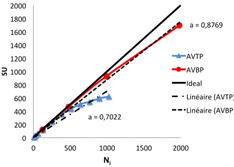
4.3.3 Practical example on an AVBP-AVTP coupled simulation . . . 73

4.4 Communication time between codes . . . 75

4.4.1 Toy description . . . 76

4.4.2 Case N1= N2. . . 78

4.4.3 Case N16= N2. . . 90

4.4.4 Towards realistic thermally coupled problems . . . 93

4.5 Conclusion . . . 96

II

Thermal state detailed analysis of a bluff-body stabilized laminar

pre-mixed flame

99

Contents

5.1 Numerical approach . . . 105

5.1.1 Studied configuration . . . 105

5.1.2 Computational method . . . 106

5.2 Flow characteristics description: baseline case . . . 108

5.3 Conclusion . . . 113

6 Variations of anchoring pattern as a function of the thermal state 115 6.1 Fluid-only approach: influence of the flame holder wall temperature . . . 116

6.1.1 Flame stabilization and flow field variations . . . 116

6.1.2 Impact on the bluff body wall fluxes . . . 120

6.2 Conjugate Heat Transfer: physical equilibrium states . . . 123

6.2.1 CHT results with a ceramic bluff-body . . . 124

6.2.2 Impact of solid conductivity on the equilibrium states . . . 127

6.3 Analysis of the convergence history of the coupled simulations . . . 134

6.3.1 Investigation of the numerical establishment of the different converged states obtained for Tinit= 1000 K . . . 135

6.3.2 Global convergence of all the CHT simulations . . . 140

6.4 Comparison with the results obtained with a chaining methodology derived from Errera & Chemin (2013) . . . 144

6.5 Conclusion . . . 147

III

Aerothermal prediction of an aeronautical combustion chamber

151

7.2 Numerical approach employed for the Combined Combustion Conduction and Ra-diation computation . . . 157

7.2.1 Solver setups . . . 157

7.2.2 Coupling strategy . . . 157

7.3 Combined Combustion Conduction and Radiation results . . . 158

7.4 Procedure validation by comparison with experiments . . . 160

chapter 0. CONTENTS

7.4.1 Comparison of the solid temperature map patterns . . . 160

7.4.2 Quantitative comparison on the outer envelop . . . 164

7.5 Conclusion . . . 166

General conclusion and perspectives 169 Bibliography 173 Appendices 191 A Large Eddy Simulation of reactive flows: equations and models 193 A.1 Compressible Navier-Stokes equations of multi-species reactive flows . . . 193

A.1.1 Momentum conservation . . . 193

A.1.2 Mass and species conservation . . . 194

A.1.3 Energy conservation . . . 196

A.2 Large Eddy Simulation . . . 197

A.2.1 Sub-grid closures and models . . . 197

Chapter 1

Scientific context

Contents

1.1 Working principle of a helicopter engine . . . 1

1.2 Heat transfer processes in a combustion chamber . . . 4

1.3 Multi-physic simulations . . . 6

1.4 Objectives and outline of the manuscript . . . 7

Because of progressive oil shortage, increasingly challenging environmental issues as well as a raising constraint of cost reduction, energy conversion through combustion has become a key current international concern. Since several years now, alternative solutions of renewable energy production more environmental friendly have born and developed in many industrial fields such as terrestrial transport or domestic energy supply. For air transport, such alternatives are today only at a very early development step. Indeed, the high power-to-weight ratio and autonomy required for aeronautical propulsion are today only achievable through hydrocarbon combustion. Addressing both environmental and cost constraints goes therefore through a better mastery of the combustion process. Tremendous efforts are thus deployed to better understand and control all the phenomena at play and produce cleaner and more efficient engines.

The work presented in this manuscript is the result of this specific context. It was funded by Turbomeca-SAFRAN to investigate and produce new methods to support the development of new generations of helicopter gas turbines.

1.1

Working principle of a helicopter engine

After some decades of very different concept trials, all gas turbines basic features as they are known today were clearly established by the beginning of the 1950s (Lefebvre, 2010). These devices are composed of an air intake, one or more compressor stages, a burner, one or more turbine stages and an exit nozzle (Fig. 1.1). Despite this similar global composition of all gas turbines, the specific

chapter 1. Scientific context

characteristics of every components vary with the applications (electrical power production, jet engine, turboshaft). For helicopter engines, restraining constraints of weight and compactness as well as an ability to operate on a very large range of conditions, lead more specifically to the common use of the following components (Fig.1.1):

. an air intake designed to ensure the proper conditions at the compressor inlet,

. few stages of compressors (usually centrifugal) operated by a shaft running through the engine and driven by the high pressure turbine,

. an annular reverse-flow combustion chamber allowing both engine compactness and a close coupling between the compressor and the turbine (avoiding hence shaft whirling problems), . several turbine stages converting gas kinetic energy into power, including a high pressure turbine and several stages of low pressure turbines driving respectively the compressors and the rotor, . an exit nozzle. Compressor Stages Combustion Chamber High-Pressure Turbine Co-Axial Shaft Low-Pressure Turbine stages Reducer Air Inlet

Figure 1.1: Cut view of Turbomeca’s Ardiden engine.

While flowing in these various components, the flow undergoes successive thermodynamic changes illustrated by the Brayton cycle (Fig. 1.2). In this ideal case, the air flow entering the engine undergoes an isentropic compression in the compressor stages (1-2), then the isobaric combustion

1.1. Working principle of a helicopter engine process adds heat into the system (2-3), burnt gases go through an isentropic expansion in turbine stages (3-4) and finally exhaust in an isobaric process to the atmosphere (4-1). In this ideal cycle, the net output power supplied by the engine for a given mass flow rate corresponds to the difference between the work required to drive the compressor and the work gained in the turbine stages and is proportional to the area limited by the 1-2-3-4 curve in Fig.1.2. Besides, the Brayton cycle efficiency ⌘ is defined as the ratio between the net output power and the input heat (due to combustion). In the absence of pressure and heat losses, this quantity reads:

⌘ = 1 − ✓ P2 P1 ◆γ−1 γ (1.1) where Pi is the pressure at the point i of the cycle and γ the gas polytropic exponent. At constant

Volume Pre ssu re Heat out Expansion Compression Heat in Baseline

Increased power and efficiency

1

2 3

4

Figure 1.2: Ideal Brayton cycle.

output power, increasing the cycle efficiency thus goes through an increase of the pressure ratio P2

P1 in the compressor stages. Such a feature however, leads to increased temperatures in the

com-bustion chamber and in the turbine stages. Over the years, gas turbine pressures have risen from 5 to 50 atm with resulting inlet and outlet temperatures respectively going from 450 to 900 K and from 1100 to 1850 K. At the same time expectations for life duration of flame tube liners have increased from a few hundred hours to several tens of thousands of hours, imposing drastic design constraints to these components (Lefebvre,2010).

The mechanical stresses experienced by the burner liner are small compared to those undergone for instance by rotating components. However, combustion chamber solid parts encounter very high levels of temperature and large thermal gradients that threaten material durability. In mod-ern gas turbines, hot gases in the combustion chamber can reach temperatures of the order of 2500 K. Such temperatures are far above the melting temperature of the materials forming the combustion chamber liner and injection system. Additionally, for the nickel-based or cobalt-based

chapter 1. Scientific context

alloys commonly used, a sharp decrease of the mechanical strength is observed for temperatures above 1100 K (Lefebvre, 2010). Therefore, the natural cooling of the liner through radiation and convection on the casing side is not sufficient to evacuate the heat transferred to the walls on the flame tube side of the liner and to decrease the temperature to an acceptable level. Specific cooling devices are required to cool down the metallic materials and prevent hot gases direct impingement onto the walls.

The required efficiency of such systems has raised over the years. Indeed, the increase of pressure ratios motivated by efficiency gains lead to larger burner inlet temperatures that reduce the casing air ability to cool down the walls by convection. In parallel, the pressure raise in the combustion chamber leads to larger heat transfers by radiation between the hot gas and the wall, further increasing the liner temperature. Finally, decreasing the levels of NOx emission has mainly been answered through leaner combustion, leading to more air being allocated to combustion. The amount of wall cooling air must hence be minimized to maximize the air available for emission control. All these constraints call for an optimization of wall cooling to find the optimal trade-off between performance of the engine and resistance of the components. However, this requires a detailed knowledge of the metal temperatures and thermal stresses experienced by the combustion chamber solid parts.

Today, complex thermocolor tests allow engine designers to access temperature fields on the in-ternal and exin-ternal walls of the flame tube. However, this experimental approach imposes some limitations such as the number of prototypes that can be tested and more importantly the few diagnostics made available. To limit such expensive experiments and integrate the knowledge of the thermal environment earlier in the design process, efforts are currently performed to provide high fidelity numerical tools able to predict the combustion chamber wall temperature. Such simulations would provide a path to get out from the trial and error process by allowing an easier determination of the mechanisms responsible for specific and undesired aerothermal response of the combustor. For the numerical resolution of such a thermal problem, one needs to consider the three heat transfer modes existing in nature, namely convection, radiation and conduction.

1.2

Heat transfer processes in a combustion chamber

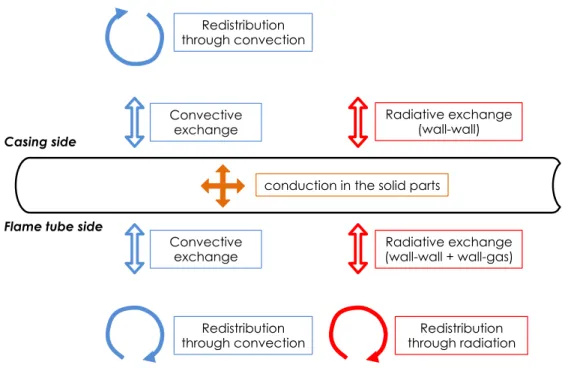
In a combustion chamber, energy exchange within the fluid and the solid as well as between the two domains is achieved simultaneously through the three existing modes of heat transfer. A schematic representation of these thermal exchanges is provided in Fig.1.3. Broadly, convection and radiation redistribute energy within the fluid and heat or cool the liner respectively on the flame tube and casing sides. Note that the relative magnitude of these two modes of heat transfer between the fluid and the solid depends on the burner configuration and operating conditions (Lefebvre, 2010). Finally, in reaction to the thermal stresses applied by the fluid, heat is

1.2. Heat transfer processes in a combustion chamber ported in the solid domain through conduction within the liner. To resolve the thermal problem in a combustion chamber one needs to consider all these heat transfer processes as well as the energy production through the chemical reactions. All these four processes are tightly coupled and each phenomena bounds the evolution of the others.

conduction in the solid parts Redistribution through convection Radiative exchange (wall-wall) Convective exchange Redistribution through convection Convective exchange Radiative exchange (wall-wall + wall-gas) Redistribution through radiation Casing side

Flame tube side

Figure 1.3: Thermal exchanges within the fluid and the solid domains as well as between the two domains.

Numerical tools allowing the numerical resolution of these processes independently in a burner exist since several years now. In particular, to compute the turbulent combustion phenomena (including both convection and energy production due to combustion), three main approaches are available which differ mainly by the respective amount of direct resolution and modeling that is to be provided. By decreasing amount of modeling and increasing associated computational cost, these are: Reynolds Averaged Navier-Stokes (RANS) simulation, Large Eddy Simulation (LES) and Direct Numerical Simulation (DNS) (Pope, 2000; Poinsot & Veynante, 2005). Depending on the flow properties, the geometry, the level of details required, as well as the nature of the target application, the various approaches may/may not be affordable and may/may not provide accurate solutions and sufficient information. While RANS flow simulation is the less expensive method and has thus been used for years, its accuracy is limited by the quality of its models. In the context of reactive flows that are strongly affected by turbulence and the inherent mixing, the use of RANS approaches in configurations as complex as current industrial burners showed some precision limitations and designers turn today more and more towards high fidelity techniques such

chapter 1. Scientific context

as LES. Indeed, the latter is less limited by associated models and can take great advantage of the increasing available computing power. LES is now widely accepted as the reference approach for burner flow simulations (Mahesh et al., 2001; Tucker & Lardeau, 2009) and will be used for the current study. In the same manner, various numerical methods exist to solve the radiative heat transfer and the solid conduction problems in combustion chambers.

However, most numerical studies reported in the literature are limited to the investigation of a single physical sub-system, neglecting the interactions with contiguous domains and with other physics within the same domain. At best these standalone simulations integrate some interactions with the environment through constant physical quantities determined with raw physical phenom-ena approximations or extracted from experiments as well as from other standalone simulations. None of these approaches, however, allow an effective resolution of the various interactions be-tween the different physical sub-systems. These independent simulations, though sufficient for the study of several phenomena may suffer from serious limitations. In some cases, improving the numerical resolution accuracy of a single sub-component seems to be of limited interest as long as the interactions between the sub-system and its environment is approximately defined. There-fore, a challenging path of improvement explored since several years now lies in the realization of multi-physics simulations in which the interactions between different physical sub-systems are actually solved.

1.3

Multi-physic simulations

Research on multi-physics thermal problems for combustion applications is relatively new and has greatly developed in the last decades. However, most existing studies include the coupling of com-bustion and either solid conduction or the radiative phenomena but not both. Such three physics simulations have however been reported byMercier et al.(2006) in a RANS context for the simu-lation of an industrial burner and three physics simusimu-lations including a LES solver were performed byAmaya (2010). In this last study, the solid domain was limited to the injection device, pre-cluding any investigation of the three physics effect on the combustion chamber liner temperature.

The resolution of such multi-physics problems jointly in the fluid and the solid domains can be done numerically through the use of two main approaches: monolithic and partitioned coupling. Monolithic techniques consist in producing a new solver handling the resolution of all the con-sidered phenomena within the same computational structure. In other words, this is a all-in-one solver. Such approaches though appealing especially when strong interconnections exist between the sub-system physics, may induce performance and scalability loss for specific sub-systems such as the LES resolution of the flow whose performance relies on specific data structures and solvers. On the contrary, the partitioned approach relies on the development of a coupled framework in which pre-existing codes are used to solve each physical sub-system. This allows the use of

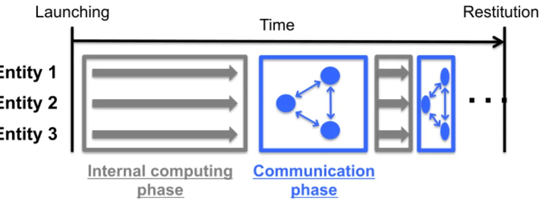
1.4. Objectives and outline of the manuscript ficient code structure and numerical methods specifically adapted to each set of equations. The solvers are then coupled through information exchange at the sub-system interfaces. In terms of performance, and to actually benefit from such a partitioned context, coupled applications require the use of a highly scalable code coupler to handle the coupled framework created around the various independent solvers. Besides, the computational cost mismatch between the sub-systems needs to be correctly handled to avoid any loss of performance. In such a context, the use of unsteady LES solvers, generally very scalable but highly computer ressource consuming increases performance constraints.

1.4

Objectives and outline of the manuscript

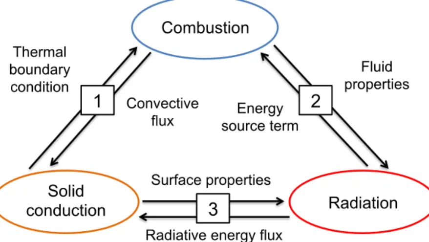
The work is motivated by the will to provide a high-fidelity solution of the thermal problem in a combustion chamber by considering all the means by which energy is exchanged and produced within the system. For this purpose, three codes solving the three heat transfer modes are coupled to investigate the interactions between the various physics in a combustion chamber: a high fidelity Large Eddy Simulation (LES) reacting flow solver, an unsteady solid conduction code and a Discrete Ordinate Method (DOM) radiation solver. Both scientific and engineering issues are investigated. More precisely, the various objectives targeted in this study are successively addressed through the following organization:

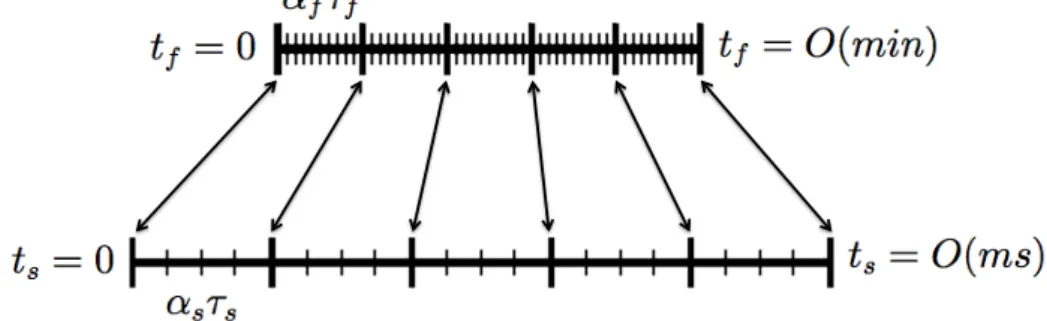
. PARTI: In this introductory part, the three physics at play when investigating the thermal state of a combustion chamber, namely combustion in the fluid domain, conduction within the chamber solid parts as well as radiative heat transfer in the fluid and at walls are suc-cessively discussed. The intrinsic different nature of these three processes and the resulting various resolution approaches (modeling approaches, specific assumptions and models) are detailed. Modeling of the interactions between the three physics is then addressed. In this context and acknowledging findings from the literature, several issues are discussed. First, in this manuscript, only mean quantities representative of the permanent regime are sought for. Starting from an initial condition, the simulation consists hence in computing all the sub-system interactions during a transient until the permanent regime is reached. However and since the various phenomena considered are characterized by very different time scales, such a computation of the full transient is not affordable in terms of computational cost and specific techniques are thus deployed. Second, the choice of the interface variables is critical both in terms of solution accuracy and computation stability and has to be done carefully. Coupling strategies chosen to handle both issues are thus discussed. Finally, a specific issue lies in the computational cost mismatch handling between the sub-systems. The impact of computing parameters on coupled simulations scalability is investigated in terms of coupling performance as well as computing resource distribution between the codes. The informatic and numerical implementation of coupled simulations having been addressed in this part, the two remaining parts of the manuscript focus on physical investigations of the interactions

chapter 1. Scientific context

in two different burner devices.

. PARTII: In numerical simulations of reactive flows, thermal boundary conditions are rarely well known and are thus treated mostly either as being adiabatic or at approximately fixed isothermal conditions. Such approximations on thermal boundary conditions can lead to sev-eral errors and inaccurate predictions of the combustion chamber flow field. In many cases, the wall thermal fields have a significant impact on the reactive flows, especially through the flame stabilization process. To validate the added value of a Conjugate Heat Transfer (CHT) approach in this context and evaluate the coupled aerothermal solution proposed, a simplified academic case is first studied. A detailed investigation of the thermal behavior of a laminar premixed flame stabilized thanks to a square cylinder in a channel flow (Kedia & Ghoniem, 2014a,b, 2015) is proposed. For this purpose, various standalone fluid DNS as well as coupled CHT simulations are performed. Such an academic configuration although more representative of some canonical laboratory burner than industrial aeronautical com-bustors allows deeper understanding and identification of the phenomena involved and their interactions without raising issues on potential modeling effects.

. PARTIII: To properly evaluate the thermal environment of combustors, combustion, con-duction and radiation should be taken into account as well as a realistic thermal modeling of the multiperforated walls. Besides, and in light of the literature results, the use of a LES flow solver is required to perform accurate burner coupled simulations. In this context, an objective of this work is to provide an evaluation of the solid steady state temperature field in a helicopter engine combustor while assessing the contribution of the different heat transfer mechanisms. For this purpose, various standalone and coupled simulations are per-formed. These include a reference adiabatic fluid-only simulation, and three multi-physics coupled simulations: Conjugate Heat Transfer (CHT), Radiation-Fluid Thermal Interaction (RFTI) and Combined Combustion, Conduction and Radiation (3CR) simulations. The various coupled simulations allow an evaluation of the interactions between all the physical sub-components. Note finally that for these exercise, the prediction capabilities of the meth-ods is assessed through comparisons between experimental results and coupled simulations.

Specific elements of the work performed during this PhD thesis were published in the following articles:

Berger, S., Richard, S., Staffelbach, G., Duchaine, F. & Gicquel, L.Y.M. 2015 Aerothermal prediction of an aeronautical combustion chamber based on the coupling of Large Eddy Simulation, solid conduction and radiation solvers. ASME Turbo Expo 2015: Turbine Tech-nical Conference and Exposition, Montr´eal, Quebec, Canada.

Berger, S., Richard, S., Staffelbach, G., Duchaine, F. & Gicquel, L.Y.M. 2016 On the sensitivity of a helicopter combustor wall temperature to convective and radiative thermal loads. Applied Thermal Engineering In press.

1.4. Objectives and outline of the manuscript Berger, S., Duchaine, F. & Gicquel, L.Y.M.2016 Influence des conditions aux limites ther-miques sur la stabilisation d’une flamme laminaire pr´em´elang´ee. Congr´es Fran¸cais de Thermique. Berger, S., Richard, S., Duchaine, F. & Gicquel, L.Y.M. 2016 Variations of anchoring pattern of a bluff-body stabilised laminar premixed flame as a function of the wall temperature. ASME Turbo Expo 2016: Turbine Technical Conference and Exposition, Seoul, South Korea.

Part I

Introduction

To answer the current objective of investigating the thermal state of a burner and perform highly performant multi-physics coupled simulations, several topics are to be addressed and are succes-sively discussed in this part. First, the physical specificities of combustion, solid conduction and radiation as well as the resulting numerical methods and models employed for their numerical resolution needs to be recalled. Having determined the approaches used for the independent reso-lution of the three phenomena, the resoreso-lution of the thermal problem required then the inclusion of the interactions between the sub-systems. In the partitioned coupling approach retained for the present computations, this is achieved via a regular exchange of specific physical quantities between the solvers. In such a context and to perform accurate and stable coupled simulations at an affordable computational cost, the treatment of the time and length scales disparities between the sub-systems as well as the choice of the interface variables is critical. Coupling strategies developed to handle these issues are thus discussed in this part. Finally, an additional dispar-ity between the sub-systems arise from the very different computational cost associated to the resolution of the various physical phenomena. Such a feature has to be correctly addressed by the coupling methodology to avoid computational resource waste and achieve highly performant coupled simulations.

All the issues highlighted here are discussed in this first part. The physics and the numerical methods employed to solve combustion, solid conduction and radiation are briefly recalled in Chapter 2. The coupling strategy between the sub-systems is then discussed in Chapter 3, ac-knowledging various studies from the literature. Finally, questions relative to coupled simulation performance are addressed in Chapter4.

Chapter 2

Physical problem and numerical resolution of the combustion,

solid conduction and radiation phenomena

Contents

2.1 Reactive flows . . . 16 2.1.1 Flow physics and numerical resolution . . . 16 2.1.2 Numerics in the AVBP solver . . . 24 2.1.3 Multi-species reactive flows . . . 25 2.2 Solid conduction . . . 25 2.2.1 The heat equation . . . 26 2.2.2 Numerics in the AVTP solver . . . 27 2.3 Radiative heat transfer . . . 28 2.3.1 The Radiative Transfer Equation (RTE) . . . 28 2.3.2 Resolution in PRISSMA . . . 33 2.4 Conclusion . . . 36

When investigating the thermal state of a burner, three physics are to be considered, namely combustion in the fluid, conduction within the chamber solid parts as well as radiative heat trans-fer in the fluid and at walls. As already mentioned in the introduction (Chapter1), the current multi-physics partitioned approach relies on the resolution of these three phenomena with differ-ent dedicated codes namely AVBP, AVTP and PRISSMA to solve respectively combustion, solid conduction and radiation. These three phenomena are intrinsically different. Their resolution relies on different approaches, assumptions and models, specific to each physics.

In this chapter, the physics of the three independent problems is described as well as the associated numerical resolution methods. All these physics and various existing resolution strategies in terms of numerics and modeling are the subject of very well written reference books and previous PhD thesis manuscripts. The description of the resolution method of each physics is restricted here to the approaches developed in the codes selected for the present study and emphasis is made

chapter 2. Combustion, solid conduction and radiation

on specific issues linked to the present multi-physics approach. Reactive flows are the focus of Section2.1 followed by the heat transfer through solid conduction and radiation respectively in Sections2.2and 2.3.

2.1

Reactive flows

The reactive flow within a burner is in itself a multi-physics problem and the combustion process results from complex two-way couplings between the fluid motion, species and heat diffusion as well as chemical reactions. As a result, the consideration of such a phenomenon requires the inclusion of both fluid mechanics and chemistry. The resolution of a fluid mechanics problem, even in a non-reactive context is already a complex task in itself and is first discussed in the present section. The consideration of a multi-species flow and the inclusion of chemical reactions is addressed in a second time. Note that when solving a reactive flow problem, the strong relation between the flow and the chemical reactions motivates the usual joint consideration of both phenomena within the same solver. Only a brief description of the physical phenomena and their numerical resolution is presented here. All these developments and further details can be recovered in text books such asPope (2000) (non-reactive flows) orWilliams(1985) andPoinsot & Veynante(2005) (reactive flows).

2.1.1

Flow physics and numerical resolution

Viscous flows can be phenomenologically separated in two categories: laminar and turbulent flows1. Such a property characterizes the flow regime and is determining for its resolution.

Flow regime: laminar versus turbulent

The drastic difference between laminar and turbulent flows was in particular highlighted by Reynolds in 1883 with a simple experiment (Reynolds, 1883) illustrated in Fig. 2.1. He injected a thin stream of dye into a water pipe flow and observed the effect of increasing the flow rate. At low flow rates, the dye stream trajectory was well-defined and parallel to the pipe axis. Its diameter very slightly increased when flowing downstream. As the flow rate was increased over a threshold value, the dye path spreads towards the pipe walls, following three dimensional ir-regular motions. Reynolds observed that the transition from one behavior to another occurred within a fixed range ([2000 − 3000]) of what is called today the Reynolds number and denoted Re (Reynolds, 1894). This non-dimensional number evaluates the ratio between inertia and viscous

1

Valuable observation of both flow regimes is proposed through numerous photographs of different simple

con-figurations inVan Dyke(1982).

2.1. Reactive flows forces and is nowadays widely used to characterize flow regimes:

Re = U L

⌫ (2.1)

where U and L are characteristic velocity and length scale of the flow and ⌫ the fluid kinematic viscosity. A low Reynolds number indicates a flow dominated by viscous forces and is thus

char-Figure 2.1: Reynolds’s experiment. From (Kundu et al., 2011).

acteristic of laminar flows while a high Reynolds number corresponds to a turbulent flow where inertial forces are predominant. The range of Re for which the flow switches from one regime to the other is usually referred to as the transitional regime and is very dependent on the configura-tion.

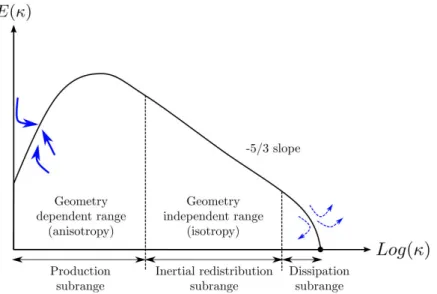
While laminar flows are characterized by regular paths with fluid particles moving in parallel layers, turbulent flows have an apparent random three dimensional behavior. They are composed of eddies of multiple length-scales (and time-scales) ranging from the integral length scale comparable to the flow scale to the Kolmogorov length-scale characteristic of the smallest eddies. Turbulent kinetic energy is produced in the largest structures and then transferred gradually to smaller and smaller scales through unsteady eddies stretching and break up. At the Kolmogorov scale, inertia and viscous forces balance, the kinetic energy contained in the smaller eddies eventually dissipates into heat. This fluctuation energy cascade principle was first formalized by Richardson in 1922 (Richardson, 1922) then by Kolmogorov (Kolmogorov et al., 1937) and is the key of the current understanding of turbulence. A graphical representation of this concept is provided in Fig. 2.2

chapter 2. Combustion, solid conduction and radiation

where a schematic turbulent flow energy spectrum is shown as a function of the wavenumber .

Figure 2.2: Turbulent energy spectrum as a function of the wave number . From (Fransen,2013) At a high Reynolds number, a separation of scales can be assumed (Pope,2000). While the large scale motions control the flow transport and mixing and are strongly geometry dependent, the small scales behavior is mostly controlled by the fluid viscosity and the energy received from the large scales. Therefore, the latter are known to have universal and only diffusive properties. Due to the effective transport and mixing ensured by large turbulent scales, turbulent flows are much more sought after in industrial applications than laminar flows. Besides, turbulence also enhances heat exchange rates at fluid-solid interfaces and are thus favored for numerous internal cooling applications.

Despite the strong phenomenological differences between laminar and turbulent flows, both regimes can be mathematically described with the same set of equations. These equations and their reso-lution are discussed in the next paragraph.

Flow resolution

The flow dynamics was first described mathematically by Euler in 1757 (Euler, 1757) for inviscid fluids. Sixty five years later, Navier introduced a viscosity coefficient in the equations (Navier,

1822). Finally, after contributions from various scientists through the years, Stokes published in 1845 the conservative equations for viscous fluids in their current form (Stokes, 1845) known as the Navier-Stokes equations.

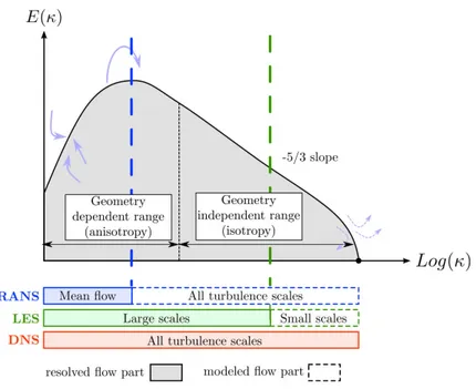
2.1. Reactive flows Due to its highly non-linear nature, this set of equations rarely gives right to analytic solutions. Instead, flow problems are spatially discretized on computational grids and solved numerically. For such purposes, an additional complexity arises in the context of turbulent flows: all the flow time and length scales are described in the balance equations leading thus to a huge amount of information to be resolved on the computational mesh. As a result, solving the full equations over the whole turbulence spectrum is not achievable (in terms of computing capabilities) in general. To overcome this issue and solve the flow field at an affordable CPU cost, various resolution approaches have been developed during multiple years of research. These differ mainly by the respective amount of direct resolution and modeling that is to be provided. In general, the complexity and the associated CPU cost increase with the level of details provided by each method. In addition, depending on the flow properties (Reynolds number), the geometry, the level of details required, as well as the nature of the target application, the various approaches may/may not provide accurate solutions and sufficient information. Three of the leading computational formalism for turbulent flows are discussed here: Direct Numerical Simulation (DNS), Large Eddy Simulation (LES) and Reynolds Averaged Navier-Stokes (RANS) simulation. For each method, the respective parts of the turbulence spectrum which are resolved or modeled are summarized in Fig.2.3.

Figure 2.3: Turbulent energy spectrum as a function of the wave number and various approaches modelisation domain. From (Fransen, 2013)

Direct Numerical Simulation

chapter 2. Combustion, solid conduction and radiation

over the entire spectrum or equivalently for the full range of spatial and time scales (Fig. 2.3). When considering non-reactive flows2_{, DNS are thus model free and often assimilated to}

numeri-cal experiments. This approach has provided very valuable insight into the understanding of the complex non-reactive and reactive turbulent flows and allowed for instance to produce efficient combustion models (Poinsot,1996;Chen et al.,2006;Chen,2011). However, such a full resolution of the turbulent flow requires a specifically defined grid with extremely small cell sizes (to resolve the smallest scales). In industry like applications, at least three orders of magnitude separate the flow system size from the mesh size needed to resolve the smallest eddies (Bockhorn et al., 2009), therefore precluding the use of DNS in such flows. This approach is for now limited to simplified geometries and laminar or low Reynolds number turbulent flows (because the computational cost increases as Re3 (Pope, 2000)). In other words, only academic applications can be pursued with this method. In this manuscript, a DNS approach is employed to compute an academic laminar bluff-body flame which is then used to go deeper in the understanding of thermal multi-physics simulations.

In most practical turbulent applications, it is not feasible to resolve all relevant scales explicitly and models are introduced to reduce the dynamic range of scales to solve and to account for influences of unresolved features on the resolved quantities. Two main classes of modeling are today present and described hereafter: RANS and LES.

Reynolds Averaged Navier-Stokes

This approach developed in the sixties aims at solving the mean flow values while modeling all the turbulent fluctuations. The RANS set of equations is obtained by time or ensemble averaging the Navier-Stokes balance equations. Therefore, variables are subdivided into an explicitly resolved part (mean quantity) and an unresolved modeled part covering the entire turbulence spectrum Fig.2.3. The production of both turbulent and turbulent combustion models (for reactive flows) is thus needed to properly account for the impact of the fluctuation fields on the mean. This mod-eling process has received extensive attention from the scientific community both in non-reactive (Pope, 2000) and reactive contexts (Poinsot & Veynante, 2005; Bockhorn et al., 2009).

RANS simulations provide a global knowledge of the flow mean repartition at a reduced CPU cost. Over the past decades, such numerical tools have been increasingly integrated into the design pro-cess of industrial devices such as aeronautical engines. Moreover, the reduced restitution times encountered with such techniques allowed their extensive use in optimization processes (Duchaine et al., 2009b), hence reducing drastically the number of experimental tests required during the development of industrial devices. Despite such clear advantages and because of the indubitable dependency of the large turbulent structures on the flow geometry, RANS simulations are some-what limited by the required adaptation of turbulence and turbulent combustion models to the

2

reactive flows require in addition the use of a chemical model

2.1. Reactive flows specificities of the flow considered. In addition, in reactive flows that are inherently affected by mixing, the use of RANS approaches in configurations as complex as current industrial burners showed some precision limitations and designers turn today more and more towards high fidelity techniques such as LES.

Large Eddy Simulation

Just like in RANS approaches, LES provides a solution to the Navier-Stokes equations at a re-duced CPU cost compared to DNS by resolving some features of the turbulent flow while modeling others. However, the resolved part is much consequent in LES: the large scales which contain most of the energy and are application dependent are resolved (Fig.2.3) and modeling is reduced to the smaller dissipative scales known to have a more universal behavior and costly to resolve. Since this approach relies on the universality of the small scale behavior, models are much less dependent on the considered application. As a main consequence, LES offers more predictivity capabilities than RANS.

The LES set of equations results from a spatial filtering of the Navier-Stokes equations: the large structures are resolved while all the scales of the turbulent flow below the filter length scale are fil-tered out. Due to the filtering of non-linear terms in the balance equations, sub-grid scale closures are needed which raises additional unknown terms which need to be modeled. In practice the scale separation between resolved and modeled features is often achieved directly via the computational mesh. Therefore, the more refined the mesh is the smaller are the resolved turbulent scales. As a result, for a given configuration, an increase of the computing capacity allows theoretically to include more and more resolution (with smaller and smaller cells) and less and less levels of mod-elisation. This specific point is a prerequisite for the development of SGS models which should hence tend towards zero as the grid resolution increases towards that required for DNS.

Originating from the meteorologic scientific field in the sixties (Lilly, 1966; Deardorff,1970), this approach developed significantly in the last decades with the increase of computing power. In-deed, the computational overhead induced by LES compared to RANS computations is substantial. First, performing accurate LES imposes more demanding grid refinement constraints, leading to meshes with larger number of points and cells. Second, the resolution of the Navier-Stokes equa-tions through such a high fidelity method requires the use of specifically designed highly precise numerical schemes providing both low numerical dissipation and low dispersion errors. This can be achieved with high order schemes that however induce additional computational costs. Note that the numerical resolution of the equations in the code AVBP is briefly discussed in the follow-ing. Finally, for statistically stationary flows, several flow through times are to be computed to obtain the flow mean fields (time averaged) further enlarging the overall cost of the simulation. As an example, the LES computation of a single sector of a helicopter annular combustion chamber requires around 50000 CPU hours, while a corresponding RANS computation would be dozen

chapter 2. Combustion, solid conduction and radiation times less CPU consuming.

Despite its increased cost, the valuability of LES for burner development has very recently led to the increased integration of such methods into the design phase. For the development of Tur-bomeca combustion chambers for instance, the number of LES computations in 2012 represented only 10% of the number of RANS computations performed. In 2015, the trend completely re-versed and RANS simulations represented only 5% of the total number of numerical simulations carried out at Turbomeca. Besides, the unsteady nature of LES provides possibilities to study transient phases such as ignition and extinction. Several attempts have been made to confront LES solutions of increasingly complex configuration against experimental results and provided very satisfying results (Gicquel et al., 2012). Still, this approach is relatively new and numerous developments from various research teams are still ongoing.

This approach is used in this manuscript to solve for the fluid flow in a multi-physics context and evaluate the thermal environment of an industrial burner for which DNS is clearly out of reach. However in such a complex and highly turbulent configuration, the resolution of the large energy containing turbulent scales in the viscous wall region is computationally unaffordable. Instead, the near-wall motions are modeled. In the present study, a classic wall-law approach is employed and described in the next paragraph.

Near-wall flow modeling

Wall treatment plays a crucial role in the prediction of wall-bounded flows. In LES of high Reynolds industrial applications, fully resolved turbulent boundary layers are not affordable due to the grid resolution required to accurately compute the shear stress and heat fluxes at walls. Wall laws based on boundary layer theory and inherited from RANS approaches (Schlichting,

1955; Cebeci & Cousteix, 2005) are therefore commonly used to account for the near-wall flow behavior and accordingly compute these quantities. Note that different approaches exist in the literature such as zonal approaches for which the near-wall flow is solved with a separate set of equations or hybrid RANS/LES methods (Piomelli, 2008). Various wall-laws exist with more or less complex formulations. The specific wall-law employed in this manuscript for the LES of an industrial burner is detailed below. Further details regarding the implementation in the solver AVBP can be found in (Schmitt,2005).

Wall flows are generally described with normalized wall variables. Introducing the wall shear stress:

⌧w= (µ@u/@y)w (2.2)

where µ is the fluid dynamic viscosity, u and y respectively stand for the tangential velocity and the direction normal to the wall and the subscripts w refers to wall quantities, one defines the

2.1. Reactive flows friction velocity:

uτ = p

⌧w/⇢ (2.3)

with ⇢ the fluid density. The normalized distance to the wall y+ as well as the normalized velocity u+ then read respectively:

y+= yuτ

⌫ (2.4)

u+ = u

uτ (2.5)

where ⌫ is the kinematic viscosity. If a wall modeled approach is to be retained, these normalized quantities are then linked through the so-called wall laws.

The turbulent boundary layer is characterized by its thickness δv, depending on the Reynolds number of the flow and is decomposed into an external layer (y/δv ≥ 0.2) controlled by turbulence, and an internal thin viscous layer (y/δv  0.2), itself made of 3 sub-layers:

. The first layer, for y+ 5, is the viscous sub-layer, where u+follows a linear function of y+. . The layer 40  y+ 300 according to (Cebeci & Cousteix,2005) corresponds to the inertial

layer, characterized by the well-known log law given by:

u+= 1/ ln(y+) + C1 (2.6)

where  = 0.41 is the Karman constant determined experimentally (von K´arm´an,1930) and C1= 5.4 for internal flows.

. Between these two layers is an intermediate zone commonly called buffer zone, where tran-sition between the linear and the log law occurs. In this zone neither the linear nor the log law is accurate. In AVBP, a threshold value y+ _{= 11 is fixed under which the linear law is} used while for superior values the log law is used.

The thermal aspect of near-wall modelisation can be treated in a similar way. In this case, a friction temperature, similar to the friction velocity is introduced:

Tτ = Qw ⇢ Cp uτ

(2.7) where Qw is the wall heat flux and Cp the fluid heat capacity. Then, a non-dimensional tempera-ture reads:

T+= Tw− T

Tτ (2.8)

chapter 2. Combustion, solid conduction and radiation

The normalized temperature follows the same two zone principle than the normalized velocity, with a linear region and a log region:

. in the viscous sub-layer (y+  5),

T+ = P r y+ (2.9)

. for 40  y+ 300, the Kader law is imposed (Kader, 1981): T+= P rt

 ln(y +

) + C2 (2.10)

with P r and P rt respectively the molecular and turbulent Prandtl numbers. P r_κt is fixed here to 2.12 and C2 depends on the molecular Prandtl number: C2= (3.85 P r1/3− 1.3)2+ 2.12 ln(P r). In addition to the specific treatment of the near-wall flows, and as previously mentioned, a key issue for the realization of high-fidelity simulations lies in the numerical formalism employed for the resolution of the balance equations. The numerical choices made in the AVBP solver are briefly described in the next paragraph.

2.1.2

Numerics in the AVBP solver

The LES/DNS code AVBP solves the compressible reacting Navier-Stokes equations for momen-tum, mass and energy conservation on unstructured hybrid grids. The solver is based on a finite volume cell-vertex formulation and relies on an explicit time integration approach. A second order Galerkin scheme is used in all the present simulations for the resolution of the diffusion terms (Don´ea et al., 2000). The convective terms are resolved thanks to two different classes of numerical schemes:

. A Lax-Wendroff (LW) (Lax & Wendroff, 1960) scheme, second-order accurate in time and space which provides a fairly good accuracy at a low computational cost. This scheme tends however to provide less accurate dispersion and dissipation properties for medium-to-high wave numbers.

. Two different Taylor-Galerkin schemes: TTGC (Colin & Rudgyard, 2000) and TTG4A (Quartapelle & Selmin, 1993) third-order accurate in space and third-order (TTGC) or fourth-order (TTG4A) accurate in time. Both schemes ensure better dissipation and dis-persion properties than the LW scheme. Note however that this improved accuracy has a significant cost: Simulations performed with TTGC or TTG4A are around 2.5 more CPU consuming than LW computations.

Further details concerning the numerical methods implemented in AVBP can be found in ( Lamar-que,2007).

2.1. Reactive flows The time explicit integration implies a control of the time-step by the limiting acoustic Courant-Friedrichs-Lewy (CFL) condition. For a given value of the CFL, the time step is given by

∆tf =

CF L ∆x

u + cs (2.11)

where u is the local convective velocity and csthe local speed of sound. In a perfect gas, the speed of sound depends on the fluid properties and reads,

cs= r

γRT

M (2.12)

with γ the ratio of specific heat, R the ideal gas constant, T the temperature and M the gas molar mass.

2.1.3

Multi-species reactive flows

The description of multi-species reactive flows requires in addition to the resolution of the non-reactive Navier-Stokes equations, the calculation of chemical source terms as well as the resolution of a transport equation for each mixture species. The full Navier-Stokes equations governing reac-tive flows are briefly recalled in AppendixA. In AVBP, reduced kinetic schemes are developed to account for chemical reactions. Classic Arrhenius laws are used to compute reaction rates which are then used to determine the energy and species source terms.

When dealing with reactive turbulent flows, additional complexities come from the strong rela-tions that lie between chemical reacrela-tions and turbulent mixing (Peters & Rogg, 1993). On one hand, turbulence is modified by the combustion process through changes of flow properties (den-sity and visco(den-sity) with local temperature as well as acceleration of the flow through the flame front due to heat release. On the other hand, turbulence stretches and wrinkles the flame front, thus affecting the consumption rate and the flame local propagation speed. These interactions are highly non-linear and can cause antagonist effects. As an example, flame stretching and wrinkling due to turbulence can lead to an incredibly higher consumption rate whereas a too high stretch and wrinkling can lead to local quenching and eventually blow-off of the entire flame. These interactions are the topic of a huge amount of studies (Poinsot & Veynante, 2005) and accurate numerical resolution of turbulence/combustion interactions is still an open topic. Indeed, while in a DNS framework, the flame as well as its interactions with turbulent mixing is explicitly resolved, the use of RANS or LES approaches introduces the need for turbulent combustion models. Some usual models are reviewed inPoinsot & Veynante(2005) orPitsch(2006) and the specific method of flame thickening employed for the present study is briefly described in AppendixA.

chapter 2. Combustion, solid conduction and radiation

combustion chambers (Poinsot & Veynante, 2005). Indeed, an efficient and fast mixing of fresh reactants enhance the combustion process while improved mixing between burnt and fresh gases helps the burnt gases cooling process and hence prevents critical hot spot impingement onto the turbine blades. Note also that turbulence increases the heat transfer between the flow and the walls which is of particular interest for the present study.

2.2

Solid conduction

Energy transfers by conduction happen without transfer of mass. This process spontaneously appears when a temperature gradient occurs within a material system. Heat conduction in solids is a diffusion-type problem and can be described mathematically through the so-called heat equation. Most of the notions detailed here can be found in reference books such as B´edat & Giovannini

(2012) or Taine & Petit(1995).

2.2.1

The heat equation

Heat diffusion in solid materials is governed by the heat equation. Fourier established this equa-tion in 1822 (Fourier, 1822) by decomposing the problem into three different components: heat storage within a small solid element, heat transport in space and exchanges between the interior and the exterior through boundary conditions (Narasimhan, 1999). A fascinating review of this work, the scientific context in which Fourier established this equation as well as the derived ben-efits in numerous diffusion-type problems applied to various scientific fields (electricity, chemical diffusion ...) can be found inNarasimhan(1999).

In the absence of internal heat source, the unsteady heat equation reads: @⇢CT

@t = [r · (λrT )] (2.13)

with

. T the temperature, . ⇢ the density,

. C the specific heat capacity (material ability to store energy),

. λ the thermal conductivity (material ability to transport heat) considered homogeneous (isotropic conduction).

These material properties are linked through the thermal diffusivity which characterizes the ma-terial ability to respond to external perturbations (here imposed by the fluid through convection

2.2. Solid conduction and radiation),

a = λ

⇢ C. (2.14)

In AVTP, the temperature dependency of the specific heat capacity C and the thermal conduc-tivity λ is approximated with polynomial laws whose parameters depend on the material. When physical properties are constant the heat equation becomes linear and simplifies to:

@T

@t = ar

2

T (2.15)

Finally, for a stationary problem, the heat equation reduces to the Laplace equation:

r2T = 0 (2.16)

This equation is independent from the material thermal conductivity. In this specific case, solu-tion uniqueness is ensured as long as appropriate boundary condisolu-tions are provided. Considering an unsteady problem, an additional initial condition is required to solve the system.

Boundary conditions can be defined through three different mathematical formulations. Note that hereafter subscript w refers to the problem unknown at the boundary condition while subscript ref corresponds to a quantity that is prescribed at the boundaries.

Dirichlet boundary condition

Temperature is imposed at the wall surface:

Tw= Tref (2.17)

Neumann boundary condition

The heat flux is imposed at the wall surface: qw= −λ ✓ @T @n ◆ w = qref (2.18)

Note that a stationary problem including only Neumann boundary conditions is not well posed (B´edat & Giovannini, 2012): i.e. infinite set of solutions.

Robin boundary condition

The heat flux is imposed with a relaxation term:

qw= qref + kref(Tref − Tw) (2.19)