O
pen
A
rchive
T
OULOUSE
A
rchive
O
uverte (
OATAO
)
OATAO is an open access repository that collects the work of Toulouse researchers and
makes it freely available over the web where possible.
This is an author-deposited version published in :
http://oatao.univ-toulouse.fr/
Eprints ID : 19578
To link to this article : DOI:
10.1109/TPS.2017.2777835
URL
http://dx.doi.org/
10.1109/TPS.2017.2777835
To cite this version : Goussard, Valentin and Duprat, Fançois and
Gerbaud, Vincent and Nardello-Rataj, Véronique and Aubry, Jean-Marie
and Ploix, Jean-Luc and Dreyfus, Gérard: Predicting the Surface Tension
of Liquids: Comparison of Four Modeling Approaches and Application
to Cosmetic Oils (2017), Journal of Chemical Information and Modeling,
vol. 57, n°12, pp.2986-2995
Any correspondance concerning this service should be sent to the repository
administrator:
[email protected]
Predicting the Surface Tension of Liquids: Comparison of Four
Modeling Approaches and Application to Cosmetic Oils
Valentin Goussard,
†François Duprat,
*
,‡Vincent Gerbaud,
§Jean-Luc Ploix,
‡Gérard Dreyfus,
‡Véronique Nardello-Rataj,
†and Jean-Marie Aubry
*
,††Univ. Lille, CNRS, Centrale Lille, ENSCL, Univ. Artois, UMR 8181 - UCCS - Unité de Catalyse et Chimie du Solide, F-59000 Lille,
France
‡Laboratoire de Chimie Organique, CNRS, ESPCI Paris, PSL Research University, 10 rue Vauquelin, 75005 Paris, France §Laboratoire de Génie Chimique, Université de Toulouse, CNRS, INP, UPS, 31432 Toulouse, France
ABSTRACT: The efficiency of four modeling approaches, namely, group contributions, corresponding-states principle, σ-moment-based neural networks, and graph machines, are compared for the estimation of the surface tension (ST) of 269 pure liquid compounds at 25 °C from their molecular structure. This study focuses on liquids containing only carbon, oxygen, hydrogen, or silicon atoms since our purpose is to predict the surface tension of cosmetic oils. Neural network estimations are performed from σ-moment descriptors as defined in the COSMO-RS model, while methods based on group contributions, corresponding-states principle, and graph machines use 2D molecular information (SMILES codes). The graph machine approach provides the best results, estimating the surface tensions of 23 cosmetic oils, such as hemisqualane, isopropyl myristate, or decamethylcy-clopentasiloxane (D5), with accuracy better than 1 mN·m−1. A demonstration of the graph machine model using the recent Docker technology is available for download in the Supporting Information.
1. INTRODUCTION
Surface tension (ST) is the force existing at a liquid/gas interface, which tends to minimize the surface area; it is caused by asymmetries in the intermolecular forces between molecules located at the interface. It plays an important role in a number of processes where a liquid/gas interface is present; for instance, it drives the shape of small liquid drops and bubbles or the wetting of a solid surface by a liquid.1In cosmetics, the spreadability of oils on the human skin reflects both the sensory qualities and the efficacy of the product;2,3 Parente et al. reported that the spreadability of oils and thefilm forming properties could be partly correlated to the surface tension of the cosmetic oil:2the lower the surface tension, the more spreadable the oil.
Surface tensions can be measured by numerous methods (e.g., Wilhelmy plate, Du Noüy ring, maximum bubble pressure, drop-weight, or hanging-drop) accounting for the large amount of experimental data available in the literature.4 However, for a given compound, significantly different surface tension values can be found, depending on the method used and/or the purity of the liquid. Furthermore, when virtual liquids are generated in silico,5the experimental determination of surface tension is not possible. In this case, it is crucial to predict reliably the surface tension values of candidate compounds in order to select the most promising ones, which should be synthesized first. Unfortunately, predicting this property is not straightforward because of the complexity of the phenomenon, i.e., the necessity to break bonds in order to bring a molecule from the bulk phase
to the surface.6Various prediction methods for surface tension values were described previously by several authors.1,6−11
In this paper, four modeling approaches, namely, group contributions, corresponding-states principle,σ-moment-based neural networks, and graph machines, are applied to the prediction of the surface tension of liquid compounds. These methods are described below.
Molecular dynamic simulations werefirst used in 1976, when Rao et al. highlighted the possibility of computing the surface tension of a liquid film from statistical thermodynamic relations.12In 2016, Ghoufi et al. calculated the surface tension by modeling the liquid/gas interface.13Density functional theory has also been used successfully for the surface tension prediction of 18 pure nonpolar fluids.14 Nevertheless, models based on molecular dynamics are computer demanding and not suitable for structures with more than a few tens of atoms such as some we are interested in.
Introduced by Brock and Bird in 1955,15the corresponding-states principle allows surface tension estimations from the critical constants Pc, Vc, and Tc. Curl and Pitzer improved this model, which is restricted to short and weakly polar molecules by introducing an acentric shape parameter.16Escobedo et al. used this model for the surface tension prediction of 94 compounds,17
and Li et al. presented a new method based on a combination of corresponding-states and group contribution models.18
Group contribution-based (GC) methods are popular approaches to predict a wide range of physicochemical properties.19,20 In such methods, the molecular structure of any organic compound is viewed as an assembly of functional groups with specific property attributes. The properties of the studied molecule are computed as a function of the contributions of the different groups, with respect to their occurrence (first-order contribution), with respect to adjacent groups (second order), and with respect to other molecular attributes (third order). Regarding the prediction of surface tension, a model was introduced by Egemen et al. in 2000 to predict the surface tension of 44 organic compounds,21and an extended model was proposed by Conte et al.7
Models based on quantum chemistry are also effective to predict a wide range of physicochemical properties of organic compounds. In particular, the COSMO-RS method (Conductor-like Screening MOdel for Real Solvents), introduced by Klamt in 1995, is based on unimolecular quantum chemical calculations combined with exact statistical thermodynamics.22−24It provides the necessary information for predicting chemical potentials in liquids, from which one can compute many other thermody-namic equilibrium properties such as activity coefficients, solubility, partition coefficients, vapor pressure, and free energy of solvation,25 without requiring any experimental input. For instance, the interfacial tension between two liquids, i.e., the free energy per unit surface area that is required for maintaining an interface between two condensed phases, can be calculated using COSMO-RS.26 However, the prediction of surface tensions remains a challenge, yet unsolved by COSMO-RS (Klamt personal communication). Interestingly, Kondor et al. proposed to predict surface tensions at different temperatures by a regression method, using the so-called Klamt set of COSMO-RS σ-moments. This set of five descriptors is well known to encode as much chemical information as the complete set of 15 COSMO-RSσ-moments. The five σ-moments calculated from the σ-profiles of the molecules under study22,25,27 and the temperature were selected as inputs of a nonlinear Quantitative Structure−Property Relationship (QSPR) model,6 based on neural networks.
QSPR models are regression or classification models that predict a property of a molecule from selected descriptors thereof; they were used successfully for the prediction of surface tensions of a wide range of organic compounds.1Kondor et al. used a data set of 1275 surface tension values, collected at different temperatures for 188 molecules, for building and validating the model. When the model was applied to a test set of 225 data points, the squared correlation coefficient R2between the estimated surface tensions and the experimental values was equal to 0.96. Stanton et al. described a 10-descriptor model for the prediction of surface tensions of 146 compounds.8 Kauffmann et al. developed a model based on eight descriptors for a data set of 159 molecules.9 Freitas et al. decreased the number of descriptors of the model to six to successfully predict the surface tensions of 299 compounds.10Delgado et al. designed a model with six descriptors corresponding to the different intermolecular interactions in the bulk phase and calculated from the molecular structures1 for the prediction of the surface tensions of 320 compounds.
Goulon et al. developed graph machines as an alternative QSAR/QSPR method.28 Graph machines are regression or classification models that estimate properties of molecules
directly from the topological information supplied by their SMILES (Simplified Molecular Input Line Entry Specification) codes. Therefore, they do not require any descriptor. In these models, molecules are described as graphs derived from their 2D-structure, and the parametrized functions that compute the estimation of the property or activity of interest reflect the compound molecular structures. As usual in regression or classification models, the parameters of the graph machines are computed during training from examples present in a database of experimental values of the property or activity of interest. The main benefit of the method is the absence of descriptors, with the SMILES codes being the only required information.
In the present work, surface tension estimations are performed by four different methods, falling into two families: (i) group contribution models and corresponding-states principle models (Section 2.1) and (ii) neural network regression and graph machine regression (Section 2.2). Neural network regression is performed from COSMO-RSσ-moments, whose computation is described inSection 2.3. For thefirst family, methods are taken from the literature. For the two methods of the second family, predictive models are designed and trained from a database of surface tensions, at 25°C, of 269 molecules belonging to several chemical families and containing only carbon, hydrogen, oxygen, and silicon atoms, namely, alkanes, ethers, esters, ketones, carbonates, acids, alcohols, silanes, and siloxanes, with straight, branched, or cyclic chains. For all four methods, the predictive ability of the resulting models are assessed by the estimation of the surface tensions of 23 cosmetic oils that are not present in the training data set.
2. EXPERIMENTAL AND THEORETICAL METHODS
2.1. Group Contribution and Corresponding-States Based Models. Surface tension estimations using methods based both on group contribution (GC) or on the correspond-ing-states principle (CSP) were carried out using the InBioSynSolv (IBSS) property library developed by Heintz et al.29IBSS software is intended to design new molecules satisfying targeted properties and to predict many physicochemical properties by means of methods encoded in a property model library.7,29 Among the methods available in IBSS for the prediction of surface tensions, the Conte et al. GC method7 was developed by splitting 402 molecules into chemical groups and estimating the parameters of the following relation:
∑
∑
∑
= + + ST NC M D O E i i i j j j k k k (1)where ST is the surface tension, Ci, Dj, and Ek are the first-, second-, and third-order contributions estimated by successive linear regressions, and Ni, Mj, and Okare the occurrences of the molecular groups. The reported standard deviation of the estimation error (i.e., of the difference between the estimated and measured values of the surface tension) is 1.47 mN·m−1, and the mean absolute estimation error is 1.05 mN·m−1over the 402 data points of the database used for estimating the parameters Ci, Dj,
and Ek, in a range between 15 and 52 mN·m−1.7,30Once the contribution values are estimated, the GC method is intended to predict the property value of any molecular structure. Difficulties can appear when using such methods, e.g., a nonunique decomposition of some structures or compounds with fragments for which no group contributions have been defined yet. This is the case for siloxane derivatives, which are at the core of the present study.
Other estimation methods have been developed, based on the principle of corresponding states.31 This principle states that some dimensionless properties will follow the same relation over dimensionless variables of state and other dimensionless quantities for all compounds, typically, the reduced temperature (Tr= T/Tc) and reduced pressure (Pr= P/Pc), where Tcand Pc
are the critical temperature and pressure. The related CSP models are the so-called two-parameter corresponding-states principle relation. For surface tension, an additional parameter, Pitzer’s dimensionless acentric factor ω, was introduced to better match the CSP relation and the experimental data, leading to the following relation:16,32 ω ω ω = + + − − ⎡ ⎣⎢ ⎤⎦⎥ ST P T 1.86 1.18 T 19.05 3.75 0.91 0.291 0.08 (1 ) c2/3 1/3c r 2/3 11/9 (2)
Zuo and Stenby used an 86-component database containing almost exclusively hydrocarbons (linear and branched alkanes and alkenes, aromatics) to develop the model for the surface tension based on a CSP approach. It includes two reference fluids, methane and n-octane:33
= ⎛ + ⎝ ⎜⎜ ⎞⎠⎟⎟ ST ST P T ln 1 r c2/3 1/3c (3) ω ω ω ω = + − − − STr STr(1) (STr STr ) (1) (2) (1) (2) (1) (4) where = − STr(1) 40.520(1 Tr)1.287 (5) and = − ‐ ST T methane n octane 52.095(1 ) 1: ; 2: r(2) r 1.21548 (6)
In relations2and3, with the critical pressure and temperature expressed in bar and Kelvin, respectively, ST is obtained in mN· m−1. The authors claimed a five percent accuracy for nonpolar fluids and reported larger deviations for more polar substances. 2.2. Neural Network and Graph Machine Modeling. 2.2.1. Database Construction. The data set required for the training of neural networks and graph machines was carefully built with the following requirements in mind: (i) to obtain a representative sample of the surface tension variation with the chain length for compounds belonging to homologous families, (ii) to select molecules that contain the constitutional atoms usually found in the cosmetic oils, i.e., carbon, hydrogen, oxygen, and silicon, (iii) to select, for each molecule, at least two consistent measured values for the surface tension provided by different literature references, and (iv) to include only molecules that are in the liquid state at 25°C under atmospheric pressure. A data set of 269 molecules (hereinafter termed“complete set”) with a measured surface tension ranging from 12 to 48 mN·m−1 was built from data extracted from reliable sources34−38 and retrieved from technical datasheets.39,40 When measured data were not available at 25°C, but for several other temperatures nearby, a simple linear equation was used to interpolate the surface tension at 25°C.
2.2.2. Model Selection. Model selection is a crucial step in the design of machine-learning based models. Its purpose is tofind, given the available data, the appropriate model complexity that
provides the best generalization, i.e., that provides the most accurate estimations on data that are not present in the training set. The available data set of 269 molecules was partitioned into a training/validation set of 244 molecules and a test set of 25 molecules for performance assessment. The molecules of the test set were chosen so that (i) the distributions of molecules among the chemical families considered were very similar in the complete and test sets and that (ii) the distribution of the surface tension values was as uniform as possible on the range of measured values. The distribution of the molecules among chemical families is displayed inFigure 1.
Model selection was performed by computing the virtual leave-one-out score (defined inSection 3.2) of each model, at the end of the training process performed with the training/ validation set. Further details are provided inSections 2.2.3and
2.2.4.
After model selection, the performance of the selected neural network model and the performance of the selected graph machine model were assessed on the 25-molecule test set. As a final step, the surface tensions of 23 cosmetic oils were measured as described inSection 2.4and predicted by the neural network and the graph machine models as described inSection 3.3.
2.2.3. Neural Networks. A neural network is a nonlinear parametrized function.41 In the framework of nonlinear regression for estimating a quantity of interest from a training set of NTelements, the neural network parameters are estimated from available data during a training phase, which consists of minimizing the sum of squared training errors J(θ) with respect to the parameters
∑
θ = − θ = J( ) (y g( )) i N i i 1 2 T (7)where yiis the measured value of the quantity of interest for the
ith element of the training set, and gi(θ) is the value of the quantity of interest estimated by the neural network. In the present case, the quantity of interest is the surface tension of liquids, hence yiis the measured value of the surface tension of
molecule i of the database, gi(θ) is the estimated value of the surface tension of molecule i, and NT= 244 as explained in the
previous section. In the present study, the minimization of J(θ) was performed by the Levenberg−Marquardt algorithm.
For nonlinear regression by neural networks, the usual form of gi(θ) is a linear combination of nonlinear functions called Figure 1.Family distribution (as percentages) for the molecules of the complete (left) and test (right) data sets.
“hidden neurons”. Each hidden neuron is a continuous, nonlinear function (typically a tanh function) of a linear combination of the variables. Such a neural network is called a multilayer Perceptron (MLP). It is particularly suitable for nonlinear regression because it is a universal approximator: any continuous nonlinear function can be approximated with arbitrary accuracy by an MLP having afinite number of hidden neurons. An MLP with zero hidden neurons is a linear model, hence is trained by traditional least-squaresfitting.
As usual in nonlinear regression, the generalization ability of an MLP model depends on its complexity, which depends basically on the number of hidden neurons. A neural network with too many neurons approximates the training data very accurately but is unable to generalize, i.e., to predict accurately data that are not present in the training set; a neural network with too small a number of neurons is unable to learn the training data, hence to generalize (this phenomenon is known as the “bias-variance dilemma”). Therefore, the design of an MLP requires a model selection phase.39 In the present study, MLP selection was performed by virtual leave-one-out, as described inSection 3.2.
2.2.4. Graph Machines. As mentioned previously, a graph machine is intended to perform classification or regression on graphs; in QSAR/QSPR applications, the graphs under consideration are the 2D structures of the molecules. In the present case, a graph machine provides an estimate of the surface tension; the latter quantity being continuous, the task considered here is a regression task.
The design of a graph-machine based model includes the following steps:
• Construction of the 2D-graph of the molecule from its SMILES representation: Each node of the graph is a non-H atom, and each edge is a chemical bond of the graph. Each node has at least two labels: its nature and its degree (the number of chemical bonds that bind it to its adjacent non-H atoms). For molecules that contain cycles, hence are represented by a cyclic graph, edges are deleted in order to form an acyclic graph in which every path of the graph has its end at a specific node called “output node”. • Construction of the computational structure: For each acyclic graph, a function is generated by implementing, at each node of the graph, a parametrized nonlinear function, called node f unction (typically an MLP). All node functions are identical and have the same parameters within each graph and for all graphs; therefore, the number of parameters of the resulting model is equal to the number of parameters of the chosen node function. As a result of this construction, the value computed by the output node of each model, which is intended to be an estimate of the property of interest, depends solely on the 2D structure of the molecule and on the values of the parameters of the node function.
• Estimation of the parameters of the node function by training from the database: This is done by minimizing the sum of squared errors J(θ) defined inSection 2.2.3. Details of the above steps are provided in a previous paper42 and references therein. The bias-variance dilemma applies to graph machines as well as to any machine learning method, so an appropriate model selection procedure must be performed. The selection method for graph-machine based models is described in
Section 3.2.
2.3. COSMO-RS Computing Procedure. COSMO-RS uses a combination of quantum chemistry and statistical
thermody-namics in order to compute the chemical potentialμ of a solute in a liquid phase, which can then be converted into physicochemical properties.22As mentioned in theIntroduction, no model for the estimation of surface tension is available from COSMO-RS yet. An alternative approach consists in using descriptors provided by COSMOtherm: the so-called COSMO-RSσ-moments.
Because of polar covalent bonds, molecules bear a charge densityσ on the so-called σ-surface, which is a slightly inflated van der Waals surface of the compound. The full 3D information about the charge density repartition on the σ-surface can be reduced to a curve pX(σ), the σ-profile of the molecule X, which is
a smoothed histogram expressing how much of theσ-surface lies in the polarity interval [σ − dσ/2, σ + dσ/2].25Figure 2gives an
example of the σ-profiles of three cosmetic oils: propylheptyl caprylate, dioctyl ether, and n-tetradecane. None of these compounds has Lewis acidity (hydrogen-bond (HB) donor region), but Lewis basicity (HB acceptor region) is present. The σ-profiles show the difference in the Lewis basicity, propylheptyl caprylate having the strongest one since the curve exhibits the most significant peak above 0.01 e.Å−2.
Klamt suggested an expression of the partition coefficient K of a solute X between two phases as a development on the σ-moments (eq 8).22Usually, a development to m = 6 is sufficient to estimate satisfactorily the partition coefficient K.
∑
= + +
= RTlnK c Macc accX c Mdon donX c M
i m
i iX
0 (8)
Theσ-moments MiXare calculated from theσ-profiles pX(σ) of
the studied compound X, according toeqs 9−11:
∫
σ σ σ σ = − σ + +∞ MaccX pX( )( HB)d HB (9)∫
σ σ σ σ = − − σ −∞ − MdonX HBpX( )( HB)d (10)∫
σ σ σ = −∞ −∞ MiX pX( ) id (11)Among the 15σ-moments, the first ones have a simple physical meaning. The zero-orderσ-moment M0Xis the whole surface area
of the molecule, expressed in Å2. Thefirst-order one M1Xis the
polarization charge of this surface, expressed in e. For uncharged molecules, this moment is equal to zero. The second-order
σ-Figure 2. Plots of σ-surfaces and σ-profiles of three cosmetic oils: propylheptyl caprylate (blue), dioctyl ether (red), and tetradecane (green) using the COSMO-RS model.
moment M2X, expressed in e2·Å−2, is the polarity of the studied
molecule.27The third-order M3Xrepresents the asymmetry of the
σ-profile pX(σ). The other σ-moments M 4 X, M 5 X, and M 6 Xhave no
known physical meaning. Finally, MaccX and MdonX , expressed in e,
are the “hydrogen-bonding” σ-moments. They represent the ability of the molecule to interact with hydrogen-bond acceptors and donors, respectively. They have a nonzero value when the σ-profile of a molecule outstrips the range [−σHB, +σHB], whereσHB
is the hydrogen-bond cutoff equal to 0.01 e·Å−2.
The 14not 15 since M1X is always equal to zero for the
uncharged molecules of our studycalculated σ-moments values for the complete and test sets of molecules are given in Tables S3 and S4 of theSupporting Information.
2.4. Surface Tension Measurements for Cosmetic Oils. To assess the accuracy of the estimations of the developed model, a test data set of 23 cosmetic oils that are not present in the complete set was built. The surface tensions of these cosmetic oils were determined experimentally, using two different methods: measurements were both performed (i) with the Krüss K100 tensiometer which measures the force occurring when a probe (ring, plate or rod) is completely wetted with a liquid and (ii) by the pendant drop method associated with the Krüss DSA10 tensiometer. It has thus been verified on a few molecules that values obtained for surface tensions are consistent from one method to the other. The values measured with the K100 tensiometer at 23.5°C are presented inTable 3. The rod is immersed in each liquid studied, with an immersion rate of 10 mm·min−1and an immersion depth of 2 mm. The force acting on the rod is recorded and allows the calculation of the surface tension of the liquid. Before each series of measurements, calibration with pure water is carried out. Additionally, surface tensions of four liquids belonging to the training/validation set, whose values (reported in the literature) can be found in Table S1 of the Supporting Information, were measured for the following results (all values with a standard deviation of 0.2 mN· m−1): n-undecane ST = 23.1 mN·m−1, n-pentadecane ST = 26.9 mN·m−1, triacetine ST = 35.1 mN·m−1, and decamethylcyclo-pentasiloxane ST = 18.0 mN·m−1. These values are consistent with those of the literature. During a liquid measurement, the surface tension values were sampled every 3 s until the standard deviation was below 0.1 mN·m−1. Three measurements were taken in a row for each sample. The means and standard deviations of the measurements performed on the 23 compounds are reported in Table S2 of the Supporting Information. No temperature correction was made to the previous measured values since the observed deviations between 0.1 and 0.7 mN·m−1were larger than the temperature corrections, expected to be below 0.2 mN·m−1.
3. RESULTS AND DISCUSSION
3.1. Dependence of Surface Tension on Chemical Function and Chain Length. The variation of the surface tensions of several chemical families (alkanes, ethers, esters, ketones, carbonates, acids, alcohols, silanes, and siloxanes) with the number of carbon atoms is plotted inFigure 3, gathering experimental values from at least two independent sources. For silicon-containing compounds, the variation of the surface tension is plotted against the sum of the number of carbon and silicon atoms. For instance, decamethylcyclopentasiloxane (C10H30O5Si5) is plotted at abscissa 15 on the X-axis ofFigure 3. For all chemical families, the surface tension increases with the number of carbon or (carbon+silicon) atoms. Surface tension is closely related to the intermolecular forces: the stronger these
forces, the more tightly bound the molecules, hence the higher the surface tension. Because long chains are more likely to form more intermolecular bonds than small ones do, the surface tension increases with chain length. Silicones exhibit drastically low surface tension. This is due to their inorganic polar backbone on which apolar organic groups are grafted, able to rotate freely around the Si−O bonds. These apolar groups shield the Si−O backbone, preventing the dipolar interactions thereby decreasing the surface tension. Apart from silicones, alkanes and ethers have the lowest surface tensions because only London interactions take place between CH2/CH3groups. Compounds containing
polar ester groups have higher surface tensions because of the Keesom and Debye interactions. Finally, alcohols have higher surface tension values because these molecules carry a free hydroxyl group that is involved in strong intermolecular hydrogen bonds. As explained in theIntroduction, a low surface tension results in high spreadability. That is why silicones are used in cosmetic formulations.Figure 3gives an indication on how chemical functions affect the surface tension of linear molecules, showing that alkanes and ethers are the carbon compounds whose surface tensions are closest to those of silicones. It also focuses on the effect of chain length on the surface tension for series of linear molecules (except cyclic silicones), highlighting the increase in intermolecular forces with the chain length, responsible for an increase in surface tension. Obviously, this property does not depend only on those two factors, but also on topological modifications such as cyclization or branching of compounds. Thus, results presented in the following sections of this study also deal with branched and cyclic compounds.
3.2. Modeling Surface Tensions of the Liquids of the Complete Set. 3.2.1. Surface Tension Estimation from σ-Moments by Neural Networks (Multilayer Perceptrons). In the present section, we discuss the design and test of a multilayer Perceptron for the estimation of the surface tension of the molecules of the complete data set described inSection 2.2.1, comprising 269 compounds that carry diverse functional groups (ethers, ketones, acids, carbonates, esters, silanes, siloxanes, alkanes, and alcohols) and that possess straight or branched chains, cycles, etc. The compounds contain only carbon, hydrogen, oxygen, and silicon atoms because those are the
Figure 3.Variation of the surface tensions (ST) for various families of linear molecules: alkanes (blue circles), ethers (empty purple circles), acetates (red triangles), alcohols (empty orange triangles), and carboxylic acids (yellow crosses) with the number of carbon atoms and with the sum of carbon and silicon atoms for Si-containing compounds (green squares for linear silicones and empty brown squares for cyclic silicones).
only atoms present in the backbone of cosmetic oils. The database was partitioned into a training/validation set of 244 compounds and a test set of 25 compounds as described in
Section 2.2.3. In the spirit of Kondor et al.,6the estimation was performed by a multilayer Perceptron fromfive COSMO-RS σ-moments: M0, M2, M3, Macc, and Mdon. [Neural network computations were performed with a homemade software package based on the NeuroOne kernel, a former product of Netral S.A.] Feature selection by the random probe method41 confirmed the fact that for our data M0, M2, and M3are the most relevant for ST estimation.
Model selection was performed by training models of increasing complexity (number of hidden neurons).39For each model complexity, 100 models were trained with different random initial parameter values. The Root Mean Square Training Error (RMSTE) and the Virtual Leave-One-Out (VLOO) score were computed:
θ = RMSTE J N ( )m T (12)
where J(θ) is the sum of square errors (eq 7),θmis the vector of
parameters of the model after completion of training, and NT=
244 is the number of molecules in the training/validation set:
∑
θ = − = − VLOO score N y g 1 [ ( )] T i N i i 1 mi 2 T (13)where yiis the surface tension value measured for molecule i, and gi(θm−i) is the surface tension value for molecule i that would have
been estimated by the model if molecule i had been left out the training set (i.e., if the model had been trained on all molecules of the training/validation set except molecule i). The virtual leave-one-out score provides an unbiased estimation of the general-ization ability of the model.43The 10 models (out of 100) having the smallest VLOO scores were stored.
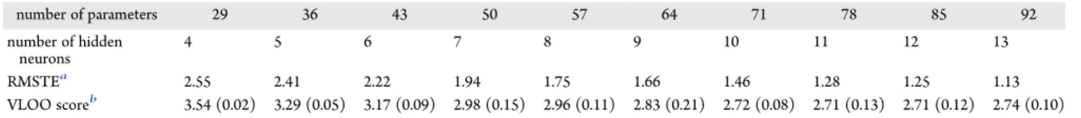
The third row ofTable 1shows the values of the RMSTE on the 244 molecules of the training/validation set for the best trained models (models with minimum RMSTE) of increasing complexity. As expected, RMSTE decreases monotonously with increasing complexity; by contrast, the mean value of the VLOO scores of the 10 stored models (fourth row) first decreases, reaches a minimum for the model with 78 parameters (multilayer Perceptron with 11 hidden neurons), and subsequently increases. This illustrates the bias-variance dilemma explained inSection 2.2.3. The VLOO score difference between the 71- and 78-parameter models is very small, and the recommended practice in such a situation is to select the most parsimonious (least complex) model. Therefore, the multilayer Perceptron with 10 hidden neurons was selected for testing. The results of the models with less than four hidden neurons are not displayed, as they have much higher values.
For the selected modelwith 10 hidden neuronsthe VLOO ST estimates for molecules of the training/validation set and the ST estimates for the molecules of the test set are plotted against their measured values inFigure 4. The RMSE
computed for the training/validation and test sets are equal to 1.91 and 3.60 mN·m−1, respectively, and the determination coefficients R2, displayed for both sets, are equal to 0.89 and 0.76,
respectively. The surface tension is correctly estimated around the center of the range but is clearly inadequate for the outer examples, which impairs the R2 value for the test set where outliers, being at the ends of the range, have large leverages.
As mentioned in theIntroduction, Kondor et al. were thefirst to use the COSMO-RSσ-moments for nonlinear regression by neural networks. To build their model, Kondor et al. used a database of 1500 surface tensions recorded for 188 molecules at different temperatures.6 The initial set was partitioned into a training/validation set of 1275 examples and a test set of 225 examples. The results, obtained with a neural network whose variables were the COSMO-RSσ-moments mentioned above, were fair for both sets. However, the method used for partitioning the set remains unclear since there are more examples in the test set than the number of initial molecules. Therefore, some compounds are inevitably in both sets at least once, though at different temperatures. This is clearly identified Table 1. Surface Tension Estimation fromσ-Moments by Neural Networks (Multilayer Perceptrons). Estimation of the Quality of Training and of the Predicting Ability for Increasing Neural Network Complexity
number of parameters 29 36 43 50 57 64 71 78 85 92 number of hidden neurons 4 5 6 7 8 9 10 11 12 13 RMSTEa 2.55 2.41 2.22 1.94 1.75 1.66 1.46 1.28 1.25 1.13 VLOO scoreb 3.54 (0.02) 3.29 (0.05) 3.17 (0.09) 2.98 (0.15) 2.96 (0.11) 2.83 (0.21) 2.72 (0.08) 2.71 (0.13) 2.71 (0.12) 2.74 (0.10) aRMSTE value (mN·m−1) of the model (out of 100) having the smallest RMSTE for the 244 molecules of the training/validation set.bMean and standard deviation (in parentheses) of the VLOO scores (mN·m−1) averaged over the 10 models (out of 100) having the smallest VLOO scores for
the 244 molecules of the training/validation set.
Figure 4. Surface tension estimation from σ-moments by neural networks. VLOO surface tension (ST) estimates computed by neural network (multilayer Perceptron with 10 hidden neurons) for the 244 molecules of the training/validation set (gray hollow circle) and surface tension estimates for the 25 molecules of the test set (blackfilled circle) vs measured values of the surface tension. The VLOO estimates for the molecules of the training/validation set and the estimates for the molecules of the test set are computed with the 10 models (out of 100) that have the smallest VLOO scores. The dashed gray line is the regression line for the training/validation set, while the dashed black line is the regression line for the test set.
for CO2, with three data points belonging to the training set and
one to the test set. A solid assessment of the prediction ability of Kondor’s model would request a test with fresh examples not pertaining to any of the previous sets and possessing known surface tension values at various temperatures. To the best of our knowledge, this is yet to be done.
3.2.2. Surface Tension Estimation from SMILES by Graph Machines. In the present section, we discuss the design and test of graph machines (described inSection 2.2.4) for the estimation of the surface tension of the molecules of the complete data set described in Section 2.2.1, comprising 269 compounds, and partitioned into a training/validation set of 244 compounds and a test set of 25 compounds.
The model design methodology for graph machines is the same as described inSection 3.2.1 for multilayer Perceptrons: graph machines of increasing complexity (number of hidden neurons of the node function) were trained. For each model complexity, 100 models were trained with different random initial parameter values. RMSTE (eq 12) and the VLOO scores (eq 13) were computed, and the 10 models having the smallest VLOO scores were stored.
The third row ofTable 2shows the RMSTE values of the best-trained models (models with smallest RMSTE) with different complexities for the 244 molecules of the training/validation set. As expected, the RMSTE decreases with increasing complexity, while the mean value of the VLOO scores of the 10 stored models (fourth row) goes through a minimum (model with 95 parameters, i.e., node function with seven hidden neurons) and subsequently increases. Therefore, graph machines with seven hidden neurons were selected for further testing.
As an illustration, the VLOO ST estimates for molecules of the training/validation set and the ST estimates for the molecules of the test set are plotted against their measured values inFigure 5. The RMSE computed for the training/validation and test sets are both equal to 0.77 mN·m−1, and the determination coefficients R2, displayed for both sets, are above 0.98. This demonstrates that the VLOO score on the training/validation set provides an accurate assessment of the generalization ability of the model. It also shows that the accuracy of the graph machine estimations is much better than the accuracy of MLP estimations from the σ-moments. Indeed, the estimation error of graph machines is on the order of the experimental uncertainty on the available data.
Tables gathering the results with both group contribution and corresponding-states based methods, and respective RMSE, are given in theSupporting Information.
3.3. Comparison of the Four Approaches on the 23 Cosmetic Oils Test Set. For further testing, the cosmetic oils set (23 molecules) was investigated. Most molecules display polar functions with oxygen. As such we may expect large deviation in the prediction with the Zuo and Stenby corresponding-states method that was developed over a database containing only nonpolar molecules. To take advantage of the
maximum information on all the available data, the complete set of 269 molecules was used as a training/validation set. For graph machines, 250 models with node functions having seven hidden neurons were trained from that set. The 25 models that had the smallest VLOO scores were applied to the cosmetic oils set, and the mean of their estimates of the surface tension was taken as the final estimate. This resulted in a RMS estimation error of 0.9 mN· m−1. For the MLP estimation from σ-moments, 250 models having 10 hidden neurons were trained from the same set. The 25 models that had the smallest VLOO scores were also applied to the cosmetic oils set, and the mean of their estimates of the surface tension was taken as thefinal estimate. The results are compared with those obtained with the other two methods, group contribution, and corresponding-states method. Devia-tions from experimentally measured values of surface tension are gathered inTable 3. Because of the absence of contribution for siloxane groups in Conte’s group contribution method, the surface tension for the dodecamethylcyclohexasiloxane (D6) cannot be estimated.
A large deviation is observed between the experimental data and the values predicted by the GC method. We notice that the molecules considered inTable 3have a larger molecular weight than compounds included in the database used for the predictions. Conte’s original paper did not give a list of data set molecules but provided several examples.7Not a single one concerned such large molecules. This hints at the fact that the Table 2. Surface Tension Estimation from SMILES by Graph Machines. Estimation of the Quality of Training and of the Predicting Ability for Increasing Graph Machine Complexity
number of parameters 31 44 59 76 95 116 139 164 number of hidden neurons 3 4 5 6 7 8 9 10 RMSTEa 1.99 1.33 0.94 0.75 0.49 0.40 0.31 0.18 VLOO scoreb 2.77 (0.08) 2.40 (0.15) 2.31 (0.27) 2.05 (0.21) 1.71 (0.29) 1.85 (0.26) 1.90 (0.26) 2.46 (0.77) aRMSTE value (mN·m−1) of the model (out of 100) having the smallest RMSTE for the 244 molecules of the training/validation set.bMean and standard deviation (in parentheses) of the VLOO scores (mN·m−1) averaged over the 10 models (out of 100) having the smallest VLOO scores for
the 244 molecules of the training/validation set.
Figure 5.Surface tension estimation from SMILES by graph machines. VLOO surface tension (ST) estimates computed by graph machines (node function with seven hidden neurons) for the 244 molecules of the training/validation set (gray hollow circle) and surface tension estimates for the 25 molecules of the test set (blackfilled circle) vs measured values of the surface tension. The VLOO estimates for the molecules of the training/validation set and the estimates for the molecules of the test set are computed with the 10 models (out of 100) that have the smallest VLOO scores. The dashed gray line is the regression line for the training/validation set, while the dashed black line is the regression line for the test set.
database set used to develop the GC model does not sample the space of molecules to which the test set we are interested in belongs.
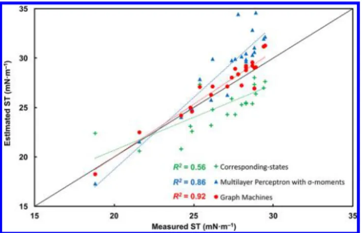
Thus, in the following, surface tensions estimated with the corresponding-states methods described by Zuo and Stenby are compared to results obtained with the neural networks and graph machines. Figure 6 presents the comparison between the experimentally measured surface tensions of the 23 cosmetic oils of the test set and the predicted surface tensions with
corresponding-states based method, neural networks using the COSMO-RSσ-moments as descriptors, and graph machines.
The method of corresponding states advocated by Zuo and Stenby performs poorly as was expected. For all but for two compounds, the surface tensions are grossly underestimated. The estimations by neural networks fromσ-moments are not very satisfactory, which suggests that the σ-moments do not contain sufficiently relevant information for our task. In particular, graph machines provide the most accurate estimation as they take into account the structure of the molecule, thereby Table 3. Difference between Measured and Predicted Surface Tension (ST) for 23 Cosmetic Oils
aMean measured surface tension values (ST) are reported in mN·m−1at 23.5°C.bDifference between measured and predicted ST using group contribution method implemented in the IBSS software.cDifference between measured and predicted ST using corresponding state-based method included in IBSS software.29 dDifference between measured and predicted ST using neural network model based on the five σ-moments.6 eDifference between measured and predicted ST using graph machines.26fThe root-mean-square error is computed witheq 13for the 23 molecules of the test set; the estimations for the surface tension are averaged over the 25 models (out of 250) that have the smallest VLOO scores for the multilayer Perceptron and the graph machines (71 and 95 parameters, respectively).gn/a: not applicable.
exempting the model designer from the computation and selection of features.
4. CONCLUSIONS
Predicting surface tensions of liquids fromfirst-principles is not straightforward due to the complexity of the interactions taking place at gas/liquid interfaces. It remains still inaccessible even by advanced methods such as COSMO-RS able to calculate accurately interfacial tensions between two liquid phases.26 In the present study, the estimation of surface tensions of cosmetic oils was performed by the group contribution method, by the corresponding-states method, by nonlinear regression (multi-layer Perceptron) from COSMO-RS σ-moments, and by regression on graphs (graph machines). To the best of our knowledge, this is thefirst study that compares the accuracy of various methods for estimating the surface tensions of the same molecules and where the models are tested on two sets of molecules; it is also thefirst report of the use of graph machines for surface tension estimation. The database of surface tensions was created with special emphasis on the diversity of the molecules and on the reliability of the experimental results. It was shown that the group contribution method failed to provide accurate estimations (root-mean-square estimation error = 6.7 mN·m−1); the corresponding-states method and nonlinear regression from σ-moments yielded estimations with similar accuracies (root-mean-square estimation errors = 2.4 and 2.7 mN·m−1respectively); graph machines, which make estimations solely from the molecular structure, provided the most accurate estimations (0.9 mN·m−1). Pending the development of methods, based onfirst-principles, for surface tension estimation only from molecular structures, graph machines are shown to be able to provide, from molecular structures, estimations whose errors are on the order of the experimental uncertainty on the available data. An interactive demonstration of the graph machine computations, based on the Docker free software technology (existing for many computer platforms) is available for download (see theSupporting Information). In the present study, all measurements were taken at the same temperature. As surface tension varies with temperature, we intend to use the ability of graph machines to take into account exogenous variables (e.g., temperature) for prediction.
■
ASSOCIATED CONTENT*
S Supporting InformationThe Supporting Information is available free of charge on the
ACS Publications websiteat DOI:10.1021/acs.jcim.7b00512. Names, SMILES notations, molecular formulas, CAS RN, σ-moment descriptors, and measured surface tensions values in mN·m−1at 25 °C of the 244 molecules of the training/validation set, the 25 molecules of the test set, and the 23 molecules of the cosmetic oil set; group-contribution Conte method estimated, corresponding-states Pitzer’s method estimated, corresponding-states Zuo-Stenby method estimated, neural network estimated, neural network VLOO estimated, graph machine estimated and graph machine VLOO estimated values of the surface tension in mN·m−1for the 269 molecules of the complete set; group-contribution estimated, neural net-work estimated, and graph machine estimated values of the surface tension in mN·m−1for the 23 molecules of the cosmetic oil set; Docker Client installation, graph machine demonstration with Docker containers and graph machine results with Docker. (PDF)
■
AUTHOR INFORMATION Corresponding Authors*Phone: 33-1-40794465. Fax: 33-1-40794466. E-mail: arthur. [email protected](F. Duprat).
*Phone: 33-3-20336364. E-mail:[email protected]
(J.-M. Aubry).
ORCID
François Duprat:0000-0002-2889-1701
Véronique Nardello-Rataj:0000-0001-8065-997X
Notes
The authors declare no competingfinancial interest.
■
ACKNOWLEDGMENTSOne of the authors (V. Goussard) thanks the company Oleon for financial support by means of doctoral fellowship.
■
REFERENCES(1) Delgado, E. J.; Diaz, G. A. A Molecular Structure Based Model for Predicting Surface Tension of Organic Compounds. SAR QSAR Environ. Res. 2006, 17, 483−496.
(2) Parente, M. E.; Gambaro, A.; Solana, G. Study of Sensory Properties of Emollients Used in Cosmetics and Their Correlation with Physicochemical Properties. Int. J. Cosmet. Sci. 2005, 56, 175−182.
(3) Parente, M. E.; Gambaro, A.; Ares, G. Sensory Characterization of Emollients. J. Sens. Stud. 2008, 23, 149−161.
(4) Gharagheizi, F.; Eslamimanesh, A.; Tirandazi, B.; Mohammadi, A. H.; Richon, D. Handling a Very Large Data Set for Determination of Surface Tension of Chemical Compounds Using Quantitative Structure−Property Relationship Strategy. Chem. Eng. Sci. 2011, 66, 4991−5023.
(5) Gharagheizi, F.; Eslamimanesh, A.; Mohammadi, A. H.; Richon, D. Use of Artificial Neural Network-Group Contribution Method to Determine Surface Tension of Pure Compounds. J. Chem. Eng. Data 2011, 56, 2587−2601.
(6) Kondor, A.; Járvás, G.; Kontos, J.; Dallos, A. Temperature Dependent Surface Tension Estimation Using COSMO-RS Sigma Moments. Chem. Eng. Res. Des. 2014, 92, 2867−2872.
(7) Conte, E.; Martinho, A.; Matos, H. A.; Gani, R. Combined Group-Contribution and Atom Connectivity Index-Based Methods for Estimation of Surface Tension and Viscosity. Ind. Eng. Chem. Res. 2008, 47, 7940−7954.
Figure 6.Predicted surface tension values computed by graph machine (red circles), neural networks based onfive σ-moments (blue triangles), and corresponding-states (green crosses) vs experimentally measured surface tension values for the test set of 23 cosmetic oils.
(8) Stanton, D. T.; Jurs, P. C. Computer-Assisted Study of the Relationship between Molecular Structure and Surface Tension of Organic Compounds. J. Chem. Inf. Model. 1992, 32, 109−115.
(9) Kauffman, G. W.; Jurs, P. C. Prediction of Surface Tension, Viscosity, and Thermal Conductivity for Common Organic Solvents Using Quantitative Structure- Property Relationships. J. Chem. Inf. Comput. Sci. 2001, 41, 408−418.
(10) Freitas, A. A.; Quina, F. H.; Carroll, F. A. A Linear Free Energy Analysis of the Surface Tension of Organic Liquids. Langmuir 2000, 16, 6689−6692.
(11) Albahri, T. A.; Alashwak, D. A. Modeling of Pure Compounds Surface Tension Using QSPR. Fluid Phase Equilib. 2013, 355, 87−91.
(12) Rao, M.; Levesque, D. Surface Structure of a Liquid Film. J. Chem. Phys. 1976, 65, 3233−3236.
(13) Ghoufi, A.; Malfreyt, P.; Tildesley, D. J. Computer Modelling of the Surface Tension of the Gas−liquid and Liquid−liquid Interface. Chem. Soc. Rev. 2016, 45, 1387−1409.
(14) Fu, D.; Lu, J.-F.; Liu, J.-C.; Li, Y.-G. Prediction of Surface Tension for Pure Non-Polar Fluids Based on Density Functional Theory. Chem. Eng. Sci. 2001, 56, 6989−6996.
(15) Brock, J. R.; Bird, R. B. Surface Tension and the Principle of Corresponding States. AIChE J. 1955, 1, 174−177.
(16) Curl, R. F.; Pitzer, K. Volumetric and Thermodynamic Properties of Fluids-enthalpy, Free Energy, and Entropy. Ind. Eng. Chem. 1958, 50, 265−274.
(17) Escobedo, J.; Mansoori, G. A. Surface Tension Prediction for Pure Fluids. AIChE J. 1996, 42, 1425−1433.
(18) Li, P.; Ma, P.-S.; Dai, J.-G.; Cao, W. Estimations of Surface Tensions at Different Temperatures by a Corresponding-States Group-Contribution Method. Fluid Phase Equilib. 1996, 118, 13−26.
(19) Marrero, J.; Gani, R. Group-Contribution Based Estimation of Pure Component Properties. Fluid Phase Equilib. 2001, 183−184, 183− 208.
(20) Constantinou, L.; Gani, R. New Group Contribution Method for Estimating Properties of Pure Compounds. AIChE J. 1994, 40, 1697− 1710.
(21) Egemen, E.; Nirmalakhandan, N.; Trevizo, C. Predicting Surface Tension of Liquid Organic Solvents. Environ. Sci. Technol. 2000, 34, 2596−2600.
(22) Klamt, A. COSMO-RS: From Quantum Chemistry to Fluid Phase Thermodynamics and Drug Design,first ed.; Elsevier: Amsterdam, The Netherlands, 2005.
(23) Klamt, A. Conductor-like Screening Model for Real Solvents: A New Approach to the Quantitative Calculation of Solvation Phenomena. J. Phys. Chem. 1995, 99, 2224−2235.
(24) Klamt, A.; Jonas, V.; Bürger, T.; Lohrenz, J. C. W. Refinement and Parametrization of COSMO-RS. J. Phys. Chem. A 1998, 102, 5074− 5085.
(25) Klamt, A.; Eckert, F.; Hornig, M. COSMO-RS: A Novel View to Physiological Solvation and Partition Questions. J. Comput.-Aided Mol. Des. 2001, 15, 355−365.
(26) Andersson, M. P.; Bennetzen, M. V.; Klamt, A.; Stipp, S. L. S. First-Principles Prediction of Liquid/Liquid Interfacial Tension. J. Chem. Theory Comput. 2014, 10, 3401−3408.
(27) Lukowicz, T.; Benazzouz, A.; Nardello-Rataj, V.; Aubry, J.-M. Rationalization and Prediction of the Equivalent Alkane Carbon Number (EACN) of Polar Hydrocarbon Oils with COSMO-RS σ-Moments. Langmuir 2015, 31, 11220−11226.
(28) Goulon, A.; Picot, T.; Duprat, A.; Dreyfus, G. Predicting Activities without Computing Descriptors: Graph Machines for QSAR. SAR QSAR Environ. Res. 2007, 18, 141−153.
(29) Heintz, J.; Belaud, J.-P.; Pandya, N.; Teles Dos Santos, M.; Gerbaud, V. Computer Aided Product Design Tool for Sustainable Product Development. Comput. Chem. Eng. 2014, 71, 362−376.
(30) Hukkerikar, A. S.; Sarup, B.; Ten Kate, A.; Abildskov, J.; Sin, G.; Gani, R. Group-Contribution+(GC+) Based Estimation of Properties of
Pure Components: Improved Property Estimation and Uncertainty Analysis. Fluid Phase Equilib. 2012, 321, 25−43.
(31) Poling, B. E.; Prausnitz, J. M.; O’Connell, J. P. The Properties of Gases and Liquids,fifth ed.; McGraw-Hill, 2001.
(32) Pitzer, K. S. Thermodynamics; McGraw-Hill, New York, 1995. (33) Zuo, Y.-X.; Stenby, E. H. Corresponding-States and Parachor Models for the Calculation of Interfacial Tensions. Can. J. Chem. Eng. 1997, 75, 1130−1137.
(34) Jasper, J. J. The Surface Tension of Pure Liquid Compounds. J. Phys. Chem. Ref. Data 1972, 1, 841−1010.
(35) Le Neindre, B. Tensions superficielles des composés organiques. Techniques de l’ingénieur; 1993; Vol. K477, pp 1−40.
(36) Yaws, C. L. Chemical Properties Handbook: Physical, Thermody-namic, Environmental, Transport, Safety, and Health Related Properties for Organic and Inorganic Chemicals; McGraw-Hill, New York, 1999.
(37) Wohlfarth, C.; Wohlfarth, B.; Landolt, H.; Börnstein, R.; Martienssen, W.; Madelung, O. Numerical Data and Functional Relationships in Science and Technology; New Series; Group 4, Vol. 16; Physical Chemistry Surface Tension of Pure Liquids and Binary Liquid Mixtures; Springer, Berlin, 1997.
(38) Haynes, W. M. CRC Handbook of Chemistry and Physics, 92 ed.; CRC Press, 2011.
(39) JEFFSOL Alkylene Carbonates, Comparative Solvents Data. Huntsman Corporation: The Woodlands, Texas, 1999.
(40) Dow Oxygenated Solvents; Form No. 327-00001 1014 MM; The Dow Chemical Company, October 2014.
(41) Dreyfus, G.; Neural Networks: Methodology and Applications; Springer, Berlin, New York, 2005.
(42) Dioury, F.; Duprat, A.; Dreyfus, G.; Ferroud, C.; Cossy, J. QSPR Prediction of the Stability Constants of Gadolinium(III) Complexes for Magnetic Resonance Imaging. J. Chem. Inf. Model. 2014, 54, 2718−2731. (43) Monari, G.; Dreyfus, G. Local Overfitting Control via Leverages. Neural Comput. 2002, 14, 1481−1506.