Trace Selection for Improved WLAN Monitoring

(1)

HAL Id: hal-00840829

https://hal.archives-ouvertes.fr/hal-00840829v2

Submitted on 2 Aug 2013

HAL is a multi-disciplinary open access

archive for the deposit and dissemination of

sci-entific research documents, whether they are

pub-lished or not. The documents may come from

teaching and research institutions in France or

abroad, or from public or private research centers.

L’archive ouverte pluridisciplinaire HAL, est

destinée au dépôt et à la diffusion de documents

scientifiques de niveau recherche, publiés ou non,

émanant des établissements d’enseignement et de

recherche français ou étrangers, des laboratoires

publics ou privés.

Trace Selection for Improved WLAN Monitoring

Matteo Sammarco, Miguel Elias Mitre Campista, Marcelo Dias de Amorim

To cite this version:

Matteo Sammarco, Miguel Elias Mitre Campista, Marcelo Dias de Amorim. Trace Selection for

Improved WLAN Monitoring. HotPlanet 2013 - 5th ACM HotPlanet Workshop, Aug 2013, Hong

Kong, Hong Kong SAR China. pp.9-14, �10.1145/2491159.2491165�. �hal-00840829v2�

(2)

Trace Selection for Improved WLAN Monitoring

Matteo Sammarco

UPMC Sorbonne Universités Paris, France

matteo.sammarco@lip6.fr

Miguel Elias M. Campista

Universidade Federal do Rio de Janeiro

Rio de Janeiro, Brazil

miguel@gta.ufrj.br

Marcelo Dias de Amorim

UPMC Sorbonne Universités Paris, France

marcelo.amorim@lip6.fr

ABSTRACT

Existing measurement techniques for IEEE 802.11-based net-works assume that the higher the density of monitors in the target area, the higher the quality of the measure. This assumption is, however, too strict if we consider the cost involved in monitor installation and the necessary time to collect and merge all traces. In this paper, we investigate the balance between number of traces and completeness of collected data. We propose a method based on similarity to rank collected traces according to their contribution to the monitoring system. With this method, we are able to select only a subset of traces and still keep the quality of the mea-sure, while improving system scalability. In addition, based on the same rank, we identify monitors that can be relo-cated to enlarge the monitored area and increase the overall efficiency of the system. Finally, our experimental results show that the proposed solution leads to a better tradeoff in terms of unique captured frames over the number of merge operations.

Categories and Subject Descriptors

C.2.3 [Computer-communication Networks]: Network Operations—network monitoring, network management

General Terms

Management, Design, Measurement, Experimentation

Keywords

Wireless networks; IEEE 802.11; measurement; monitoring; scalability

1. INTRODUCTION

Wireless monitoring systems typically employ multiple pas-sive sensing nodes scattered out across an area of interest to capture as much information as possible. The need for multi-ple monitors covering the same area comes from the fact that

Permission to make digital or hard copies of all or part of this work for personal or classroom use is granted without fee provided that copies are not made or distributed for profit or commercial advantage and that copies bear this notice and the full citation on the first page. Copyrights for components of this work owned by others than ACM must be honored. Abstracting with credit is permitted. To copy otherwise, or republish, to post on servers or to redistribute to lists, requires prior specific permission and/or a fee. Request permissions from permissions@acm.org.

packet sniffers may miss events as a consequence of physical issues, such as fading, interference, collisions, and hardware outages. The outcome of such a process is a collection of traces, each one collected by a different monitor, which are merged into a single file. The merged trace provides a bet-ter picture of the wireless activity in the target area at the cost of increased overhead to capture more traces. This pro-cedure brings up then a tradeoff between completeness and scalability [3, 12].

Much effort has been devoted to large scale monitoring systems and merging techniques. Initially, traces were col-lected from logs generated in access points or captured in adjacent wired networks [1, 7]. These solutions provide a narrowed view of the area of interest because they failed to monitor the entire wireless network. Cheng et al. claim that the dynamics of a wireless environment can be only re-built if all frames and delivery outcomes are captured [3]. Alternative approaches rely on as many distributed passive sniffers as possible. These systems use a central entity in charge of generating merged traces taking into account syn-chronization issues [3, 9]. A common characteristic of all these solutions is that they are concerned with the contrast-ing requirements of completeness of the captured traces and scalability of the monitoring systems [8, 13, 14]. Although these systems are sophisticated, their main goal is simply to merge as many traces as possible, rather than improving the system efficiency by previously selecting the most relevant traces.

In this paper, we investigate the actual need of completely merging all the obtained traces. To accomplish that, we rank traces according to their individual contributions, which are computed considering pairwise trace similarity. In fact, dif-ferent traces are likely to bring their own specific observa-tions; when such observations are not significant (i.e., traces have a high level of similarity), some traces may not be con-sidered in the merging procedure. In our experiments, we observe a clear tradeoff between the amount of information obtained with an additional trace and system scalability. In a nutshell, our contributions can be summarized as follows: • Similarity analysis. We propose two metrics to ana-lyze the similarity between IEEE 802.11 traces, called intra- and inter-flow similarity. The first one is based on the ratio of frames captured by both traces and the total number of frames. The latter, on the other hand, is based on the ratio of flows observed in both traces and the total number of flows.

• Trace ranking. We propose a ranking method, called “Hamiltonian”, to sort individual traces according to

(3)

their contribution to the merged trace. Based on the similarity metrics, we can select a subset of traces to be merged and also we can decide whether another trace is needed to correctly monitor a given area of interest. • Scalability gains. We show results attesting that our method leads to significant scalability improvements, meaning that we can detect whether the contribution of a given monitor is irrelevant with regard to its lo-cation. If so, it can be moved further, enlarging the monitored area.

This paper is structured as follows. In Section 2, we present our experimental scenarios as well as the hardware and software used. In Section 3, we introduce the proposed intra- and inter-flow metrics and we show their impact. In Section 4, we propose the method to smarter choose a sub-set of traces and we present the improvements obtained on the merging procedure. Our conclusions and future works are reported in Section 5.

2. SNIFFING AND EXPERIMENTAL SETUP

We adopt WiPal as the network sniffing tool [4, 5]. It is, actually, both a software library and a set of tools to provide flexible trace manipulation. Apart from the capture feature, WiPal can also identify reference frames, perform trace syn-chronization, merge, concatenation, and extract sub-traces or single fields. It also has a module for statistic presenta-tion. Given two traces ti and tj, WiPal operates in three

steps:

• Identifying reference frames. Beacon frames and non-retransmitted probe response are considered as unique frames by WiPal. They embed 64-bit times-tamps (not related to the next synchronization step) and are extracted from the input traces and then inter-sected. The intersection process first puts every unique frame of ti in a hash table, then it does the same for

unique frames in tj; if a collision occurs, a reference

frame is found.

• Synchronization. Synchronizing two traces means mapping timestamps of one trace to values that are compatible with results obtained from the second trace. WiPal operates on windows of w + 1 reference frames and, for each of them (Ri), the process performs

lin-ear regression using reference frames in the relative window Ri−⌊w/2⌋, . . . , Ri+⌈w/2⌉. Once the reference

frames are synchronized, the two traces are also syn-chronized accordingly.

• Merging. Frames from synchronized traces are copied to the output trace avoiding duplicates.

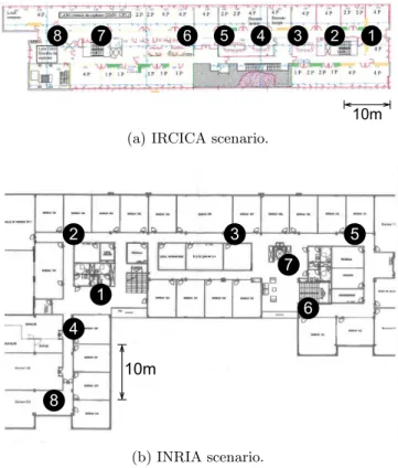
We have conducted experiments in two scenarios. We call the first one IRCICA, as we deployed our monitors at the second floor of the IRCICA/LIFL computer science labora-tory of Lille; and the second one INRIA as we conducted our experiments at the INRIA National Institute for Research in Computer Science and Control building also in Lille. Fig-ure 1(a) shows the placement of monitors along the corridor at IRCICA (leading to a linear shape). Note that moni-tors 1 to 6 are equally spaced, while monimoni-tors 7 and 8 are slightly separated from the others. At INRIA, as shown in

! " # $ % & ' ( !)*

(a) IRCICA scenario.

!"# ! $ % & ' ( ) * (b) INRIA scenario.

Figure 1: Monitor deployment for both scenarios.

Figure 1(b), monitors are placed along the L-shaped floor. Monitors cannot directly view each other, as they are sepa-rated by walls.

In both scenarios, the monitors sniffed the wireless net-work activity during 100 minutes, collecting IEEE 802.11b/g frames. Each monitor produced only one trace, listening to channel 1. The traces have an average size of 205 and 110 MByte at IRCICA and INRIA scenarios, respectively. In our experiments, each frame is limited to 220 bytes and the MAC addresses are anonymous.

Frame losses always occur independent from the sniffer hardware and software configuration [11]. In our experi-ments, we use Asus EEEPC-4G netbooks as sniffers. They are equipped with 512-MByte RAM and three USB Wi-Fi Netgear WG111v3 cards as wireless network adapters. The operating system is a Xandros OS with a customized kernel.

3. TRACE SIMILARITY

Hereinafter, we denote T = {t0, . . . , tn} the set of traces

captured in the same time period, where ti is the trace

collected by monitor si. We consider that each trace is

composed of flows of frames. We denote by fm

i the m

th

source-destination flow in trace ti and pni the nth frame in

ti. We denote the cardinality of a set by | • |.

We propose two metrics to discover how similar two traces are. The intra-flow similarity computes the ratio of the number of frames simultaneously captured by two given mon-itors nodes over the total number of frames captured by them. The inter-flow similarity, on the other hand, consid-ers the intconsid-ersection of flows instead of frames. Therefore, it is proportional to the ratio between the number of flows “ob-served” by the two monitors over the total number of flows

(4)

“observed” by them. A flow is considered “observed” if at least one of its frames is captured. In addition, since flows can have different numbers of frames, we give them different weights; the larger the number of frames in a flow, the more important it is.

3.1 Intra-flow similarity

We use the Jaccard similarity index to compute the intra-flow similarity. This metric considers all the frames captured by two sniffers, digging into each source-destination flow. This is why we consider this metric as intra-flow. Con-sidering two captured traces ti and tj as a set of frames,

ti= {p0i, . . . , pni}, the Jaccard similarity is:

J(ti, tj) = |ti∩ tj|

|ti∪ tj|· (1)

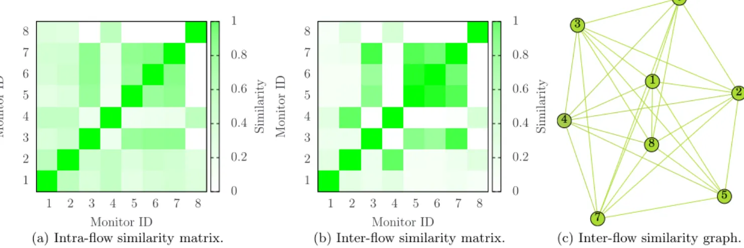
Figure 2(a) depicts the intra-flow similarity matrix of the traces from IRCICA. Each point (i, j) is gradually colored according to its value of J(ti, tj). As the monitors have been

sequentially placed, higher values are on the diagonal. In the figure, we can identify three geographical regions: a central region (monitors 4-5-6) and two side regions (monitors 1-2-3 and 7-8). As monitors 7-8 are slightly isolated from the oth-ers (see Figure 1(a)), they present a high similarity between them and low similarity with all the others. This means that small changes in monitors’ geographical placement have a big impact on the amount of original data captured. In the INRIA scenario, shown in Figure 3(a), traces 1 and 2 share a low intra-flow similarity with all the others and the remaining traces are split into two sets, 3-5-6-7 and 4-8.

3.2 Inter-flow similarity

From a higher point of view, it is worth considering the flows in common between two traces. The importance of each flow is proportional to the number of frames it has. Let us consider T the corpus of traces and each unique flow fm i

as a single term in a trace ti. We weight the importance of

the flow using the Term Frequency-Inverse Document Fre-quency (TF-IDF) metric [10]. TF-IDF is widely used in the information retrieval and text mining field to weight the similarity between two text documents. In our context, documents are traces and terms are flows. The inter-flow similarity between two traces ti and tj is computed as

fol-lows. If the union of the two traces has l distinct flows, a TF-IDF vector of l elements is assigned to each trace. Each element of the vector is the product of two factors. The first one is the flow frequency in that trace. The second one is the logarithm of the inverse trace (the one containing that flow) frequency over all the traces in the corpus.

TF-IDF(ti, l) = |fl i∪j| |ti| · log |T | |{ti∈ T |fi∪jl ∈ ti}| · (2)

The inter-flow similarity (IFS) is a value in the range [0;1] (from orthogonal traces to equal traces), given by the cosine of the angle between these vectors. This is equal to the dot product of the vectors, divided by the product of their magnitude: IFS(ti, tj) = P lTF-IDF(ti, l) · TF-IDF(tj, l) pP lTF-IDF(ti, l)2·pPlTF-IDF(tj, l)2 · (3)

In Figures 2(b) and 3(b), we can observe how the inter-flow similarity metric can clarify the relationship between traces. In the IRCICA scenario, Figure 2(b), we can clearly distinguish a first cluster of high similarity traces from mon-itors 7-8, which correspond to the monmon-itors located on the west side of the building. Because they are slightly separated from the other monitors, they present low similarity. Cen-tral monitors 4-5-6 compose another cluster, while on the east side of the building, we have a set of monitors 2-3 and a singleton with monitor 1. This last monitor produces a trace with a perceptible similarity with trace 2 fading down up to trace 6. We remark that, even if very geographically close, trace pairs 1-2 and 3-4 do not present a very high similarity among them.

Figure 3(b) shows that the traces from monitors 3-5-6-7, placed in the east side of the INRIA building (Figure 1(b)), have a very high inter-flow similarity as well as traces from monitors 2-4. Monitors 1 and 8 constitute two singletons.

4. MERGING EFFICIENCY

Deploying a large-scale WLAN monitoring system raises two important issues. First, deployment cost can be sig-nificant depending on the number of monitors. Second, it has a direct consequence on the amount of data to be post-processed. Moving such a bulk of data is an additional short-coming, since it impacts on the underlying network. There is then a tradeoff to respect between representativeness and scale.

Merging traces from different monitors is based on the assumption that a monitor might capture an event that an-other monitor misses. Merging together many traces, how-ever, is a CPU- and time-consuming process. The proce-dure is recursive and uses pairs of traces as input – with n traces, it would require n − 1 steps to synchronize, merge, and rewrite the final trace. Moreover, depending on the se-quence of traces to merge, this procedure converges faster or slower as similar traces (i.e., traces with several equal frames) do not contribute with unique frames when merged together. To tackle this issue, we propose a method to bet-ter chose the sequence of traces to merge. At the end, we show that the procedure improves system scalability without losing monitoring information.

4.1 Trace selection strategy

We consider the matrix of inter-frame similarity (IFS) values calculated in Section 3.2 and shown in Figures 2(b) and 3(b) as an adjacent matrix of a fully connected graph G(V, E). In this graph, each vertex vi corresponds to a

captured trace ti and each edge eij has a weight linearly

proportional to the IFS between traces tiand tj connected

(IFS(ti, tj)). For the sake of visualization, we consider the

length of each edge as proportional to its weight. We then use the Force Atlas algorithm embedded in the Gephi graph visualization and manipulation software to plot the graph [2]. Figures 2(c) and 2(c) show how nodes are arranged on a plane.

We observe that pairs of vertices with high similarity are likely placed farther away, whereas vertices with lower simi-larity are placed closer. Our hypothesis is that, touching all the nodes according to the minimum Hamiltonian path, is a smarter way to iteratively select traces to merge because it ranks the traces according to their contribution to the final merge. This rank is obtained from the path sequence, which

(5)

1 2 3 4 5 6 7 8 1 2 3 4 5 6 7 8 M o n it o r ID Monitor ID 0 0.2 0.4 0.6 0.8 1 S im il a ri ty

(a) Intra-flow similarity matrix.

(b) Inter-flow similarity matrix.

1 2 3 4 5 6 7 8

(c) Inter-flow similarity graph. Figure 2: IRCICA scenario. (a) and (b) are, respectively, the intra- and inter-flow similarity matrices between traces, whereas (c) is the graph generated using traces as nodes and inter-flow similarity values as edge lengths. 1 2 3 4 5 6 7 8 1 2 3 4 5 6 7 8 M o n it o r ID Monitor ID 0 0.2 0.4 0.6 0.8 1 S im il a ri ty

(a) Intra-flow similarity matrix.

(b) Inter-flow similarity matrix.

1 2 3 4 5 6 7 8

(c) Inter-flow similarity graph. Figure 3: INRIA scenario. (a) and (b) are, respectively, the intra- and inter-flow similarity matrices between traces, whereas (c) is the graph generated using traces as nodes and inter-flow similarity values as edge lengths.

is the solution of the Hamiltonian path problem. Traces at the beginning of the path contribute more to the merge in terms of number of unique frames, whereas traces at the end give a not relevant contribution. The full connectivity guar-antees the existence of such a Hamiltonian path. We refer to Hamiltonian path or Hamiltonian sequence equivalently. At the end of the procedure, we can select a subset of traces with higher contribution to be merged and we can also identify the monitors not satisfactorily contributing to the system. Merging a subset of traces can improve the sys-tem scalability while moving nodes to other points where they can have a higher contribution can enlarge the moni-tored area. We calculate the optimal Hamiltonian path with Concorde TSP Solver [6].

4.2 Evaluation

We evaluate our ranking strategy comparing its perfor-mance with a sequential strategy. As a sequential strategy, we mean merging the traces starting from monitor 1 and monitor 2 until monitor 8. We use this sequence because, as far as we know, there is no other work proposing a

dif-ferent method in the literature. Hence, we assume that the sequence is randomly chosen. For comparison purposes, we find the minimum Hamiltonian path starting from the trace captured by monitor 1 in both scenarios. It is worth men-tioning that the utilization of a different method was consid-ered such as using the trace size or the amount of frames per trace, but the differences among them are not appreciable.

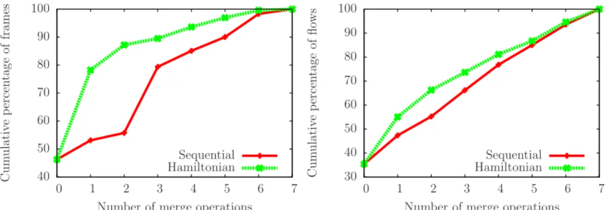
For the IRCICA scenario we get the Hamiltonian path 1-5-8-2-4-7-6-3. In Figure 4(a), we can appreciate how fast this sequence converges to the total covering of unique captured frames. We show the percentage of unique frames added to the final trace per merge procedure. As the first merge, the Hamiltonian sequence chooses trace 5 instead of trace 2, resulting in a positive percentage difference of 25% compared with the sequential strategy. At the second merge, the difference between trace 8 and 3, raises to 32%. From the third merge operation on the gap starts reducing. The Hamiltonian curve remains always on the top of the sequen-tial one, proving the importance of the right trace selection at the beginning of the whole merging process. Indeed, the first three chosen traces, 1-5-8, geographically cover all the

(6)

40 50 60 70 80 90 100 0 1 2 3 4 5 6 7 C u m u la ti v e p er cen ta g e o f fr a m es

Number of merge operations Sequential Hamiltonian

(a) New unique frames found over number of merge operations. 30 40 50 60 70 80 90 100 0 1 2 3 4 5 6 7 C u m u la ti v e p er cen ta g e o f fl o w s

(b) New unique flows found over number of merge operations.

Figure 4: IRCICA scenario. Comparison between the Hamiltonian merging sequence (1-5-8-2-4-7-6-3) and the sequential merging order.

40 50 60 70 80 90 100 0 1 2 3 4 5 6 7 C u m u la ti v e p er cen ta g e o f fr a m es

(a) New unique frames found over number of merge operations. 30 40 50 60 70 80 90 100 0 1 2 3 4 5 6 7 C u m u la ti v e p er cen ta g e o f fl o w s

(b) New unique flows found over number of merge operations.

Figure 5: INRIA scenario. Comparison between the Hamiltonian merging sequence (1-6-3-4-7-8-5-2) and the sequential merging order.

area and 87% of all the captured frames. In addition, if the traces merged at steps 3-4-5-6 can still add a small amount of new frames, the last merged trace (trace 3) does not gen-erate a significant increment. This suggests that its utiliza-tion is not relevant and could be left aside or it suggests that monitor 3 should be better moved somewhere else.

Regarding the quantity of unique flows detected, the Hamil-tonian selection strategy presents a faster covering. Fig-ure 4(b) shows the percentage of unique flows added to the final trace per merge procedure. The largest differences com-pared with the sequential strategy are at the firsts merging steps: 9% higher at the first step and 11% higher at the second. Comparing Figures 4(a) and 4(b), we also remark that flows chosen at the beginning are the most significant ones contributing with a large number of frames. From the third merging step on, 27% of new flows are detected with only 12% of new unique frames.

The INRIA scenario also shows that the Hamiltonian strat-egy leads to a better performance compared with the sequen-tial one, even when monitors are not geographically placed respecting the sequential order. In this case, the trace se-quence given by the Hamiltonian path is 1-6-3-4-7-8-5-2.

Figure 5(a) shows the performance of the Hamiltonian strat-egy in INRIA scenario. Again, the largest difference appears at the first steps. Choosing to merge traces 1 and 6, instead of 1 and 2, we have an increment of 22% in the percentage of unique frames captured. We also note that, choosing the Hamiltonian sequence, the last two monitors, do not pro-duce a significant improvement. These monitors could be better moved somewhere else to enlarge the monitored area without a significant loss.

Figure 5(b) shows that even considering steps 5 and 6, where the sequential procedure detects more flows, the Hamil-tonian strategy still detects more unique frames. The se-quential strategy detects more flows in these steps because most frames are merged at the very beginning of the whole procedure.

5. SUMMARY AND OUTLOOK

In this work we show how to better scale current monitor-ing systems, selectmonitor-ing the monitors which produce the most significant contribution for the merging procedure. Starting from a set of captured traces, we first compute the inter-flow similarity between all of them. Then, we model the

(7)

network as a graph to find the most appropriate sequence of merges. This sequence is found using the minimum Hamil-tonian path, computed on such graph, which sorts the traces according to their contribution to the final merged file. Our approach leads to two main improvements. The system can become more scalable, since the merges can be limited to a subset of traces at the beginning of the sequence; and the system can become larger, since last traces in the sequence can suggest moving the monitors to other areas.

Although the inter-flow similarity looks like to have a good impact on the trace selection, we wish to exploit other sim-ilarity metrics. We used the optimum Hamiltonian path starting from trace 1 in order to compare it with a sequen-tial merging. A further improvement could be the utilization of the absolute minimum path.

Acknowledgments

Matteo Sammarco and Marcelo Dias de Amorim carried out part of the work at LINCS (http://www.lincs.fr). Miguel Campista would like to thank CAPES, CNPq, FAPERJ, and FINEP for their support. This work was partially funded by the French National Research Agency (ANR) under the project ANR VERSO RESCUE (ANR-10-VERS-003).

6. REFERENCES

[1] A. Balachandran, G. M. Voelker, P. Bahl, and P. V. Rangan. Characterizing user behavior and network performance in a public wireless LAN. In ACM SIGMETRICS, pages 195–205, June15-19 2002. [2] M. Bastian, S. Heymann, and M. Jacomy. Gephi: an

open source software for exploring and manipulating networks. 2009. In International AAAI Conference on Weblogs and Social Media, 2011.

[3] Y.-C. Cheng, J. Bellardo, P. Benk¨o, A. C. Snoeren, G. M. Voelker, and S. Savage. Jigsaw: solving the puzzle of enterprise 802.11 analysis. In ACM SIGCOMM, pages 39–50, Sept.11-15 2006. [4] T. Claveirole and M. D. de Amorim. WiPal: IEEE

802.11 traces manipulation software, Jan. 2010.

[5] T. Claveirole and M. D. de Amorim. Manipulating Wi-Fi packet traces with WiPal: design and experience. Software Practice & Experience, 42(5):585–599, May 2012.

[6] W. Cook. Concorde TSP solver. See: http://www. tsp. gatech. edu/concorde. html, 2005.

[7] T. Henderson, D. Kotz, and I. Abyzov. The changing usage of a mature campus-wide wireless network. In ACM MobiCom, pages 187–201, Sep.-Oct.26-1 2004. [8] C. C. Ho, K. N. Ramachandran, K. C. Almeroth, and

E. M. Belding-Royer. A scalable framework for wireless network monitoring. In Proceedings of the 2nd ACM international workshop on Wireless mobile applications and services on WLAN hotspots, WMASH ’04, pages 93–101, New York, NY, USA, 2004. ACM. [9] R. Mahajan, M. Rodrig, D. Wetherall, and

J. Zahorjan. Analyzing the MAC-level behavior of wireless networks in the wild. In ACM SIGCOMM, pages 75–86, Sept.11-15 2006.

[10] J. Ramos. Using TF-IDF to determine word relevance in document queries. In Proceedings of the First Instructional Conference on Machine Learning, 2003. [11] P. Serrano, M. Zink, and J. Kurose. Assessing the

Fidelity of COTS 802.11 Sniffers. In INFOCOM 2009, IEEE, pages 1089–1097, April.

[12] Y. Sheng, G. Chen, H. Yin, K. Tan, U. Deshpande, B. Vance, D. Kotz, A. Campbell, C. McDonald, T. Henderson, and J. Wright. MAP: a scalable monitoring system for dependable 802.11 wireless networks. Wireless Communications, IEEE, 15(5):10–18, October.

[13] K. Tan, C. McDonald, B. Vance, C. Arackaparambil, S. Bratus, and D. Kotz. From MAP to DIST: the evolution of a large-scale WLAN monitoring system. IEEE Transactions on Mobile Computing,

99(PrePrints):1, 2012.

[14] J. Yeo, M. Youssef, and A. Agrawala. A framework for wireless lan monitoring and its applications, 2004.