1
2
3
An early forest inventory indicates a high accuracy of forest composition data in 4
presettlement land surveys records 5
6
Terrail R. 1,4, Arseneault D.1*, Fortin M.-J.2, Dupuis S. 1,5 & Boucher Y. 3 7
8
9
10
11
1: Groupe BOREAS, Centre d'études nordiques and Chaire de Recherche sur la Forêt Habitée 12
Université du Québec à Rimouski, 300 Allée des Ursulines, Rimouski (Québec), Canada, G5L 3A1; 13
2: Department of Ecology & Evolutionary Biology, University of Toronto, 25 Harbord Street, Toronto 14
(Ontario), Canada, M5S 3G5; mariejosee.fortin@utoronto.ca 15
3: Direction de la recherche forestière, Ministère des Ressources naturelles, 2700, Einstein, Québec 16
(Québec), G1P 3W8, Canada; Yan.Boucher@mrn.gouv.qc.ca 17
4:titeraph@gmail.com 18
5:sebastien_dupuis@uqar.ca 19
*Corresponding author; phone: 418-723-1986 ext. 1519, fax: 418-723-1849; 20 dominique_arseneault@uqar.ca 21 22 23 24
ABSTRACT 25
Questions: Do early land survey records of the "line description" type allow accurate 26
reconstructions of presettlement forest composition? Did surveyors record all tree taxa in forest 27
stands encountered along the surveyed lines? Were taxa ranked according to their relative 28
importance in forest stands? What criteria did surveyors used to rank taxa in stands? 29
Location: Northern range limit of northern hardwoods in the Lower St. Lawrence region of 30
eastern Québec, Canada. 31
Methods: Validation of 1695 taxa lists recorded by surveyors in the 19th century by comparison 32
with the number of stems by tree species and stem diameter classes recorded in 2790 old growth 33
plots over the same two regions during a 1930 forest inventory. 34
Results: Taxon prevalence and dominance (i.e. proportion of observations for which each taxon 35
is dominant) are highly correlated between the presettlement surveyors and the 1930 forest 36
inventory data sets. Surveyors ranked taxa by decreasing order of relative importance, using 37
criteria directly equivalent to basal area of stems in modern forest inventory plots. Taxon 38
prevalence is more accurately reconstructed using relative metrics (i.e., ranks of taxon prevalence 39
in region), whereas taxon dominance is more accurately reconstructed using absolute metrics 40
(percent of stands dominated across landscapes). The early land surveys allow the spatial patterns 41
of forest composition to be reconstructed by computing relative taxa prevalence in cells of 3 km 42
x 3 km. Prevalence of balsam fir (Abies balsamea) and white birch (Betula papyrifera) are 43
underestimated in surveyors data, probably reflecting their low economic value during the 19th 44
century. 45
Conclusions: Taxon lists of early surveyors can accurately reconstruct presettlement forest 46
composition and spatial patterns by using metrics of taxa prevalence and dominance across 47
landscapes. Relative prevalence is a more comprehensive description of forest composition than 48
dominance, but tend to underestimate some taxa. Absolute taxon dominance is a more robust 49
metric than prevalence, but only reports on the abundance of the most dominant taxa. 50
51
KEWORDS: Early land survey records, Historical forest ecology, Line descriptions, Northern 52
hardwoods, Presettlement forest composition, Taxa prevalence, Taxa dominance 53
NOMENCLATURE: Farrar (1995) 54
ABBREVIATIONS: LDs: line descriptions 55
RUNNING HEAD: Forest composition from land survey archives 56
57
INTRODUCTION 58
North American forest ecosystems have experienced important and rapid compositional 59
changes since European settlement, especially in the densely settled temperate zone 60
(Whitney1994; Thompson et al 2013). Early land survey records have been widely used to 61
reconstruct these changes (Lorimer 1977; Foster et al 1998; Jackson et al. 2000; Rhemtulla et al. 62
2007). Surveyors mandated to divide the public lands prior to settlement described the forest 63
composition along the surveyed lines in their notebooks. As large regions were systematically 64
surveyed, these data allow the reconstruction of large-scale vegetation patterns from several 65
thousand, spatially precise, in situ observations of forest composition (Cogbill 2002; Friedman & 66
Reich 2005; Rhemtulla et al. 2007), and provide historical forest baselines for forest 67
management, biodiversity conservation, and restoration efforts (Landres et al. 1999; Foster et al. 68
2003; Rhemtulla et al. 2009). 69
Two main types of forest composition data exist in land survey records in North America. 70
The type most often used consists of the description (species, diameter, angle, and distance to 71
post) of a few individual witness trees (generally 2-4 stems) selected by surveyors around posts, 72
which were distributed over a half-mile grid. This type of data is mainly associated with the 73
survey regime implemented by the General Land Office (GLO) from 1812 onward, notably in the 74
American Midwest (Whitney 1994). The second type consists of descriptive accounts in the form 75
of ranked taxon lists along survey lines (Jackson et al. 2000; Scull & Richardson 2007; Fritschle 76
2009). These line descriptions (hereafter LDs) have been much less often used to reconstruct 77
historical forest compositions, probably because they frequently represent the average forest 78
composition over one-mile long (1.6 km) line segments (Whitney & DeCant 2001). However, in 79
eastern Canada, LDs are generally the only land survey type systematically available (Gentilcore 80
& Donkin 1973; Clarke & Finnegan 1984; Jackson et al. 2000; Crossland 2006; Pinto et al. 2008) 81
and were generally made over much shorter line segments than under the GLO regime, and thus 82
The reconstruction of postsettlement compositional changes has been achieved primarily by 84
comparing modern forest inventories with either witness tree or LD archive data. The modern 85
inventories are generally based on dense networks of plots in which stem density is described in 86
species and stem diameter classes. Such comparisons between time periods assume that datasets 87
constructed from early land surveys and modern plots are unbiased descriptors of the forest 88
composition and that they can be compared in spite of their contrasting nature. 89
Several analyses of archive "witness trees" type surveys have been done to quantify bias in 90
data and verify robustness of forest reconstructions. Most validation studies were performed by 91
comparing data subsets thought to be differently biased (Manies & Mladenoff 2001; Liu et al. 92
2011). Surveyed sites have also been resampled, but to a limited scale due to the rarity of 93
unaltered landscapes (Manies & Mladenoff 2000; Williams & Baker 2010). Overall, these studies 94
have shown that witness trees allow robust reconstructions of presettlement forest composition 95
and structure. However, biases arising from surveyor preferences are present. Surveyors 96
consistently selected against both small and large trees, in favor of trees closer to posts and in 97
favor of some species features such as a low bark roughness of trees to be blazed (Bourdo 1956, 98
Manies et al 2001; Schulte & Mladenoff 2001; Liu et al.2011). As a result, measures of relative 99
taxa abundance are generally less biased than measures of absolute abundance and reconstruction 100
of forest composition in large regions are more robust than reconstruction at local scales (Schulte 101
& Mladenoff 2001; Liu et al.2011, Williams & Baker 2011). 102
To our knowledge, land survey records of the LD type have never been assessed for bias, 103
despite potential problems arising from the particular nature of these data. We do not know if all 104
taxa were listed in all stands along the surveyed lines. In addition, although taxa were probably 105
listed in decreasing order of importance, as suggested by the frequent inversion of taxa between 106
consecutive lists, criteria used to rank taxa importance are unknown. We also do not know how 107
these potential problems propagate from the stand scale to the larger scales of landscapes and 108
regions at which reconstructions of presettlement forest composition are generally performed. 109
In the Lower St-Lawrence region of eastern Canada, the Price Brother's Company 110
performed a forest inventory based on a dense plot network (hereafter referred to as the "early 111
forest inventory") between 1928 and 1930. Similarly to modern forest inventories, tree stems 112
were then counted according to species and diameter classes in several thousand, precisely 113
located plots. A subset of these plots overlapped several LDs that had previously been made 114
between 1860 and 1900, thus offering the opportunity to validate LD using a completely 115
independent, quantitative dataset. The objective of our study is thus to verify if LDs can be used 116
to reconstruct presettlement forest composition. In particular, we verify if taxon prevalence and 117
dominance (i.e., the percent of observations for which a taxon is ranked first by surveyors) are 118
correlated between the LD survey and the early forest inventory. We also verify if all taxa were 119
listed in taxon lists, if taxon were ranked in decreasing order of importance in stands, and if 120
surveyors determined taxa importance based on stems density or volume (i.e. basal area) in 121
stands. An additional objective is to evaluate if spatial patterns of presettlement species 122
abundance can be reconstructed from the LD survey. Because the early forest inventory is similar 123
to modern inventories, our results will help compare forest composition between the LD survey 124
and present-day data. 125
126
STUDY AREA 127
The study area is situated in the province of Québec in eastern Canada and lies between the 128
Saint Lawrence River to the north and the province of New Brunswick and the state of Maine 129
(USA) to the south. It is located at the northern limit of the Great Lakes–Saint Lawrence forest 130
region (Rowe 1972). This area belongs to the Appalachian geological formation, which is 131
characterized by sedimentary bedrock and is covered by surficial deposits of alteration and 132
glacial origins (Robitaille & Saucier 1998). The topography consists of low elevation hills that 133
gradually increase in altitude to reach just below 500 m towards the southwest and just below 134
900 m towards the northeast. Climate conditions can be portrayed from the weather stations of 135
Rimouski and Matane (Fig. 1). The mean annual temperature varies between 2.7 and 3.9 °C (-14 136
to -11.7 °C in January and 17.9 to 18.2 °C in July), with mean annual precipitations reaching 915 137
to 1202mm, of which 24% to 36 % falls as snow (Environment Canada 2013). 138
The study area comprises two distinct regions, Matane and Rimouski, in which the 1930 139
early forest inventory overlapped the previous LD surveys (Fig. 1). The Matane region covers an 140
area of 315 km2 between 67°40’ and 66°50’ W longitude, and 49° 00' and 48°30’ N latitude. 141
According to the Québec Government’s forest site classification system (Grondin et al. 1998), 142
mesic sites are typically characterized by mixed stands of balsam fir (Abies balsamea), white 143
spruce (Picea glauca), and white birch (Betula papyrifera). Black spruce (Picea mariana), and 144
aspen (Populus tremuloides) occur locally. The Rimouski region is located 80 km to the 145
southwest of the Matane region (Fig. 1) and covers an area of 378 km2, between longitudes 68° 146
00' to 68°50' W and latitudes 47°50' to 48°30' N. Mesic sites are dominated by balsam fir, yellow 147
birch (Betula alleghanensis), white birch, and aspen. Sugar maple (Acer saccharum) and red 148
maple (Acer rubrum) are generally dominant on upper slopes and hill tops below 500 m in 149
elevation. Eastern white cedar (Thuya occidentalis) frequently dominates on organic soils and 150
within riparian forests along streams and lakeshores. 151
152
MATERIAL AND METHODS 153
Field notes of the early forest inventory and maps of the corresponding transect lines are 154
contained in the Price fonds of Québec national archives in the town of Chicoutimi. The Price 155
Brother's Company conducted the inventory between 1928 and 1930 in order to evaluate the 156
available wood volume on its timber limits. Plots of 1012 m2 (5 chains by 0.5 chains; 1 chain = 157
20.12 m) were spaced by about 100 m to 300 m (5 to 15 chains) along transects, which were 158
themselves spaced by 120 m to 1700 m. Mean plot density was 6.4 and 2.1 plots per km2 at 159
Matane and Rimouski, respectively (Fig. 1). Stems were classified by species and 2 inch (5.1 cm) 160
DBH (diameter at breast height) classes at each plot, with a minimum of 3 inches (7.6 cm). 161
Because of the very high plot density and their systematic location (Fig. 1), we assume that the 162
early forest inventory portrays an unbiased forest composition. In addition, as most forest stands 163
in this area were old-aged in 1930 (Boucher et al. 2009a), we assume that their composition 164
remained relatively stable between the time period of the LD survey (1859-1900) and the early 165
forest inventory in 1930. 166
According to the survey regime that prevailed in the province of Québec, townships of 167
about 15 km x 15 km were subdivided into parallel, 1-mile wide (1.6 km) ranges. LDs were 168
conducted along range lines and township boundaries and included the precise measurement of 169
distances between successive observations. Various observations on forest composition can 170
generally be found in the surveyor's notebooks, such as taxon lists (e.g. spruce, fir, birch, cedar, 171
and a few maple) and specific cover types (e.g. maple stand, cedar stand, etc.). In this study, 172
specific cover types were considered equivalent to pure stands of the corresponding taxa. General 173
cover types (e.g. mixed wood, hardwood) and mentions of recent disturbances (fire, logging, 174
wind throw) are also frequent, but were not considered in this study. All retained LD 175
observations were georeferenced using ARCGIS 10 (ESRI 2011) over a governmental cadastral 176
map built from early land surveys (Dupuis et al. 2011). 177
We adjusted the two datasets to make them comparable. In total, 729 and 966 taxon lists 178
were available, compared to 2013 and 777 early inventory plots for the Matane and Rimouski 179
region, respectively. Because the resolution of taxa (i.e. species vs. genera) varied between the 180
two datasets, spruce (white, black, and red spruce), maples (sugar and red maple), pines (red, 181
white, and jack pine) and poplars (aspen and balsam poplar) were grouped to the genera level 182
within the two datasets. Taxa mentioned in less than 4% of taxon lists (ash, larch, elm, alder, 183
mountain ash, etc.) were grouped as "others". Balsam fir and eastern white cedar were considered 184
at the species level, as only one species is present in the region for these two genera. Similarly 185
white and yellow birches were considered at the species level, as surveyors systematically 186
distinguished these two taxa. Hence, although taxa grouping would tend to increase the similarity 187
of the two datasets, the most prevalent taxa (fir, cedar and white birch, see results), except spruce, 188
could be considered at the species level. The grouping of spruces and maples species to the 189
genera level is an intrinsic limitation of these LD data (Dupuis et al 2011). 190
Stand age and the occurrence of previous logging were evaluated in the field for each plot 191
during the 1930 forest inventory. Consequently, all plots previously logged and plots less than 80 192
years old in 1930 could be excluded from all analyses to avoid forest stands that were severely 193
disturbed between the LD survey and the forest inventory. In addition, we considered only forest 194
inventory plots situated at less than 1 mile (1.6 km) from a range line of the LD survey, as this 195
distance separates range lines in the LD survey. Because LDs provide taxon lists, presumably 196
ranked according to taxon importance in stands, comparable taxon lists were constructed for each 197
early forest inventory plot. As we did not know a priori the criteria used by surveyors to rank 198
taxon in lists, two taxon lists were constructed separately for each plot, by ranking taxa according 199
to total stem density and total basal area, respectively. 200
Data analysis 201
In this study the prevalence of a taxon corresponds to its overall frequency and was 202
computed as the % of all observations containing each taxon, regardless of the ranking position 203
in the taxon lists, for each region and both datasets. We then regressed taxa prevalence in the 204
forest inventory plots against prevalence in LDs in order to verify if LDs allowed taxa prevalence 205
to be reconstructed across landscapes. In addition, we used a maximum likelihood test to verify 206
the null hypothesis that the regression line has a slope of one and that taxon prevalence is directly 207
proportional between the LD survey and the forest inventory. 208
To confirm that surveyors ranked taxa in lists, we calculated taxon frequency at each 209
position in the lists using the formula (Scull & Richardson 2007): 210
Fir = (Nir/Nr) x 100 (eq. 1) 211
where Nir is the number of times taxon i is ranked at position r in the taxon lists and Nr is
212
the total number of lists containing taxon i. For the early forest inventory, Fir has been computed
213
two times, with taxa ranked according to total basal area and total stem density, respectively. 214
Then, for each region and each taxon, distributions of taxon frequency at each ranking position 215
were compared between LD and the forest inventory plots using a Kolmogorov-Smirnov test. In 216
this analysis, we considered only taxa with a prevalence equal or greater than 20% in the two 217
datasets at Matane (balsam fir, spruce, cedar, and white birch) and Rimouski (balsam fir, spruce, 218
cedar, white birch, and yellow birch). 219
The frequency of a taxon at the first ranking position (i.e., for r = 1 in eq. 1) is hereafter 220
referred to as taxon dominance. As for taxon prevalence, we verified if taxon dominance is 221
correlated between both datasets and if the corresponding regression slope is significantly 222
different from 1. Dominance was first log-transformed because of its non-normal distribution. 223
We used an index of co-occurrence, Cij, to compare taxa assemblages between the LD
224
survey and the forest inventory, using the following formula: 225
Cij= Lij/Lj (eq.2)
226
where Lij is the number of taxon lists with taxon i when taxon j is ranked first and Lj is the
227
number of lists with more than one taxa and having taxon j ranked first (Dupuis et al. 2011). 228
229
Absolute vs. relative metrics 230
Previous studies have concluded that relative measures of forest structure and composition 231
(e.g. rank of taxon abundance) are generally more accurately reconstructed with GLO data than 232
absolute measures (e.g. absolute stem density or basal area) (Schulte & Mladenoff 2001; 233
Rhemtulla & Mladenoff 2009). Consequently, we have verified if relative taxon prevalence and 234
dominance are more similar between datasets than their absolute equivalents. Taxa were ranked 235
in decreasing order of prevalence and dominance over the entire Matane and Rimouski regions 236
and ranks were compared between the LD surveys and the forest inventories. Taxa with an 237
absolute prevalence of less than 5% were excluded from this analysis because of insufficient 238
data. 239
We have also compared spatial patterns of taxon prevalence between datasets. The Matane 240
and Rimouski regions were divided into cells of 3 km x 3 km. Cells with less than 5 taxon lists 241
and less than 5 forest inventory plots were excluded. The remaining cells contained an average of 242
21 and 23 taxon lists compared to 57 and 24 forest inventory plots in the Matane and Rimouski 243
region, respectively. As the two datasets were more similar for relative taxon prevalence than for 244
alternative metrics (Table 1; see results), we calculated the relative prevalence of each taxon for 245
each cell of each region. Subtracting the relative taxon prevalence between the LD survey and the 246
forest inventory allowed differences between datasets to be assessed on a cell-by-cell basis. 247
Frequency distributions of prevalence differences between the LD survey and the forest 248
inventory were then compiled to verify that the modal difference was close to zero. 249
250
RESULTS 251
LD surveys allow accurate reconstructions of presetttlement forest composition. 252
Considering both regions together, taxon prevalence is highly correlated between the LD survey 253
and the early forest inventory (Table 1 and Fig. 2a; r = 0.97; p < 0.0001; n = 18). This high 254
similarity between the two independent datasets implies that surveyors frequently listed all taxa 255
in the forest stands encountered on the range lines. Balsam fir, spruce, and white birch were the 256
most prevalent taxa in both regions and datasets, with prevalences greater than 75%, except for 257
white birch in the LD survey at Rimouski (prevalence of 50%). Cedar and yellow birch exhibited 258
intermediate prevalences of 15%-50% in both datasets and regions. The most important 259
differences between regions were similar in both datasets and reflect the greater prevalence of 260
cedar, maple, and poplar at Rimouski than at Matane. The LD survey also allows for the direct 261
reconstruction of the absolute prevalence of most taxa, as we cannot reject the null hypothesis of 262
a regression slope of 1 between the LD survey and the early forest inventory (maximum 263
likelihood test; p = 0.069; df = 17). However, lower prevalence values, by 20%-30% in the LD 264
survey, as compared to the early forest inventory for balsam fir, white birch, and yellow birch at 265
Rimouski, suggests that surveyors did not always list these three taxa when they were present in 266
the field. The biases against balsam fir and white birch at Rimouski were generalized, as 267
indicated by their co-occurrence indices that are at least 10% lower for the LD survey as 268
compared to the early forest inventory (Appendices S1 and S2 in supporting information). 269
The LD survey also allows accurate reconstruction of taxon dominance in the presettlement 270
forest. Taxon dominance is highly correlated between the two datasets, considering that either 271
total basal area (r = 0.93; p < 0.0001; n = 18) or stem density (r = 0.85; p < 0.0001; n = 18) were 272
used to rank taxa in plots of the early forest survey (Fig. 2b, c). However, in contrast to stem 273
density (regression slope significantly different from 1; p=0.03; df = 10), basal area in plots 274
(slope not significantly different from 1; p=0,13; df=14) is a direct indicator of taxa dominance in 275
the LD survey. When taxon dominance in the forest inventory is based on stem density, the LD 276
survey underestimates the dominance of balsam fir, a taxa that occurred at very high stem 277
densities in the inventory plots of the two regions. Conversely, for the remaining taxa that 278
occurred at lower densities than balsam fir, taxon dominance in the LD survey overestimates 279
dominance based on stem density in the early forest inventory (Fig. 2c). 280
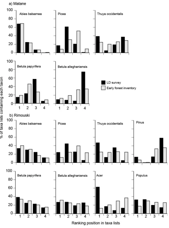
Rank positions in taxon lists of the LD survey are more similar to rank based on basal area 281
than ranks based on stem densities in plots of the early forest inventory. Considering the basal 282
area of taxa, distributions of rank frequencies are not significantly different between the LD 283
survey and the early forest inventory (Kolmogorov-Smirnov test; p<0.05; Fig. 3), except for 284
cedar at Rimouski that tends to occur more frequently at the first ranking position in the LD 285
survey than in the early forest inventory. Although distributions of rank frequencies for spruce 286
are not significantly different between datasets, in both regions the modal frequency occur at the 287
second rank for the LD survey and at the third rank for the early forest inventory. Considering 288
stem density, distributions of rank frequencies are significantly different between the LD survey 289
and the early forest inventory for cedar and white birch in both regions and for spruce and yellow 290
birch at Rimouski (Kolmogorov-Smirnov test, p<0.05; Appendix S3). 291
Relative taxa prevalence appears to be the more robust metric of presettlement forest 292
composition in the LD survey. Ranks of taxa prevalence (i.e. relative prevalence) are similar in 293
the LD survey and the early forest inventory for both regions, except for balsam fir and spruce, 294
which are inverted between the first two ranking positions at Rimouski (Table 1). In contrast, 295
relative dominance, either based on basal area or stem density in plots, is much less similar 296
between the two datasets. At Rimouski in particular, relative taxa dominance differs by at least 297
one ranking position between datasets, except for the dominance of spruce based on density 298
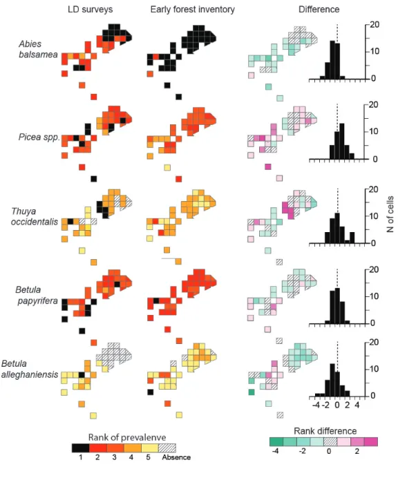
(Appendix S4). Relative taxa prevalence also allows for the mapping of presettlement forest 299
composition spatial patterns. Maps of relative taxa prevalence are similar between the LD survey 300
and the early forest inventory in both regions (Figs 4, 5). The frequency of differences in relative 301
prevalence on a cell-by-cell basis between the two maps is mostly symmetrical with a mode of 0, 302
-1, or 1. Only spruce at Matane (mode = -2) and white (-2) and yellow (+2) birch at Rimouski 303
deviate from this trend. 304
305
DISCUSSION 306
The early forest inventory made by the Price Brother's Company in 1928-30 allows forest 307
composition data in the LD survey to be compared and assessed using a high-quality, completely 308
independent data source. Similar to modern forest surveys, the early forest inventory included 309
the precise quantification of taxon abundance by stem diameter classes in a large number of 310
precisely delineated plots. These early plots were even larger (1000 m2 vs. 400 m2) and denser at 311
Rimouski (2.1 vs. 1.1 per km2) and Matane (6.4 vs. 0.77 per km2) than plots of the most recent 312
governmental forest survey, which was done in the 2000's. The early plots were also 313
systematically located on transect lines, covering the entire range of environmental conditions 314
likely to have influenced the presettlement forest composition. The overlaps of the LD survey 315
with the early forest inventory over two different regions with slightly different forest 316
compositions 80 km apart is another condition that contributed to the robust assessment of LD 317
forest composition data. 318
The time lag of 30 to 70 years between the LD surveys and the early forest inventory may 319
have biased the comparison of the two datasets, even if sites logged prior to 1930 were excluded 320
from the study. However, our results as well as previous studies (Boucher et al. 2009a; Dupuis et 321
al. 2011), have shown that severe disturbances were infrequent in the preindustrial forests of the 322
study area, which were dominated by late-successional, shade-tolerant or long-living tree species 323
(mostly fir, spruce and cedar), along with the less tolerant white birch. Outbreaks of the spruce 324
budworm (Choritoneura fumiferana [Clem.]) were probably the most important disturbances in 325
these preindustrial forests, recurring every 30 to 40 years (Boulanger and Arseneault 2004). As 326
the main hosts of the budworm, fir and spruce, also recover rapidly following outbreaks (Morin 327
1994), forest composition probably remained relatively stable in sites that had not been logged 328
prior to 1930. This assumption is supported by the similar forest composition between the two 329
datasets. 330
Our results indicate that LDs made during the early survey of public lands in eastern 331
Canada permit accurate reconstructions of presettlement forest composition using metrics of taxa 332
prevalence and dominance across landscapes. The very high correlations of taxon prevalence 333
and dominance between the LD survey and the early forest inventory demonstrate that the two 334
datasets are very similar in regard to these metrics and would have resulted in very similar 335
reconstructions of forest composition for the two studied regions. The high correlation of taxon 336
prevalence between the two datasets indicates that surveyors frequently listed all the most 337
important taxa present in stands. Likewise, similar taxon dominances between datasets, as well 338
as similar frequency distributions of ranking positions in taxon lists, clearly demonstrate that 339
surveyors ranked taxa according to their relative importance in stands, as previously supposed in 340
most studies based on LDs (Jackson et al. 2000; Scull & Richardson 2007; Pinto et al. 2008; 341
Dupuis et al. 2011). An important contribution of our study in this regard is the demonstration 342
that the ranking of taxa based on basal area in forest inventory plots is an unbiased estimator of 343
taxa ranks in taxon lists contained in the LD survey, especially for taxon dominance (i.e., for the 344
first ranking position). Surveyors most likely ranked taxa according to their visual importance in 345
stands, explaining why basal area, which is computed from both stem diameter and density, is a 346
better ranking variable than stem density alone. 347
However, biases are also present in the LD survey taxon lists. Because the prevalence of a 348
taxon corresponds to its frequency of occurrence amongst taxon lists, regular omissions of a 349
taxon by surveyors would have caused its prevalence to be significantly lesser in LDs as 350
compared to early inventory plots. While taxon prevalence is almost perfectly correlated 351
between datasets at Matane, prevalence of balsam fir, white birch, and yellow birch appears to 352
be underestimated by 20-30% in the LD survey at Rimouski. This problem reduced the co-353
occurrence of fir and white birch with other taxa and inverted the first two ranks of relative 354
prevalence between spruce and fir in the LD survey, as compared to the early forest inventory. 355
The specificity of the prevalence bias for the Rimouski region probably results from its more 356
diversified forest composition in comparison to the Matane region. 357
The prevalence bias against balsam fir may also be explained by its low economic 358
importance over the 19th century. Although fir was clearly the most prevalent taxon in both 359
regions, it had not been commercially exploited until the rise of the pulp and paper industry at 360
the beginning of the 20th century (Boucher et al. 2009a, b). An additional explanation is the low 361
stature of fir stems and their high shade tolerance (Kneeshaw et al. 2006). Plots of the early 362
forest inventory indicate that balsam fir frequently displayed a high density of low to mid-363
diameter stems with infrequent large trees. As surveyors considered the visual importance of 364
taxa in stands, they may have neglected balsam fir in stands where it occurred as small 365
suppressed trees. The remaining most prevalent taxa (spruce, cedar, yellow and white birch) 366
frequently comprised large stems that would have increased their visual importance relative to 367
balsam fir. The bias against white and yellow birch may also be associated with their low 368
economic value in the 19th century, as well as with the exclusion in this study of general cover 369
types mentioned by the surveyors. A previous study in the Rimouski region indicated that 370
"mixewood" was by far the most frequent cover type mentioned and that it included yellow and 371
white birch with prevalence of about 45 % - 65 % (Dupuis et al. 2011). 372
Conversely our study suggests no significant prevalence bias for eastern white cedar, 373
spruce, and pine. Overestimation of the prevalence of these taxa would have been likely, given 374
their important economic value and frequent large to very large stems in presettlement forests. 375
For example, the frequent mention by surveyors of "cedar stands" along streams may have been 376
considered as a positive bias, reflecting the high economic value of this taxon. In fact, it may be 377
that prevalence of these taxa is not significantly biased in the LD survey, specifically because 378
they received greater attention from the surveyors as compared to the less preferred taxa. If 379
surveyors listed the important taxa every time they where encountered, then their prevalence in 380
the LDs would precisely reflect the actual forest composition at the time of the surveys. Taxon 381
dominance also appears to be free of such biases because it depends only on the first ranked 382
position in the lists and the most dominant taxa in stands were probably easily identified in the 383
field. However, as dominance only provides data concerning the taxa that are dominating stands, 384
it is a less comprehensive metric of forest composition than taxon prevalence. 385
Relative taxon prevalence was shown to be an even better metric of taxon abundance than 386
absolute prevalence. Considering relative prevalence, the LD survey almost perfectly replicates 387
the early forest inventory, except for spruce and fir that are inverted between the first two 388
prevalence ranks at Rimouski. This strengthened similarity probably arises through the 389
considerable simplification of data complexity when values of absolute prevalence, which vary 390
between 0 % and 100 %, are condensed to a few discrete ranks. Such simplification reduces bias 391
that may have propagated in data from surveyor subjectivity when visually assessing the relative 392
importance of taxa in the field (Schulte & Mladenoff 2001). An additional contributing factor is 393
the regular distribution of absolute taxa prevalence within the range of possible values between 0 394
and 100 %. In contrast to prevalence, values of absolute dominance are mostly clustered below 395
30 %, making it difficult to clearly distinguish taxa based on their rank of relative dominance. As 396
presettlement temperate forests tended to be dominated by a few taxa out of the regional species 397
pool (Cogbill et al. 2002), dominance values of the various taxa will generally be more clustered 398
at lower values than taxon prevalence, suggesting that relative taxon dominance would rarely be 399
an appropriate metric to reconstruct forest composition from the LD survey. 400
LD surveys also allow the reconstruction of presettlement forest composition spatial 401
patterns. Even if public land survey records have been frequently used to reconstruct the spatial 402
variability of forest composition, to our knowledge such reconstructions have never been 403
validated from independent data, although diverse interpolation techniques have been tested to 404
map vegetation from public land survey records of the GLO type (Manies & Mladenoff 2000). 405
Although the modal differences between the spatial patterns of relative taxa prevalence of the two 406
inventories were close to zero for most taxa in both regions, the variability of cell-by-cell 407
prevalence differences was large for taxa with a prevalence of less than 20% (pine, yellow birch, 408
maple, and poplar) at Rimouski. In our study, we used 3 km x 3 km cells, which contained an 409
average of 23 taxon lists at Rimouski. Cells of 5 km x 5 km (Dupuis et al. 2011) would be 2.7 410
times larger and would significantly reduce the background noise, thus providing even more 411
robust maps of presettlement forest composition. 412
Because spruce and cedar have been targeted by the forest industry, they are now less 413
prevalent and dominant than during the 19th century. In our study area, cedar and white spruce in 414
particular have been identified as two taxa that have to be restored through alternative 415
management strategies (Boucher et al. 2009b; Dupuis et al. 2011). On the contrary, maple and 416
poplar have experienced a large increase in abundance during the last century in our study area, 417
as well as over most of their geographic range (Siccama 1971; Whitney 1994; Abrams 1998; 418
Bürgi et al. 2000; Friedman & Reich 2005). Our study indicate that LD surveys provide accurate 419
estimates of the prevalence and dominance of all these taxa in the presettlement forest, thus 420
providing baseline conditions to restore or manage forest composition in a sustainable manner. 421
Because our validation dataset is similar to modern inventories, our study indicates that 422
comparison of LD with modern inventories provides accurate estimates of postsettlement forest 423
compositional changes. 424
Land survey archives of the eastern Canadian temperate zone probably contain several 425
hundred of thousands of taxon lists. For example, the area located south of the St-Lawrence River 426
in the province of Quebec covers about 90 000 km2 across five bioclimatic domains and has been 427
almost completely surveyed along parallel range lines every 1.6 km. Because this region was 428
subsequently densely settled, it also experienced large changes in land uses, landscape structure 429
and forest composition (Boucher et al. 2009a, b; Dupuis et al. 2011; Brisson & Bouchard 2003). 430
LDs would allow identifying forest composition baselines in order to preserve or restore the 431
biodiversity of this large area. 432
433
CONCLUSION 434
This study indicates that taxon lists in public land surveys records of the LD type allow 435
accurate reconstructions of taxa prevalence and dominance at the scale of regions in 436
presettlement forests. However, metrics to be reconstructed (prevalence vs. dominance; absolute 437
vs. relative) should be selected according to the compositional attributes of the targeted 438
presettlement forest. Prevalence would provide a more comprehensive description of forest 439
composition than dominance, but would tend toward a larger underestimation of some taxa with 440
increasing taxa diversity. Relative metrics would reduce importance of bias in absolute metrics, 441
but would be inappropriate for metrics that are clustered over a small range of values amongst 442
taxa, which appears to be a frequent situation with taxon dominance. Absolute taxon dominance 443
seems to be the most robust metric, but it only informs on the frequency of taxa at the most 444
dominant position in the presettlement forest stands. 445
446
ACKNOWLEDGEMENTS 447
We thank Catherine Burman-Plourde and Pierre-Luc Morin for their aid in building the 448
georeference data bases from the survey and inventory records. This study was financed by the 449
FRQNT, the Chaire de Recherche sur la Forêt Habitée, and by the Université du Québec à 450 Rimouski. 451 452 REFERENCES 453
Abrams, M.D. 1998. The red maple paradox. BioScience 48: 355-364. 454
Boucher, Y., Arseneault, D., Sirois, L. & Blais, L. 2009a. Logging pattern and landscape changes 455
over the last century at the boreal and deciduous forest transition in Eastern Canada. 456
Landscape Ecology 24: 171-184.
457
Boucher, Y., Arseneault, D. & Sirois, L. 2009b. Logging history (1820–2000) of a heavily 458
exploited southern boreal forest landscape: Insights from sunken logs and forestry maps. 459
Forest Ecology and Management 258: 1359-1368.
460
Boulanger, Y. & Arseneault, D. 2004. Spruce budworm outbreaks in eastern Quebec over the last 461
450 years. Canadian Journal of Forest Research 34: 1035-1043. 462
Bourdo, E.A. 1956. A review of the General Land Office survey and of its use in quantitative 463
studies of former forests. Ecology 37: 754-768. 464
Brisson J., Bouchard, A. 2003. In the past two centuries, human activities have caused major 465
changes in tree species composition in southern Quebec, Canada. Ecoscience 10: 236–246. 466
Bürgi, M., Russel, E.W.B. & Motzkin, G. 2000. Effects of postsettlement human activities on 467
forest composition in the north-eastern United States: a comparative approach. Journal of 468
Biogeography 27: 1123-1138.
Clarke, J. & Finnegan, G.F. 1984. Colonial survey records and the vegetation of Essex County, 470
Ontario. Journal of Historical Geography 10: 119-138. 471
Cogbill, C.V., Burk, J. & Motzkin, G. 2002. The forests of presettlement New England, USA: 472
spatial and compositional patterns based on town proprietor surveys. Journal of 473
Biogeography 29: 1279-1304.
474
Crossland, D.R. 2006. Defining a forest reference condition for Kouchibouguac National Park 475
and adjacent landscape in eastern New-Brunswick using four reconstructive approaches.
476
Master thesis, University of New-Brunswick, Fredericton, Canada. 477
Dupuis, S., Arseneault, D., & Sirois, L. 2011. Change from pre-settlement to present-day forest 478
composition reconstructed from early land survey records in eastern Québec, Canada. 479
Journal of Vegetation Science 22: 564–575.
480
Environment Canada. 2013. Canadian climate normals or averages 1971–2006. Meteorological 481
service of Canada. URL: http://climate.weatheroffice.gc.ca/climate_normals/index_e.html. 482
ESRI 2011. ArcGis 10. User's manual. Environmental Systems Research Institute, Inc., 483
Redlands, California. 484
Farrar, J.L. 1995. Trees in Canada. Natural Resources Canada, Canadian Forest Service. Co-485
published by Fitzhenry Whiteside. Ottawa, CA. 486
Foster, D.R., Motzkin, G. & Slater, B. 1998. Land-use history as long-term broad-scale 487
disturbance: Regional forest dynamics in central New England. Ecosystems 1: 96-119. 488
Foster, D., Swanson, F., Aber, J., Burke, I., Brokaw, N., Tilman, D., & Knapp, A. 2003. The 489
importance of land-use legacies to ecology and conservation. BioScience 53: 77–88. 490
Friedman, S.K., & Reich, P.B. 2005. Regional legacies of logging: departure from presettlement 491
forest conditions in northern Minnesota. Ecological Applications 15: 726-744. 492
Fritschle, J.A. 2009. Pre-EuroAmerican settlement forests in Redwood National Park, California, 493
USA: a reconstruction using line summaries in historic land surveys. Landscape Ecology 494
24: 833–847. 495
Gentilcore, L. & Donkin, K. 1973. Land Surveys of Southern Ontario. An introduction and index 496
to the field notebooks of the Ontario land surveyors 1784-1859. BV Gutsell, Department of
497
Geography, York University, Ontario Cartographica Monographs, Ontario, CA. 498
Grondin, P., Blouin, J. & Racine, P. 1998. Rapport de classification écologique : sapinière à 499
bouleau jaune de l’Est. Rapport #RN99–3046. Direction des inventaires forestiers.
500
Ministère des Ressources naturelles du Québec, Québec, CA. 501
Jackson, S.M., Pinto, F., Malcolm, J.R. & Wilson, E.R. 2000. A comparison of pre-European 502
settlement (1857) and current (1981-1995) forest composition in central Ontario. Canadian 503
Journal of Forest Research 30: 605-612.
504
Kneeshaw, D.D., Kobe, R.K., Coates, K.D., & Messier, C. 2006. Sapling size influences shade 505
tolerance ranking among southern boreal tree species. Journal of Ecology 94: 471–480. 506
Landres, P.B., Morgan, P., & Swanson, F.J. 1999. Overview of the use of natural variability 507
concepts in managing ecological systems. Ecological Applications 9: 1179–1188. 508
Liu, F., Mladenoff, D., Keuler, N., & Schulte Moore, L. 2010. Broad-scale variability in tree data 509
of the historical land survey and its consequences for ecological studies. Ecological 510
Monographs 81: 259-275.
511
Lorimer, C.G. 1977. The presettlement forest and natural disturbance cycle of northeastern 512
Maine. Ecology 58: 139-148. 513
Manies, K.L., & Mladenoff, D.J. 2000. Testing methods to produce landscape-scale presettlement 514
vegetation maps from the US public land survey records. Landscape Ecology 15: 741–754. 515
Manies, K.L., Mladenoff, D.J., & Nordheim, E.V. 2001. Assessing large-scale surveyor 516
variability in the historic forest data of the original US Public Land Survey. Canadian 517
Journal of Forest Research 31: 1719–1730.
518
Morin, H. 1994. Dynamics of balsam fir forests in relation to spruce budworm outbreaks in the 519
boreal zone of Quebec. Canadian Journal of Forest Research 24: 730-741. 520
Pinto, F., Rornaniuk, S. & Ferguson, M. 2008. Changes to preindustrial forest tree composition in 521
central and northeastern Ontario, Canada. Canadian Journal of Forest Research 38: 1842-522
1854. 523
Rhemtulla, J.M., Mladenoff, D.J., & Clayton, M.K. 2007. Regional land-cover conversion in the 524
U.S. upper Midwest: magnitude of change and limited recovery (1850–1935–1993). 525
Landscape Ecology 22: 57–75.
526
Rhemtulla, J.M., Mladenoff, D.J., & Clayton, M.K. 2009. Historical forest baselines reveal 527
potential for continued carbon sequestration. Proceedings of the National Academy of 528
Sciences 106: 6082–6087.
529
Rhemtulla, J., & Mladenoff, D. 2010. Relative consistency, not absolute precision, is the strength 530
of the Public Land Survey: response to Bouldin. Ecological Applications 20: 1187–1189. 531
Robitaille, A. & Saucier, J.-P. 1998. Paysage régionaux du Québec méridional. Direction de la 532
gestion des stock forestiers et Direction des relations publiques, Ministère des Ressources 533
naturelles du Québec. Publication du Québec, Québec, CA. 534
Rowe, J.S. 1972. Forest regions of Canada. Publ. No. 1300. Canadian Forestry Service, Ottawa, 535
CA. 536
Scull, P.R. & Richardson, J.L. 2007. A method to use ranked timber observations to perform 537
forest composition reconstruction from land survey data. American Midland Naturalist 158: 538
446-460. 539
Schulte, L.A., & Mladenoff, D.J. 2001. The original US public land survey records: their use and 540
limitations in reconstructing presettlement vegetation. Journal of Forestry 99: 5–10. 541
Siccama, T.G. 1971. Presettlement and present forest vegetation in northern Vermont with 542
special reference to Chittenden county. American Midland Naturalist 85: 153-172. 543
Thompson, J.R., Carpenter, D.N., Cogbill, C.V., & Foster, D.R. 2013. Four Centuries of Change 544
in Northeastern United States Forests. PLoS ONE 8: e72540. 545
Whitney, G.G. 1994. From coastal wilderness to fruited plain: a history of environmental change 546
in temperate North America, 1500 to the present. Cambridge University Press, Cambridge,
547
US. 548
Whitney, G.G. & DeCant J.P. 2001. Government land office surveys and others early land 549
surveys. In: Egan, D. & Howell E.A. (eds.) The Historical Ecology Handbook, pp. 147-172. 550
Island Press, Washington DC. 551
Williams, M.A. & Baker, W.L. 2011. Testing the accuracy of new methods for reconstructing 552
historical structure of forest landscapes using GLO survey data. Ecological Monographs 553
81: 63–88. 554
SUPPORTING INFORMATION 556
557
Appendix S1: Co-occurrence of taxa pairs in the LD survey and the early forest inventory across 558
the Matane region 559
560
Appendix S2: Co-occurrence of taxa pairs in the LD survey and the early forest inventory across 561
the Rimouski region. 562
563
Appendix S3: Frequency of taxon occurrence at the various ranking position (based on stem 564
density) in taxon lists of the LD survey and the early forest inventory at Matane 565
and Rimouski. 566
567
Appendix S4: Absolute and relative taxon dominance for the LD survey and the early forest 568
inventory over the Matane and Rimouski regions. 569
Table 1. Absolute and relative taxon prevalence for the LD survey and the early forest inventory 571
over the Matane and Rimouski regions. The relative prevalence of a taxon corresponds to its rank 572
of absolute prevalence. Taxa with absolute prevalence of less than 5% are not ranked. 573
Absolute prevalence (%) Relative prevalence (rank) LD survey Early forest inventory Difference LD survey Early forest inventory Difference Matane Fir 88.9 98.9 -10 1 1 0 Spruce 81.2 91.3 -10.1 2 2 0 Cedar 26.5 22.2 4.3 4 4 0 Pine 0 0.1 -0.1 - - 0 W. birch blancblanc 77.9 86.3 -8.4 3 3 0 Y. birch 19.5 15.8 3.7 5 5 0 Maple 5.1 1.4 3.7 - - - Poplar 1.9 0 1.9 - - - Others 2.6 0.2 2.4 - - - Rimouski Fir 61.7 91.0 -29.3 2 1 1 Spruce 80 79.4 0.6 1 2 -1 Cedar 49.7 40.9 8.8 4 4 0 Pine 4.2 4.3 -0.1 8 8 0 W. birch blancblanc 50.4 75.8 -25.4 3 3 0 Y. birch 19.9 39.4 -19.5 5 5 0 Maple 8.0 11.8 -3.8 7 7 0 Poplar 14.9 15 -0.1 6 6 0 Others 5.9 0.4 5.5 - - - 574 575 576
577
578
579 580
Fig. 1. Bioclimatic domains of the province of Quebec and location of the study area in the 581
Lower St Lawrence region of eastern Canada. Inset maps show the two regions, Matane and 582
Rimouski, along with the location of taxon lists of the LD survey and plots of the early forest 583
inventory. The 3 km x 3 km cells used for the comparison of spatial patterns between the two 584
datasets are also shown. 585
587 588 589 590 591 592 593 594 595
Fig. 2. Scatterplots of taxa occurrence between the LD survey and the early forest inventory. a) 596
taxon prevalence; b) dominance based on total basal area; c) dominance based on stem density. 597
Abb: Abies balsamea; Pic: Picea spp.; Tho: Thuya occidentalis; Pin: Pinus spp.; Bep: Betula 598
papyrifera; Bea: Betula alleghaniensis; Ace: Acer spp.; Pop: Populus spp.; Oth: Others.
599
601
602 603
Fig. 3. Frequency of taxon occurrence at the various ranking positions in taxon lists of the LD 604
survey and the early forest inventory at Matane (a) and Rimouski (b). Ranking positions 605
correspond to ranks in taxon list for LDs and ranks based on the total basal area of taxa in plots 606
for the early forest inventory, respectively. 607
608
609 610
Fig. 4. Maps of relative taxon prevalence for the LD survey and the early forest inventory at 611
Matane. The relative prevalence of a taxon corresponds to its rank of absolute prevalence at 612
each 3 km x 3 km cell. The most prevalent taxa is at the first rank (i.e. rank =1). The 613
difference map was created by subtracting of the early inventory map values from those 614
of the LD map on a cell-by-cell basis. A positive difference indicates that the corresponding 615
taxon is more prevalent in the LD survey as compared to the early forest inventory. The frequency 616
distribution of rank differences is also shown for each taxon. 617
618
619 620
Fig. 5. Maps of relative taxon prevalence for the LD survey and the early forest inventory at 621
Rimouski. The relative prevalence of a taxon corresponds to its rank of absolute prevalence at 622
each 3 km x 3 km cell. The most prevalent taxa is at the first rank (i.e. rank =1). The 623
difference map was created by subtracting of the early inventory map values from those 624
of the LD map on a cell-by-cell basis. A positive difference indicates that the corresponding 625
taxon is more prevalent in the LD survey as compared to the early forest inventory. The frequency 626
distribution of rank differences is also shown for each taxon. 627