UNIVERSITÉ DU QUÉBEC
STRUCTURE DES COMMUNAUTÉS MÉSOZOOPLANCTONIQUES EN RELATION AVEC LES CONDITIONS DU MILIEU DANS LE SYSTÈME DE LA
BAIE D'HUDSON À LA FIN DES ÉTÉS 2003 À 2006
MÉMOIRE PRÉSENTÉ À
L'UNIVERSITÉ DU QUÉBEC À RIMOUSKI comme exigence partielle
du programme de maîtrise en océanographie
PAR
RAFAEL ESTRADA
Avertissement
La diffusion de ce mémoire ou de cette thèse se fait dans le respect des droits de son auteur, qui a signé le formulaire « Autorisation de reproduire et de diffuser un rapport, un mémoire ou une thèse ». En signant ce formulaire, l’auteur concède à l’Université du Québec à Rimouski une licence non exclusive d’utilisation et de publication de la totalité ou d’une partie importante de son travail de recherche pour des fins pédagogiques et non commerciales. Plus précisément, l’auteur autorise l’Université du Québec à Rimouski à reproduire, diffuser, prêter, distribuer ou vendre des copies de son travail de recherche à des fins non commerciales sur quelque support que ce soit, y compris l’Internet. Cette licence et cette autorisation n’entraînent pas une renonciation de la part de l’auteur à ses droits moraux ni à ses droits de propriété intellectuelle. Sauf entente contraire, l’auteur conserve la liberté de diffuser et de commercialiser ou non ce travail dont il possède un exemplaire.
11
REtvIERCIEMENTS
Ce mémoire de maîtrise est dédié à tous les membres de ma famille. Je remercie énormément monsieur Arthur Plante et madame Hélène Couture pour leur grand soutien lors de mon arrivée au Québec; sans leur aide ce projet de maîtrise aurait été impossible. Je remercie infiniment Maryse Plante-Couture (mon épouse) pour sa patience et d'avoir toujours été à mes côtés durant les bons et les moins bons moments que j'ai vécu pendant mes études à l'Université du Québec à Rimouski.
Je tiens à rémercier mon directeur de recherche le Dr Michel Harvey et mes codirecteurs les Drs Michel Gosselin et Michel Starr pour m'avoir donné la grande opportunité de devenir leur étudiant, d'entrer dans le monde de la recherche du zooplancton et de m'avoir conduit durant tout le long du projet de maîtrise grâce à leurs enseignements et conseils. Je remercie grandement Alain Caron, Stéphane Plourde, Peter Galbraith, Pierre Rivard, Joannie Ferland et Amandine Lapoussière pour leurs précieux commentaires et suggestions qui ont permis d'améliorer ce travail.
Je tiens à remercier S. Cantin, R. Pigeon, R. Desmarais, J.-P. Allard et F. Roy pour leur participation dans l'échantillonnage du zooplancton; S. Senneville et L. St-Amand pour leurs analyses des données physiques et de la chlorophylle; P. Rivard, M.-F. Beaulieu, C. Lebel pour l'identification du zooplancton et L. Devine pour la révision linguistique de ce texte. Mes sincères remerciements aux officiers et aux membres de l'équipage du
NGCC Des Groseilliers et du Pierre Radisson qui ont offert un excellent soutien logistique lors des périodes d'échantillonnage. Cette étude a été financée par le ministère de Pêches et
Océans Canada (Institut Maurice-Lamontagne), le Centre National d'Expertise pour la
Recherche Aquatique dans l'Arctique (CNERAA) et le Conseil du recherche en sciences
naturelles et en génie (CRSNG) du Canada. Je remercie l'Institut des sciences de la mer de
Rimouski, l'Université du Québec à Rimouski (exemptions des frais majorés) et mes
IV
RÉsUMÉ
Les communautés zooplanctoniques ont été étudiées pour la première fois dans trois régions hydrographiques différentes du système de la baie d'Hudson (SBH) à la fin des étés 2003 à 2006 au cours du programme :MERICA-nord. Entre neuf et quatorze stations distribuées le long de différentes radiales localisées dans la baie d'Hudson (BH), le détroit d'Hudson (DH) et le bassin de Foxe (BF) ont été échantillonnées à chaque année de l'étude. Les variations concernant la biomasse du zooplancton, l'abondance, la composition et la diversité des espèces et leur relation avec les variables du milieu ont été étudiées en utilisant des techniques d'analyses multidimensionnelles (cadrage multidimensionnelle; analyse de similarité (ANOSIM); analyse de redondance). Pour toutes les années, la moyenne totale de la biomasse de zooplancton (poids humide) était de quatre fois moindres dans la BH (14.1 g m-2) que dans le DH (64.2 g m-2) et le BF (60.0 g m-2). Un cadrage
multidimiensionel a révélé qu'il n'y avait pas de variation interannuelle dans l'abondance relative de la communauté zooplanctonique (ANOSIM, R
=
0.10, P > 0.05), mais qu'il y avait une variabilité interrégionale marquée entre les trois régions à l'étude (ANOSIM, R=
0.75, P > 0.05). La stratification de la colonne d'eau explique une grande proportion (25%) de la variabilité spatiale dans la structure de la communauté de zooplancton à l'intérieur du SBH. Les analyses de redondances démontrent que les taxons zooplanctoniques qui contribuent le plus significativement à la séparation des trois régions sont: Microcalanus spp., Oithona similis, Oncaea borealis, Aeginopsis laurentii, Sagitta elegans, Fritillaria sp., et des larves de Cnidaires, Chaetognatha et Ptéropoda dans la BR;amphipodes hyperiides dans le BF; et PseudocaLanus spp. CI-CV, CaLanus gLacialis CI-CVI, C. finmarchicus CI-CVI, C. hyperboreus CV-CVI, Acartia Longiremis CI-CV, Metridia Longa N3-N6, CI-CIlI et CVlf, Eukrohnia hamata et des larves d'échinodermes, de mollusques, de cirripèdes, d'appendiculaires, et de polychètes dans les sections nord-ouest et sud-est du DR. Dans la BR, les variables analysées grâce à une RDA partielle permettent de distinguer trois sous-régions à l'intérieur de la baie (i.e. les secteurs ouest, centrale et est). Chaque secteur est caractérisé par des gradients environnementaux et assemblages zooplanctoniques distincts particulièrement des nauplii et CI-CVI de PseudocaLanus spp., ainsi que plusieurs espèces de macrozooplancton benthique et des larves de méroplancton qui se retrouvaient davantage dans l'ouest de la BR. Dans le DR, les espèces calanoïdes (majoritairement C. .finmarchicus et C. gLaciaLis) étaient principalement observées aux stations de la rive nord associées avec les eaux arctiq~es et atlantiques provenant du sud-ouest du détroit de Davis. En général, les modèles d'analyse de redondance testés parmi les différentes régions du SBR, reflétaient bien le patron de circulation générale des couches de surface pour les conditions estivales en termes de variables environnementales et d'assemblages distincts de zooplancton. De façon générale, les indices de diversité (H', ]' et S) et la biomasse de zooplancton étaient plus faibles en milieu fortement stratifié (i.e. BR) que dans les régions plus profondes et dynamiques (i.e. BF & DR, respectivement). Les résultats obtenus dans ce travail démontrent que la structure des communautés zooplanctoniques dans les sites étudiés du SBH est influencée par la profondeur du milieu et les conditions hydrodynamiques locales qui, à travers leurs
VI
actions sur la température, la salinité, la stratification et les conditions de mélange,
TABLE DES MATIÈRES
, ,
RESUME ... iv
TABLE DES MATIÈRES ... vii
LISTE DES FIGURES ... ix
LISTE DES TABLEAUX ... xiii
LISTE DES ABRÉVIATIONS ... xv
1. INTRODUCTION GÉNÉRALE ... 1
1.1. LE CHANGEMENT CLIMATIQUE DANS LE SYSTÈME DE LA BAIE D'ffiJDSON ... 1
1.2. LE ZOOPLANCTON ET LES CHANGEMENTS CLIMATIQUES ... 5
1.3. OBJECTIFS DE L'ÉTUDE ... 7
1.4. LE SYSTÈME DE LA BAIE DE ffiJDSON ... 8
2. LA TE SUMMER ZOOPLANKTON COMMUNITY STRUCTURE, ABUNDANCE AND DISTRIBUTION IN THE HUDSON BA Y SYSTEM AND THEIR RELATIONS WITH ENVIRONMENTAL CONDITIONS, 2003-2006 ... 14
ABSTRACT ... 15
INTRODUCTION ... 17
MATERIALS AND METHODS ... 22
Study area ... 22
Sampling program ... 27
Data analysis .... 32
RESULTS ... 41
Hydrographie conditions ..... .41
Phytoplankton standing stock ................... .48
Zooplankton standing stock ... 51
Macrozooplankton ... 52
VlIl
Multivariate analyses ...... 57
DISCUSSION ... 78
Zooplankton variability ........................ 79
Taxonomie entries and environmental variables relationships ... 80
Hudson Bay ... 81
Hudson Strait and Foxe Basin ... 90
Zooplankton diversity and environmental variables relationships ... 97 CONCLUSION ... 1 00 3. CONCLUSION GÉNÉRALE ........................ 102
LISTE DES FIGURES 1. INTRODUCTION GÉNÉRALE
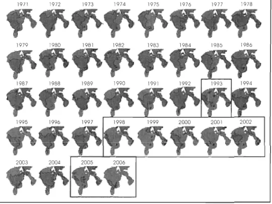
Figure 1. Couvertures historiques de glace de mer à la mi-juillet dans le SBH de 1971 à 2006 (M. Harvey; donées non publiées) ... 3
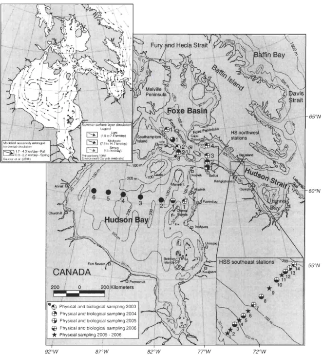
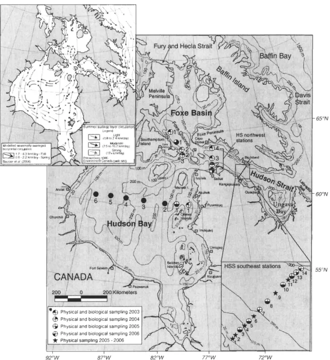
Figure 2. Localisations des stations d'échantillonnage dans le SBH pendant le programme MERICA-nord 2003-2006. En médaillon, le patron de circulation générale de la couche de surface pour les conditions estivales dans le bassin de Foxe, la baie d'Hudson et le détroit d'Hudson (adapté de Prinsenberg, 1986b; Saucier et al., 2004); Environnement Canada) . ... Station (FB3) visitée seulement en 2003 ... 10
2. LA TE SUMMER ZOOPLANKTON COMMUNITY STRUCTURE,
ABUNDANCE AND DISTRIBUTION IN THE HUDSON BA Y SYSTEM AND THEIR RELATIONS WITH ENVIRONMENT AL CONDITIONS, 2003-2006
Figure 1. Location of the sampling stations in the HBS during 2003-2006. The summer surface layer circulation is shown in the inset (adapted from Prinsenberg, 1986; Saucier et al., 2004; Environnement Canada). "'Station (FB3) sampled only in 2003 . ... 24
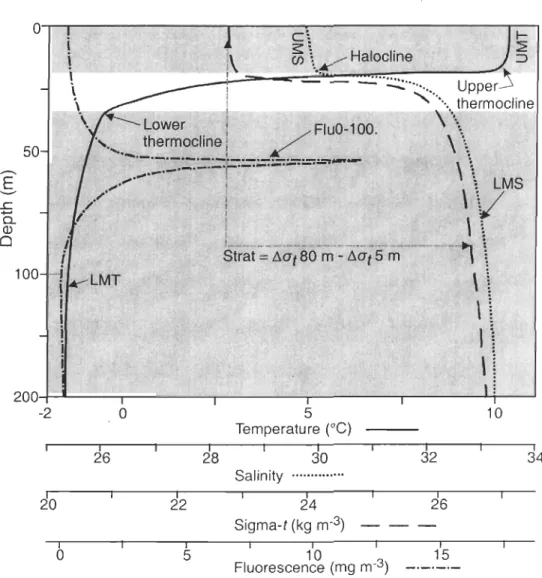
Figure 2. Sketch of typical vertical profiles of water temperature, salinity, sigma-t (crr) and chlorophyll fluorescence in the HBS. These data were used to calculate the upper mean tempe rature (UMT), lower mean tempe rature (LMT), upper mean sali nit y (UMS), lower mean sali nit y (LMS), stratification index (Strat) and integrated chlorophyll fluorescence from 0 to 100 m (FluO-100) ... 34
x
Figure 3. Water tempe rature distribution in Hudson Bay, Hudson Strait and Foxe Basin
from 2003 to 2006 ... 45
Figure 4. Salinity distribution in Hudson Bay, Hudson Strait and Foxe Basin from 2003 to
2006 ... 46 Figure 5. Chlorophyll fluorescence distribution in Hudson Bay, Hudson Strait and Foxe Basin from 2003 to 2006 ... 47
Figure 6. Variations of (A) chlorophyll a (chI a) concentration (via in vivo fluorescence),
(B) total zooplankton biomass and (C) total macrozooplankton abundance in the HBS
from 2003 to 2006. HB: Hudson Bay; HS: northwestern Hudson Strait; HSS:
southeastern Hudson Strait; FB: Foxe Basin. ChI a was integrated from surface to 100 m whereas zooplankton biomass and abundance were integrated from surface to bottom. In (B) and (C), mean and SD are shown for 2003 and 2004 ... 50 Figure 7. Variations of (A) total mesozooplankton abundance, (B) relative mero- and
holoplankton abundance and (c) relative copepod abundance in the HBS from 2003 to 2006. HB: Hudson Bay; HS: northwestern Hudson Strait; HSS: southeastem Hudson
Strait; FB: Foxe Basin. Zooplankton abundance was integrated from surface to
bottom. In (A), mean and SD are shown for 2003 and 2004. In (B) and (C), numbers above bars indicate total abundance (ind. mo2) ...•...•...•... 55
Figure 8. Two-dimensional non-metric multidimensional scaling (NMDS) ordination of the
zooplankton samples collected at 50 stations in the HBS during 2003-2006. The four groups of samples with similar taxonomic composition assessed with a cluster analysis
using the Bray-Curtis similarity are superposed to the NMDS. Each group of samples belongs to a distinct region of the HBS (global one-way ANOSIM test, R = 0.75, P :S
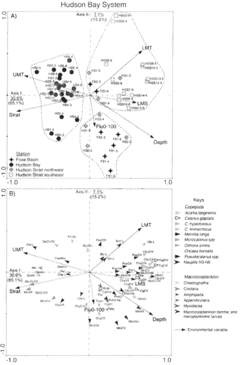
Figure 9. Redundancy analysis (RDA) ordination plots of axes 1 and II showing (A) sampling stations (symbols labelled: station-year) and (B) zooplankton taxonomie categories (coloured arrow tips) in relation to environmental variables (full black arrows) of data collected in the HBS during 2003-2006. Together axes 1 and II explain 37.7% of the total taxonomie variation (underlined values) and 80.3% of the taxonomie entry-environment relationship (values in parentheses). The model explains 47% of the total zooplankton variability within the HBS. For clarity, only taxonomie categories that fit 5% or more are shown in (B). Full names of environmental variables and of taxonomie categories are listed in Table 1 and in Tables 2 and 3, respectively . ... 62 Figure 10. Partial redundancy analysis (partial RDA) ordination plot of axes 1 and II showing sampling stations (symbols labelled: station-year) and zooplankton taxonomie categories (coloured arrow tips) in relation to environmental variables (full black arrows) of data collected in Hudson Bay during 2003-2006. Together axes 1 and II explain 31.6% of the taxonomie variability (underlined) and 60.0% of the taxonomie entry-environment relationship (values in parentheses). The model explains 46.4% of the total zooplankton variability within this area. For clarity, only taxonomie categories that fit 5% or more are shown. Similar group samples are encircled (dashed line) and the taxonomie categories that occurred more on eaeh group are shadowed.
Full names of environmental variables and of taxonomie categories are listed in Table 1 and in Tables 2 and 3, respectively ... 68 Figure 11. Redundancy analysis (RDA) ordination plot of axes 1 and II showing sampling stations (symbols labelled: station-year) and zooplankton taxonomie categories (coloured arrow tips) in relation to environmental variables (full black an'ows) of data collected in Foxe Basin and Hudson Strait during 2003-2006. Together axes 1 and II explain 35.6% of the taxonomie variability (underlined) and 72% of the taxonomie entry-environment relationship (values in parentheses). The model explains almost
Xll
50% of the total zooplankton variability within this area. For clarity, only taxonomic categories that fit 5% or more are shown. Similar group samples are encircled (dashed line) and the taxonomic categories that occurred more on each group are shadowed. Full names of environmental variables and of taxonomic categories are listed in Table 1 and in Tables 2 and 3, respectively ... 72 Figure 12. Variations of (A) total zooplankton biomass, and (B) Shannon' diversity index
(H') and Pielou's evenness index (l') and (C) species richness (S) of zooplankton in
the HBS from 2003 to 2006. HB: Hudson Bay; HS: Hudson Strait; HS: northwestem Hudson Strait; HSS: southeastem Hudson Strait; FB: Foxe Basin. Zooplankton biomass was integrated from surface to bottom ... 76 Figure 13. Relationships between (A) total zooplankton biomass and bottom depth, stratification index, upper mean salinity and upper mean temperature, (B) Shannon' diversity index (H') of zooplankton and stratification index, lower mean temperature and upper mean salinity and (C) species richness (S) and upper mean temperature, bottom depth and stratification index in the HBS during 2003-2006 ... 77
LISTE DES TABLEAUX
Table 1. Physical and biological characteristics of the sampling stations in the HBS from 2003 to 2006: bottom depth (Depth), upper mean temperature (UMT) , lower mean
temperature (LMT) , upper me an salinity (UMS), lower mean salinity (LMS),
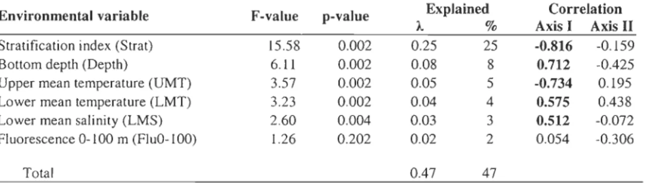
stratification index (Strat) and integrated chlorophyll fluorescence from 0 to 100 m (FluO-IOO) ... 29 Table 2. Occurrence and abundance of the macrozooplankton taxa present in the HBS during 2003-2006. Abbr.: abbreviation ... 39 Table 3. Occurrence and abundance of copepod taxa present in the HBS during 2003-2006. Abbr.: abbreviation ... 40 Table 4. Forward selection of environmental variables influencing the horizontal distribution of the zooplankton community in the HBS during 2003-2006 (Monte Carlo permutation test in RDA with 499 unrestricted permutations, p < 0.05). High correlations (i.e. r> 0.5) between environmental variables and the first 2 RDA axes are in boldo ... 61 Table 5. Summary of redundancy analysis (RDA) of 69 zooplankton taxonomic categories with six forward selected environmental variables (see Table 4) for the HBS during 2003-2006 ... 64 Table 6. Forward selection of environmental variables influencing the horizontal distribution of the zooplankton community in (A) the Hudson Bay (partial RDA) and the FB-HS) (RDA) during 2003-2006 (Monte Carlo permutation test in RDA with 499 unrestricted permutations, p < 0.05). High correlations (i.e. r> 0.5) between
XIV
Table 7. Summary of partial redundancy analysis (partial RDA) of 61 zooplankton taxonomie categories with six forward environmental variables (see Table 6) and sampling mon th as covariable for the Hudson Bay, and of RDA of 69 zooplankton taxonomie categories with six forward selected variables (see Table 6) for the Foxe Basin - Hudson Strait during 2003-2006 ... 73
LISTE DES ABRÉVIATIONS
Abréviations en français:
SBH
=
Système de la baie d'HudsonBH
=
Baie d'HudsonDH
=
Détroit d'HudsonBF
=
Bassin de FoxeMERICA = Mers intérieures du Canada
Abréviations en anglais:
CARC
=
Canadian Arctic Resources CommitteeHBS
=
Hudson Bay SystemHB
=
Hudson BayHS
=
Northwestem Hudson Strait (corresponding to 2003-2004 samplings)HSS = Southeastem Hudson Strait Section (corresponding to 2005-2006 samplings)
FB
=
Foxe BasinNMDS
=
Non-metric multidimensional scalingANOSIM = Analysis of si mi 1 arity
RDA
=
Redundancy analysispRDA
=
Partial redundancy analysisSD
=
Standard deviation CV=
Coefficient of variationDepth
=
Bottom depthUMT
=
Upper mean temperatureLMT
=
Lower mean temperatureUMS
=
Upper mean sali nit yLMS = Lower mean salinity
FluO-lOO = Integrated fluorescence form 0 to 100 m
Strat
=
Stratification index1
1. INTRODUCTION GÉNÉRALE
1.1. LE CHANGEMENT CLIMATIQUE DANS LE SYSTÈME DE LA BAIE D'HUDSON
Au cours du dernier siècle, le climat de la terre a connu un réchauffement d'environ
0,6
Oc
qui est non seulement relié à des événements naturels comme les variations durayonnement solaire ou de l'activité volcanique, mais plus potentiellement à l'augmentation
des concentrations de gaz à effets de serre d'origine anthropique (IPCC 200 1, 2007).
L'Arctique est l'une des régions où les changements climatiques provoquent actuellement
des bouleversements importants (Serreze et al., 2000). En effet, les données satellitaires de
1978 à 2003 montrent une diminution moyenne de la couverture de la glace de mer de 2
-3% par décennie, ce qui correspond à 350 000 km2 par année (Comiso et Parkinson, 2004).
Dans ce contexte, le système de la baie d'Hudson (SBH) n'est pas une exception puisqu'il
est considéré comme une région très sensible aux variations climatiques (Laidre et Haide
-Jorgensen, 2005). Dans la région de la baie d'Hudson (BH), la glace de mer s'y forme en
novembre et demeure typiquement jusqu'au mois de juin (Gough et Wolfe, 2000). Dans le
SBH, la répartition et l'étendue de la glace de mer étaient relativement constantes à la
mi-juillet entre 1971 et 1992 (Fig. 1). Toutefois, les conditions de la glace de mer ont été beaucoup plus variables et démontrent une tendance à la diminution depuis 1993. De plus, Markus et al. (2009) ont récemment démontré que la saison libre de glace dans SBH a été rallongée de plus de 20 jours entre 1992 et 2007, ce qui représente l'augmentation la plus
la multiplication anticipée par deux des concentrations atmosphériques de CO2 entraînera la
3 1971 1972 1973 1974 1975 1976 1977 1978
"
1979 1980 1981 1982 1984 1985"t'"
1987"
Figure 1. Couvertures historiques de glace de mer à la mi-juillet dans le SBH de 1971 à
Ces changements climatiques du milieu auront, sans aucun doute, des conséquences
sur la structure et le fonctionnement de l'écosystème marin du SBR (Stirling et al., 1999). Des recherches réalisées de 1981 à 2002 sur le Guillemot de Brünnich (Urïa lomvia) ont montré un changement dans l'alimentation des oisillons (Gaston et al., 2003). Durant la période étudiée, la principale source de nourriture pour les oisillons est passée de la morue
arctique (Boreogadus saïda) au capelan (Mallotus villosus) et au lançon (Ammodytes spp.).
Gaston et al. (2003) ont remarqué que le déclin de la morue arctique (une espèce qui est
fortement associée à la glace de mer pour son alimentation et pour fuir les prédateurs) et
l'augmentation dans l'abondance du capelan et du lançon (deux espèces qui sont plus
abondantes dans les eaux avec peu ou sans couvert de glace estival) étaient associés avec
un réchauffement général des eaux de la BR.
De plus, Gaston et Woo (2008) ont rapporté la présence récente de Petit pingouin
(Alea torda) dans la région de la BR. Cette espèce a été aperçue à l'île de Coats qui est
située à 300 km plus à l'ouest du site de nidification connu pour cette espèce. L'arrivée de
cet a1cidé coïncide avec l'augmentation de capelans et de lançons dans l'alimentation des
oisillons de Guillemots de Brünnich au même site d'étude. De plus, la disparition du Petit
pingouin est constatée lorsque le lançon (sa proie préférentielle dans le Canada atlantique)
disparaît également. Cette corrélation entre la présence de lançons et de Petit pingouins
suggère un lien entre l'arrivée de cet oiseau et l'augmentation de l'abondance de lançon
5
La morue arctique se nourrit principalement de copépodes et d'amphipodes planctoniques, d'amphipodes associés à la glace et de mysidacés. Cette espèce est le principal lien entre les niveaux trophiques inférieurs et les prédateurs supérieurs (e.g. les oiseaux et les mammifères marins) (Hop et al., 1997; S<ether et al., 1999). Le capelan et le lançon sont tous les deux des espèces planctonophages dont la diète est composée de copépodes (principalement de Calanus finmarchicus, mais aussi de C. hyperboreus) (Scott, 1973; Astthorsson et Gislason, 1997).
1.2. LE ZOOPLANCTON ET LES CHANGEMENTS CLIMATIQUES
Le SBH est considéré comme un "point chaud" pour la conservation marine par le Comité des Ressources Arctiques Canadiennes (CARC), en regard de l'importance de la biodiversité et l'influence de la dynamique de ses eaux sur tout l'ensemble du système (Beckmann, 1994). Ce système possède une grande richesse faunique, des microalgues à l'ours polaire. L'ours polaire dépend fortement de la glace de mer pour chasser et se nourrir de phoques au cours de la période hivernale et printanière. De plus, il symbolise ce système en étant au sommet du réseau alimentaire (Gough et Wolfe, 2001). Les microalgues qui croissent à la base de la glace de mer au printemps et dans la colonne d'eau (phytoplancton) (Homer, 1985) sont la principale source de nourriture pour la faune benthique et plusieurs espèces zooplanctoniques comme le copépode Calanus glacialis (Runge et Ingram, 1991). Le zooplancton est le principal phytophage dans la chaîne alimentaire océanique. Il joue un rôle primordial dans le transfert d'énergie entre les producteurs primaires et les
consommateurs des mveaux trophiques supérieurs. De plus, les orgamsmes zooplanctoniques jouent un rôle clé dans la pompe biologique, puisqu'ils transportent une part importante du carbone fixé par le phytoplancton au fond des océans par leur production de pélotes fécales (Richardson, 2008).
Le zooplancton est reconnu comme un bio-indicateur très sensible aux changements climatiques, car il répond rapidement aux variations de températures et des systèmes de courants océaniques en modifiant sa répartition spatiale (Hays et al., 2005).
Jusqu'à ce jour, la dynamique du zooplancton dans le SBH est encore peu connue. Peu de recherches portant sur l'abondance et la composition spécifique du zooplancton, en fonction des variables du milieu, ont été publiées. Le zooplancton a été étudié au sud
(Grainger et Sween, 1976), au sud-est (Hsiao et al., 1983), à l'est (Rochet et Grainger,
1987) et au nord-ouest et nord-est (Roff et al., 1980) de la BH. La première étude décrivant simultanément l'abondance et la composition du zooplancton dans différentes régions de la BH et du DH a été effectuée par Harvey et al. (2001). Cette étude a été réalisée en septembre 1993 et couvrait un large secteur situé entre la baie James au sud de la BH et la
baie d'Ungava dans le DH. Des études ont été également réalisées à l'est (Taggart et al.,
1989 ; Hudon et al., 1993), à l'ouest (Percy et al., 1992), et pour l'ensemble (Grainger, 1990) du détroit d'Hudson (DB) et dans le bassin de Foxe (BF) (Grainger, 1962).
7
1.3. OBJECTIFS DE L'ÉTUDE
La variabilité spatiale et interannuelle du zooplancton dans les trois régions hydrographiques du SBH n'a jamais été étudiée. Le programme nommé MERICA-nord (études des MERs Intérieures du CAnada) a été développé par le ministère des Pêches et Océans Canada de la Région Québec afin de suivre, comprendre et prédire les changements climatiques et ses effets sur la productivité et la biodiversité qui surviendront au cours des prochaines années dans le SBH (Saucier et al., 2003). Dans ce contexte, l'objectif principal
de ce travail est de décrire la structure de la communauté zooplanctonique, son abondance,
sa biomasse et sa répartition dans les trois régions du SBH et ses relations avec les conditions environnementales (i.e. l'indice de stratification, la température et la salinité des couches de surface, la température et la salinité des couches profondes, la fluorescence intégrée de 0 à 100 m et la profondeur du milieu) lors de quatre années d'échantillonnage
qui se sont déroulées à la fin des étés 2003 à 2006. Un deuxième objectif vise à identifier des tendances linéaires possibles entre la biomasse et indices de diversité du zooplancton et les gradients physiques qui pourraient être influencés par les changements climatiques.
1.4. LE SYSTÈME DE LA BAIE DE HUDSON
Le système de la baie d'Hudson (SBH) se situe dans les régions arctiques et subarctiques du Canada, entre 50 - 700N et 95 - 65°0 (Fig. 2). Il comprend: la baie
d'Hudson (BH), le détroit d'Hudson (DH) et le bassin de Foxe (BF) qui forment probablement, l'un des plus grands estuaires nordiques (Prinsenberg, 1984).
Cette région est connectée à l'est, aux eaux de l'océan Atlantique par la mer du Labrador (via le DH) et dans le nord avec les eaux arctiques provenant du détroit de Fury et Hecla (via le bassin de Foxe) (Prinsenberg, 1986b). Le SBH est principalement influencé par trois types d'eau: l'écoulement des rivières, l'eau de mer provenant de l'océan Arctique et l'eau de mer du courant de l'ile de Baffin (Straneo et Saucier, 2008). L'eau de la fonte de glace de mer serait la source la plus importante d'eau douce dans le cycle saisonnier de cette région, notamment dans le BF (Jones et Anderson, 1994). Le BF a une profondeur ne dépassant pas 100 m pour les régions à l'est et de 200 m pour la région située au sud dans le canal de Foxe (Prinsenberg, 1986c). La BH a une profondeur moyenne de 125 m caractérisée par une topographie du fond variable moins accidentée dans le sud et très accidentée dans le nord; ce qui lui donne une forme rectangulaire de 925 par 700 km, en ignorant les zones peu profondes du sud-est (Jones et Anderson, 1994; Prinsenberg, 1986b). Le BF et la BH sont tous deux connectés à la partie profonde du DH qui est un canal étroit (70-150 km) et long (-750 km) d'une profondeur moyenne entre 300 et 400 m (Drinkwater, 1986). Normalement, le nord du BF est recouvert de glace de la
mi-9
octobre au mois de septembre, tandis que la BR est entièrement couverte de glace lors de l'hiver et libre de glace au mois d'août et septembre (Prinsenberg, 1986c; Wang et al., 1994). Le DR est couvert de glace au -3/4 de l'année et commence normalement à être libre de glace à partir du début du mois d'août jusqu'à la fin octobre (Percy, 1990). Selon la répartition de la salinité estivale et les patrons de morcellement de la glace dans le BF, il y a une circulation cyclonique dans la région nordique du bassin avec un fort courant vers le sud (0.6 m S-I) le long de la péninsule de Melville. De plus, il y a dans la partie sud du
bassin un apport d'eau provenant du DR le long de la péninsule de Foxe et une sortie d'eau :
le long de l'île de Southampton (Prinsenberg, 1986c) (Fig. 2, coin supérieur droit). Les eaux de fond du BF ont une salinité plus élevée (causée par la libération de l'eau salée lors de la production et le vieillissement de la glace de mer) que les eaux provenant de l'océan Arctique par le détroit de Fury et Hecla et les eaux de fond provenant de l'est du DR. La couche supérieure d'eau saumâtre (salinité [S]
=
33.1) du BF a une épaisseur approximative de 25 m (Jones et Anderson, 1994). La température moyenne des eaux de surface est de -3 oC et est plus chaude dans la région du canal de Foxe (Prinsenberg,1
Fort Seve,"CANADA
_
/ 200 f
i o
'" ~ Physieal and biologie al sampling 2003
~ Physieal and biologieal sampling 2004
~ Physieal and biologieal sampling 2005
~ Physical and biological sampling 2006
*
Physical sampling 2005 -200692°W 87"W 65°N 600 N 55°N 82°W 77"W 72°W
Figure 2. Localisations des stations d'échantillonnage dans le SBH pendant le programme
MERICA-nord 2003-2006. En médaillon, le patron de circulation générale de la couche de
sutiace pour les conditions estivales dans le bassin de Foxe, la baie d'Hudson et le détroit d'Hudson (adapté de Prinsenberg, 1986b; Saucier et al., 2004); Environnement Canada).
11
Dans la BR, les données de bouteilles de dérive et la répartition spatiale de la salinité et de la température indiquent une circulation cyclonique dans la couche de surface (0.05 m S-I) .. La masse d'eau sortant le long de la côte est de la baie est relativement
chaude et de faible salinité (Prinsenberg, 1983; 1986a). Des simulations numériques récentes suggèrent qu'en absence de glace de mer, les eaux de la baie expérimenteraient de plus fortes activités de tourbillons en surface. Ces tourbillons seraient associés 1) aux forçages synoptiques du vent et à la présence d'un gyre cyclonique à grande échelle dans la partie ouest de la BR, et 2) aux plus forts courants à l'automne (0.02-0.05 m S-I) qui sont
deux fois plus élevées que ceux du printemps (Saucier et al., 2004) (Fig. 2, coin supérieur gauche). La circulation générale dans la baie causée par le vent et les courants de densité résultants de la dilution par les eaux de ruissellement des rivières. Ces eaux proviennent d'une grande aire de drainage (3.1 x 10⁶ km2) avec un débit annuel moyen de 2.1
x
104 m3 S-I (Prinsenberg, 1986b; 1988). Durant l'été, la BR est stratifiée verticalement avec uneforte pycnocline allant de 15 à 25 m; les températures des eaux de surface atteignent 12 oC et les eaux profondes -1.7 oC; la salinité de surface s'étend de 10 à 30 près des rivières majeur au centre et au nord-est de la BR, respectivement (Roff et Legendre, 1986). Les eaux profondes de la BR, lesquelles circulent elles aussi d'une façon cyclonique, sont le produit des eaux froides de surface de l'océan Arctique entrant 1) par le DR par l'ouest (via le détroit de Fury et de Recla, au nord du BF); 2) par le DR par l'est (qui coule vers j'ouest par le biais d'une extension du courant de Baffin); 3) et par les eaux plus chaudes et plus salées de l'Atlantique entrant en profondeur par le DR (Barber, 1967).
Dans le DH, la circulation de surface a trois principaux patrons: 1) un courant
.
entrant au SBH se dirigeant vers le nord-ouest le long de la rive sud de l'île de Baffin; 2) un courant sortant du SBH se déplaçant vers le sud-est le long de la rive nord du Québec, et qui éventuellement contribue au courant du Labrador; et 3) dans la moitié orientale du détroit, un écoulement à contre-courant vers le sud s'ajoutant au courant sortant du SBH (Drinkwater, 1986; LeBlond et al., 1981) (Fig. 2, coin supérieur gauche). Selon Straneo et Saucier (2008), les afflux d'eaux douces (S
=
33) du DB au SBB apportent -44 mSv (miIIi Sverdrup); ces écoulements d'eau hors du détroit de Davis sont donc des eaux arctiques qui circulent pour atteindre l'Atlantique Nord subpolaire. D'autre part, l'écoulement sortant du DH, apporte de l'eau douce et froide du SBH, le long de la côte du Québec, vers la mer du Labrador; ce flux s'étend de 40 à 50 km des côtes, avec des vitesses de 1 m S·l (Straneo etSaucier, 2008). Les sorties d'eaux du DH, transportent deux types de masses d'eau: des eaux plus douces (S
=
< 33) et très stratifiées sont acheminées entre juin et mars, et deseaux plus sa,Iées (> 33) et moins stratifiées sont acheminées sous les eaux douces, lors de la période de la sortie des eaux douces entre mars et juin. Il est estimé que 15% du volume et 50% de l'eau douce du courant du Labrador proviennent du DB (Straneo et Saucier, 2008). Cela influence grandement les propriétés et l'écosystème le long du plateau du Labrador (Straneo et Saucier, 2008). De façon globale, les marées de grandes amplitudes dans le DH (qui augmentent de 2 m à l'est de l'entrée à plus de 3,4 m près de Big Island, et qui décroissent à l'entrée ouest) et les forts courants tidaux (jusqu'à 2-3 m S·l) produisent un
mélange vertical intense, qui à une forte influence sur la stratification verticale de la colonne d'eau, de la température de l'eau et de la salinité ainsi que sur la productivité
l3
biologique locale dans différentes régions du détroit (Drinkwater, 1986; Drinkwater et
2. LA TE SUMMER ZOOPLANKTON COMMUNITY STRUCTURE, ABUNDANCE AND DISTRIBUTION IN THE HUDSON BA Y SYSTEM AND
15
ABSTRACT
Zooplankton communities were exarnined for the first time in three different hydrographic regions of the Hudson Bay system (HBS) in early August-early September
from 2003 to 2006. Sampling was conducted at fifty stations distributed along different
transects located in the Hudson Bay (HB), Hudson Strait (HS) and Foxe Basin (FB). The
variations in zooplankton biomass, abundance, taxonomic composition and diversity in
relation to environmental variables were studied using multivariate [non-metric
multidimensional scaling, one-way analysis of similarity (ANOSIM) and redundancy
analysis (RDA)] techniques. During aIl sampling years, the average total zooplankton
biomass (expressed in wet mass) was, on average, 4 times lower in HB (14.1 g m-2) than in
HS (64.2 g m-2) and FB (60.0 g m-2). Clustering samples by their relative species
compositions revealed no interannual variation in zooplankton community (ANOSIM test,
R
=
0.10, P > 0.05), but did reveal a markedly interregional variability between the threeregions (ANOSIM test, R
=
0.75, P:s
0.001). Water column stratification explained thegreatest proportion (25 %) of this spatial variability in the structure of zooplankton
communities within the HBS. According to the RDAs, the zooplankton taxa that contribute
most significantly to the separation of the three regions are: MicrocaLanus spp., Oithona
similis, Oncaea boreaLis, Aeginopsis Laurentii, Sagitta eLegans, Fritillaria sp., and larvae of
Cnidaria, Chaetognatha and Pteropoda in the HB; hyperiid amphipods in the FB; and
PseudocaLanus spp. CI-CV, CaLanus gLaciaLis CI-CVI, C. finmarchicus CI-CVI, C.
CVIf, Eukrohnia hamata, larvae of Echinodermata, Mollusca, Cirripedia, Appendicularia,
and Polychaeta in the northwestern and southeastern HS sections. In the HB, the
environmental variables analysed in a partial RDA allowed to distinguish three regions
inside the bay transects (HB West, Central, and East) with different environmental
gradients and zooplankton assemblages with Pseudocalanus spp. naupliar and CI-CVI, and
macrozooplankton benthic and meroplankton larvae showing higher occurrence in western lIB. In the HS, Calanoid species (mainly C. finmarchicus &
c.
glacialis) were mainly observed in the northern shore stations associated with the weakly stratified Arctic-NorthAtlantic waters coming from south western Davis Strait (inflow). In general, the RDA
models tested among the regions of the HBS were very consistent with its general surface layer circulation pattern for the summer condition in terms of environmental variables and distinct zooplankton assemblages. Overall, both the zooplankton biomass and diversity indices (H', ]' and S) were lower in the most stratified environment (i.e. lIB) thé:l.n in the deeper and more dynamic regions (i.e. FB & HS, respectively). The results of this work
show clearly that the structure in zooplankton communities is influenced by the
hydrodynamic conditions in the HBS that, trough their actions on temperature, salinity,
stratification, mixing conditions and depth strata, lead to the spatial differentiation of these
l7
INTRODUCTION
Estuarine systems in general are highly dynarnic and display distinctive physical
and chemical features that influence planktonic organisms in different ways (Sterza and
Fernandes, 2006). Salinity, more than any other variable, deterrnines the diversity in
estuaries (which decreases with distance from the sea) and distribution of zooplankton
within estuaries (Litle, 2000; Johnson and Allen, 2005). However, current systems could
play a major role in zooplankton distribution within a geographic area carrying species that
rnight be tolerant or not (Lance, 1963) to the changing conditions of the water masses they
are living in.
In these estuarine environments, it is common to find a sequence of zooplankton
assemblages along the salinity gradient with: i) euryhaline-freshwater species (at the
riverine end); ii) then estuarine species followed by euryhaline marine species (further
downstream); iii) stenohaline marine species (at the marine zone) (Litle, 2000). This
reflects the horizontal distribution of zooplankton species classically observed in estuarine
systems. In fact, brackish waters contain a mixture of typically brackish zooplankton plus
sorne particularly tolerant marine and fresh water species with more limited estuarine
distribution (Johnson and Allen, 2005).
In temperate ecosystems, the establishment of the seasonal therrnocline significantly
stratified conditions in summer-autumn (Ramfos et al., 2006). In estuaries, the stratification is an universal feature produced by the combined effects of temperature and salinity differences in the water column and its intensity depends strongly in the amount of freshwater input and on the intensity of wind and tidal mixing (Johnson and Allen, 2005).
The Hudson Bay system (HBS) is located in the Arctic and sub-Arctic regions of Canada. It is formed by: the Hudson Bay (HB), the Hudson Strait (HS) and the Foxe Basin (FB), which together make up one of the largest northern estuaries (Prinsenberg, 1984). Bliefly, RB is one of the biggest inland seas in the Northern Hemisphere (830 x 103 km2) (Prinsenberg, 1984). This region is characterised by a great fresh water input coming from the surrounding rivers and also by the seasonal sea-ice melting, which give it estuary-like charactelistics: a two water layer circulation pattern separated by a strong pycnocline located between 5 and 25 m (Roff and Legendre, 1986). The massive intrusions of continental waters drive a horizontal cyclonic circulation pattern on the surface layer of the RB, which is characterized by fresher and less dense waters than those entering between Southampton and Coats Islands. The fresh surface waters mix with the numerous local river plumes and slowly circle the bay before exiting by the southern shore of the HS towards the Labrador Sea (Pett and Roff, 1982).
Earlier studies showed that the horizontal distribution of the macro- and mesozooplankton in the RBS can be influenced by the local environmental gradients and water mass circulation. For example, Grainger (1962) distinguished two groups of
19
zooplankton in the FB. The first one with species showing the influence of arctic waters entering the basin from the north (i.e. the copepods C. glacialis, C. hyperboreus, and the
amphipod Themisto libellula, amongst others), and the second constituted of subarctic
species introduced from the south (i.e. C. finmarchicus, Themisto abyssorum). Rochet and
Grainger (1987) identified different zooplankton assemblages in eastem RB waters accordingly to the salinity gradients and water masses present there. In their study, the
zooplankton component (e.g. the cnidarians Aglantha digitale and Aeginopsis laurentii) in
the eastem part of the bay showed clearly the influence of arctic waters aIl over the area,
whereas zooplankton indicative of estuarine conditions (e.g. the copepods Centropages
abdominalis and Eurytemora herdmani) were confined to the southeastem RB area where low salinities prevaii.
More recently Harvey et al. (2001) identified four different zooplankton assemblages within the environmental gradients recorded, sali nit y in particular, over a large
sector close to the shores extending from the entrance of James Bay, south of HB, to the
southeastem HS shore. In their study, the euryhaline copepods Acartia longiremis and
Centropages hamatus represented the first group in the less saline waters of southeastem
RB, while the higher zooplankton biomasses, featured by Calanus finmarchicus and C.
glacialis, characterized a more saline surface water portion at the end of the HS transect.
During the last century, the oceanic and terres tri al planet surfaces have warmed (about 0.6 OC) mainly due to the increase of the greenhouse effect gases coming from
human origin activities (IPCC, 2001, 2007). The Arctic is one of the regions where climate
changes are currently causing serious damages (Serreze et al., 2000). In this context, the
HES is no exception since, it is considered as a very sensitive region to climate variations
(Laidre and Heide-Jprgensen, 2005).
According to the Canadian first-generation coupled general circulation model
(CGCM 1), the doubling of the CO2 atmospheric concentrations will involve the quasi total
disappearance of sea-ice in the HE (Gough and Wolfe, 2001), which could have important
consequences over the local biota and the entire ecosystem (Stirling et al., 1999). The
temporal change in the sea-ice cover in the HES during mid-July from 1971 to 2006 is
shown in Fig. 1 of the general introduction (chapter 1.1). Between 1971 and 1992, the
spreading and extension of the sea-ice cover were relatively constant. But since 1993,
sea-ice conditions have been more variable and instable (Fig. 1) showing a trend toward earlier
melt onset in spring and also later freeze-up in fall (Markus et al., 2009). Overall, the melt
season in HE has lengthered by almost 20 da ys from 1992 to 2007 (Markus et al., 2009).
These changes in sea-ice dynamics suggest that the HBS are already responding to climate
walming with potential consequences on the water properties and circulation, the
freshwater transport towards the Labrador Sea, and the biological productivity of this
arctic/subarctic system (Saucier et al., 2004).
Apart from playing a fundamental role in marine food webs, zooplankton has been
21
as weIl as oceanic CUITent variations by modifying its spatial distribution (Hays et al., 2005; Richardson, 2008). Information on zooplankton dynamics in the HBS is scarce. Only a few papers on specific zooplankton groups in relation to the local physical variables, limited to sorne regions of the HB, FB and HS specifically, have been published (Grainger, 1962, 1990; Grainger and McSween, 1976; Roff et al., 1980; Hsiao et al., 1984; Rochet and Grainger, 1988; Taggart et al., 1989; Percy et al., 1992; Hudon et al., 1993; Harvey et al., 2001). The spatial and interannual zooplankton variation for three different hydrographic regions of the HBS has never been studied. The MERICA (MERs Intérieures du CAnada) program has been developed by the DFO Quebec Region to follow, understand, and predict the future climate changes and their effects on the productivity and biodiversity of the HBS (Saucier et al., 2003).
In this context, the mam objective of this work is to describe the zooplankton community structure, abundance, biomass and distribution in the HBS and its relationship with the environmental conditions during late summers of 2003 to 2006. A second objective is to identify possible linear trends between zooplankton distribution and physical gradients that may be influenced by climate changes. This will allow us to propose different scenarios on the potential effects of climate changes on the zooplankton communities in
sub-arctic regions. Our working hypothesis is that the structure of the zooplankton communities is influenced by the water depth and local hydrodynamic conditions which through their actions on the water masses propelties (i .e. temperature, salinity and
stratification intensity) will lead to spatial differentiation in zooplankton communities in the
HBS (from 2003 to 2006).
MA TERIALS AND METHODS
Studyarea
Situated between 50 - 700N and 95 - 65°W (Fig. 1), the HBS is a large
subarctic/arctic estuarine basin with a seasonally complete cryogenie cycle (Straneo and Saucier, 2008). Eastward, this region is connected to waters of the Atlantic Ocean by the
Labrador Sea (through HS), and in the north to the waters of the Canadian Arctic by Fury
and Hecla Strait (through PB) (Fig. 1) (Prinsenberg, 1986b). The HBS is mainly influenced
by three water types: river runoff, seawater from the Arctic Ocean and seawater from the
Baffin Island CUITent. Sea-ice melt water is the most significant source of freshwater in the
seasonal cycle of the area, notably FB (Straneo and Saucier, 2008). Together, HB and FB
covers an area of about 106 km2. FB is no more than 100 m deep with the shallowest regions in the east, and the deepest (200 m) in the south at Foxe Channel; the latter, along
with southwestem FB, are considered to be an extension of HS (Prinsenberg, 1986c). RB
has a mean depth of 125 m with variable bottom topography, more gentle in the south and
deeper trenches in the north; it has a rectangular shape of 925 by 700 km, ignoring the
southeastem shallow area (Jones and Anderson, 1994; Prinsenberg, 1986b). Both FB and
HB are connected to the deeper HS, which is a naITOW (70-150 km) and long (-750 km)
23
conditions are found in September and freeze-up begins by mid-October in northem FB, whereas RB is ice covered in winter and ice-free in August and September (Prinsenberg, 1986c; Wang et al., 1994). RS is ice-covered -3/4 of the year, and normally being ice free from early August untillate October (Percy, 1990).
{
-, i
200 ! 0
i .
.. ~ Physical and biological sampling 2003
~ Physical and biological sampling 2004
~ Physical and biological sampling 2005
~ Physical and biological sampling 2006
*
Physical sampling 2005 . 2006 92°W 65°N 600N 55°N 82°W 77°W 72°WFigure L Location of the sampling stations in the HBS dUling 2003-2006. The summer
surface layer circulation is shown in the inset (adapted from Plinsenberg, 1986; Saucier et al., 2004; Environnement Canada). ""Station (FB3) sampled only in 2003.
25
According to the summer salinity distribution and ice breakup patterns in FB, there is a cyclonic circulation in northern region of the basin with a strong southerly CUITent (0.6 m S·l) along the Melville Peninsula (which is a southward continuation of the Arctic water through Fury and Hecla Strait) (Prinsenberg, 1986c). Additionally, in the southern part of the FE there is an inflow of waters from HS along Foxe Peninsula, and an outflow along Southampton Island (Prinsenberg, 1986c) (Fig. 1, upper left corner). Particularly, FB has higher salinity bottom water (because of the brine released during sea-ice production and aging of) than waters entering from the Arctic Ocean and those from the bottom water at eastern HS; the freshwater layer (S
=
33.1) is around 2.5 m (Jones and Anderson, 1994). Summer surface water temperatures are -3 oC, being warmer in the Foxe Channel area (Prinsenberg, 1986c).In HE, bottle drift data and sali nit y and temperature distributions indicate a cyclonic surface layer circulation (0.05 m S-l) without north westward inflow, and an eastward surface outflow that moves along the eastern shore, leaving the bayas a warm and fresher water mass (Prinsenberg, 1983; Prinsenberg, 1986a). Furthermore, recent data models show that during the ice-free periods the waters of the bay experiment stronger surface eddy activity associated with the synoptic wind forcing and the presence of a large sc ale cyclonic gyre in the western half of the HE, with strongest CUITents in the fall (0.02-0.05 m S-l) and half lower in spring (Saucier et al., 2004). The mean circulation in the bay is a combination of wind and density-driven CUITents resulting from dilution by river runoff; the latter cornes from a large drainage area (3.1 x 10⁶ km2) with a yearly mean discharge of 2.1 x 10⁴m3 . S-l
(equals to an annual addition of a 0.78m layer of freshwater if spread out over the entire surface of the bay) (Fig. 1, upper left corner) (Prinsenberg, 1986b; 1988). Remarkably, during the summer RB is vertically stratified with a strong pycnocline ranging 15-25 m; surface salinity ranges 10 to 30 from near major river systems to central and northeastem RB, respectively; summer surface water temperatures reach 12 oC, and the deep waters -1.7 oC, close to the freezing point. The resident time of deep RB waters lies between 4-14 years, increasing towards the centre of the bay (Pett and Roff, 1982; Roff and Legendre,
1986). RB deep waters, which are also considered to circulate cyclonically, are the product
of: cold surface Arctic Ocean waters entering HS from the west (via Fury and Hecla Strait -FB); from the east (via a westward flowing extension of the Baffin cUITent); and warmer,
more saline Atlantic waters entering HS at depth (Barber, 1967).
In HS, the surface circulation has three mam patterns: 1) a CUITent flowing
northwestward along southern Baffin Island (inflow); 2) a southeastward CUITent flowing along the Quebec shore (outflow), which join that from Davis Strait and West Greenland
recirculation CUITent to form Labrador CUITent; and 3) a southward cross-channel flow in
the eastem half of the strait (Drinkwater, 1986; LeBlond et al., 1981) (Fig. 1, upper Ieft corner). According to Straneo and Saucier (2008), the HS inflow supplies -44 mSv (milli Sverdrup) of freshwater (S
=
33) to the HBS; this water flows out of Davis Strait and thusis of Arctic influence. These waters are weakly stratified due to high vertical mixing at the
eastern entrance of the HS. On the other hand, the HS outflow carries fresh, cold waters from the HBS, along the coast of Québec, towards the Labrador Sea; this flow ex tends
45-27
50 km off the coast, with velocities (1 m S-l) dominated by strong tides (mostly
semidiurnal) exceeding 8 m. The outflow carries two classes of water masses: fresher (S
=
< 33) and highly stratified waters exported between June and March, and more saline (>
33) and less stratified waters exported beneath the freshwaters, during the fresh outflow
period between March and June (Straneo and Saucier, 2008). It is estimated that 15 % of
the volume and 50 % of the fresh water carried by the Labrador Current is due to the HS
outflow, reflecting a large impact on the properties and ecosystem along the Labrador Shelf (Straneo and Saucier, 2008). Overall, high tidal elevations in HS (increasing from 2 m at the eastern entrance to over 3.4 m near Big Island, and th en decreasing at the western
entrance), and strong tidal currents (up to 2-3 m S-l) that produce intense vertical mixing,
through bottom-generated turbulence, have strong local influence on the vertical
stratification of the water column, temperature and salinity properties, and local biological
production in different areas of the strait (Drinkwater, 1986; Drinkwater and Jones, 1987).
Sampling program
Sampling was carried out in the Hudson Bay system from 1 to 14 August in 2003
and 2004 and from 31 August to 10 September in 2005 and 2006, on board of the CCGS
Des Groseilliers in 2003 and Pierre Radisson during 2004-2006 (Fig. 1). A total of 56
stations were visited over the four years. Physical and biological data were collected at 5-6
stations along a longitudinal transect in the RB from 2003 to 2006, at 4 stations along a
cross-channel transect in the southeastem HSS in 2005 and 2006 (see Fig. 1 and Table 1). The position of the HSS transect during 2005-2006 corresponds to the transect conducted by Drinkwater (1986). The FB was sampled at 3 stations in 2003, at 2 stations in 2004 and at 1 station in 2005 and 2006. The position of the station PB 1 in Foxe Channel was relocated ca. 50 km southeast during 2004-2006 because of the presence of a thick sea ice cover north of the channel during surnrner 2004.
At each station, vertical profiles of water temperature, salinity, density (sigma-t, crI) and in vivo fluorescence down to about 10 m above the bottom were measured with a Sea-Bird Electronics SBE 91l+CTD and a Wetstar mini fluorometer (model 9512008) attached to a rosette sampler. Subsamples for chlorophyll a (chI a) determination were collected at 48 stations (from 56 visited over the four years) at 0, 5, 15, 25, 50, 75, 100, and 250 m (when depth permitting) with 10-1 Niskin bottles mounted on the rosette system.
29
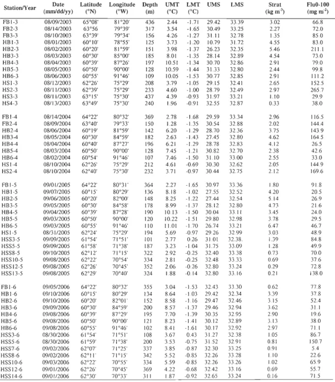
Table 1. Physical and biological characteristics of the sampling stations in the HBS from 2003 to 2006: bottom depth (Depth), upper me an tempe rature (UMT), lower mean temperature (LMT), upper mean salinity (UMS), lower mean salinity (LMS), stratification index (Strat) and integrated chlorophyII fluorescence from 0 to 100 m (FluO-lOO).
StationlYear (mmlddlyy) Date Latitude Longitude Depth UMT LMT UMS (oN) (OW) LMS SIrat FluO-lOO
(m) (OC) COC) (kg m') (mg m") FBI-3 08/0912003 65°08' 81 °20' 436 2.44 -1.71 29.42 33.39 3.02 66.8 FB2-3 08/14/2003 63°56 79°39' 317 3.54 -1.65 30.49 33.25 2.27 72.0 FB3-3 08/1012003 63°39' 79°34' 156 4.26 -1.27 31.11 32.78 1.35 85.0 HBI-3 08/0112003 60°10' 78°55' 125 3.73 -1.20 10.79 31.72 4.55 83.0 HB2-3 08/0212003 60°20' 81°59' 151 3.98 -1.37 26.23 32.35 5.46 211.1 HB3-3 08/0312003 60°30' 85°00' 185 8.01 -1.35 28.14 32.89 4.54 73.0 HB4-3 08/0412003 60°39' 87°26' 197 10.51 -1.34 30.70 32.86 2.91 79.0 HB5-3 08/05/2003 60°50' 90°00' 128 10.59 -1.44 31.33 32.80 2.44 99.8 HB6-3 08/0612003 60°55' 91°46' 109 10.05 -1.53 30.77 32.85 2.91 111.2 HSI-3 0811212003 62°26' 75°29' 208 3.79 -1.05 29.15 32.41 2.65 152.5 HS2-3 08/1112003 62°39' 75°29' 233 4.60 -1.00 28.79 32.49 2.97 265.7 HS3-3 08/11/2003 63°15' 75°30' 437 4.39 -0.93 31.97 33.21 1.10 29.9 HS4-3 08/13/2003 63°49' 75°30' 240 1.96 -0.91 32.55 32.87 0.33 38.0 FBI-4 08/14/2004 64°22' 80°32' 369 2.78 -1.68 29.59 33.34 2.96 116.5 FB2-4 08/0912004 63°40' 79°33' ISO 1.28 -135 30.54 32.88 2.02 144.4 HB2-4 08/0612004 60°19' 81°59' 142 6.20 -1.29 28.70 32.36 3.75 143.9 HB3-4 08/05/2004 60°30' 84°59' 182 2.63 -1.43 27.45 32.80 4.62 164.5 HB4-4 08/0412004 60°40' 8r21' 196 6.21 -1.29 28.78 32.83 4.12 26.5 HB5-4 08/0312004 60°50' 90°00' 128 7.45 -1.21 30.82 32.70 2.38 42.6 HB6-4 08/0212004 60°54' 91°46' 107 7.46 -1.50 31.10 33.00 2.55 33.0 HSI-4 08/10/2004 62°26' 75°29' 212 4.61 -0.69 30.30 32.62 2.05 144.9 HS2-4 08/10/2004 62°40' 75°30' 232 3.71 -0.97 30.44 32.75 2.12 169.6 FBI-5 09/01/2005 64°22' 80°31' 364 2.27 -1.65 30.97 33.36 1.80 91.8 HBI-5 09/07/2005 60°15' 80°29' 136 8.18 -1.02 27.55 32.52 4.20 20.5 HB2-5 09/06/2005 60°20' 82°00' 148 8.25 -1.22 27.44 32.54 5.14 26.9 HB3-5 09/0512005 60°30' 84°58' 178 8.99 -137 28.12 32.80 4.73 21.6 HB4-5 09/04/2005 60°39' 87°28' 190 10.13 -1.50 30.04 33.11 3.45 24.0 HB5-5 09/03/2005 60°50' 90°00' 120 10.22 -1.51 29.80 32.98 3.78 29.5 HB6-5 09/03/2005 60°55' 91°46' 110 11.01 -1.70 26.74 33.21 6.47 46.7 HSI-5 08/3112005 62°24' 75°29' 194 5.69 -0.97 29.26 32.99 3.03 48.9 HSS3-5 09/09/2005 61 °54' 71°51' 101 2.77 0.26 31.01 32.38. 1.39 84.8 HSS5-5 09/09/2005 61 °58' 71 °38' 187 3.23 -1.04 31.75 33.09 1.28 49.9 HSS8-5 09/10/2005 62°12' 71°15' 322 2.92 -0.25 32.40 33.38 0.73 70.0 HSSIO-5 09/08/2005 62°22' 70°54' 334 2.81 -0.25 32.48 33.33 0.69 37.6 HSSI2-5 09/08/2005 62°26' 70°45' 352 2.06 -0.26 32.80 33.24 0.29 72.8 HSSI3-5 09/08/2005 62°29' 70°40' 324 1.88 -0.14 32.80 33.16 0.21 138.0 FBI-6 09/0512006 64°22' 80°32' 355 3.04 -1.53 32.43 33.30 0.62 77.8 HBI-6 09/10/2006 60°15' 80°29' 134 8.64 -1.03 29.42 32.34 3.39 37.8 HB2-6 09/10/2006 60°20' 82°01' 152 8.58 -1.16 29.47 32.46 3.15 52.4 HB3-6 09/0912006 60°30' 84°59' 200 8.57 -137 29.46 32.94 3.62 31.1 HB4-6 09/0812006 60°39' 8r 29' 195 770 -1.39 30.35 32.95 2.90 19.6 HB5-6 09/08/2006 60°50' 90°00' 121 8.23 -1.41 30.12 32.89 3.13 38.0 HB6-6 09/08/2006 60°55' 91 °46' 102 8.41 -1.61 30.17 32.92 2.97 71.1 HSS3-6 08/3012006 61 °54' 71°51' 108 3.67 0.43 31.27 32.38 1.05 86.7 HSS5-6 08/30/2006 61°59' 71°38' 200 3.53 -0.75 31.52 32.91 0.81 150.7 HSS7-6 09/0212006 62°01' 71 °25' 337 3.85 -0.87 32.30 33.25 0.91 5.4 HSS8-6 09/0212006 62°11 ' 71 °15' 342 5.52 -0.85 32.26 33.28 1.10 22.6 HSSIO-6 09/03/2006 62°22' 70°55' 334 5.59 -0.85 32.26 33.26 1.02 65.9 HSSI2-6 09/01/2006 62°26' 70°45' 369 4.22 -0.68 3242 33.16 0.69 55.7 HSSI4-6 09/01/2006 62°30' 70°33' 311 1.87 -0.92 32.65 33.24 0.16 71.5
Two 500-ml subsamples were filtered through 25 mm Whatman GF/F fiber glass
filters (nominal pore size of 0.7 jlm). Concentrations of chI a were measured on board the
ship with a Turner Designs TD-700 fluorometer, after 18 h of pigment extraction in 90%
acetone at 4°C in the dark (Parsons et al., 1984). The extracted chI a concentration was
used to calibrate the output of the Rosette fluorometer at each station, using Model l linear
regression (Sokal and Rohlf, 1995).
Immediately following the rosette cast, zooplankton samples were collected at a
total of 50 stations from ca. 10 m above the bottom to the surface with vertical tows at
speed of 1 m S-I, using a 0.75 m diameter ring net, equipped with a 202 jlm-mesh net. At
each station, the amount of filtered seawater (m-3) by the net was estimated using a General
Oceanics electronic flowmeter (model 2031H). Three vertical tows per station were carried
out in 2003 and 2004 and only one in 2005 and 2006. Ali sampling was performed during
daylight hours.
The zooplankton samples were preserved in 4% buffered formaldehyde, and
analyzed in two steps in Iaboratory: 1) larger organisms, defined here as macrozooplankton
(length >2 mm, e.g. euphausiids, amphipods, chaetognaths, cnidarians, pteropods), were
sorted, identified to species level (when possible), counted, and weighed individually by
taxa (wet mass: WM), using a Mettler PC4400 precision balance (± 0.01 g); 2) after
macrozooplankton removal, samples were split in two half (using a Folsom splitter) to
31
zooplankton orgamsms (length <2 mm, e.g. copepods and macrozooplankton larvae) defined here as mesozooplankton (second half).
The first haif of the samples containing mesozooplankton (including
macrozooplankton larvae) was filtered through pre-weighed Whatman GF/A filters with a
vacuum pump during 10 seconds and then weighed with a Mettler PC4400 precision
balance (± 0.01 g) to obtain by difference the WM. Since sorne samples contained
phytoplankton cells, especially those collected in the HE, the contribution of phytoplankton
to total plankton biomass was estimated for these samples. To do this, a 10 ml aliquot of the
second half sample was taken with a Stempel pipette and sorted into two fractions (i.e.
zooplankton organisms and phytoplankton cells) under a binocular dissecting microscope.
Both fractions were then filtered through pre-weighed Whatman GF/A filters and weighed
with a Mettler PC4400 precision balance (± 0.001 mg). The contribution of phytoplankton
to the total plankton (i.e. phytoplankton + zooplankton) wet mass ranged from 0 to 78%
(mean ± SD
=
34.9 ± 21.7%) in the HB during 2003-2006. Similar results were obtainedfrom zooplankton and phytoplankton dry masses measured on selected samples. Hence, our
wet mass mesozooplankton data were corrected for the presence of phytoplankton cells.
The second half of the samples for mesozooplankton identification and enumeration
was diluted in aliquots taken with a Folsom splitter or a Stempel pipette, depending on the
to 1/200 of the total sampJe. Then, the diluted subsample containing zooplankton was placed into a slide counting chamber and examined under a binocular dissecting microscope. Copepods were identified taken into account their life stages (i.e. naupliar (N), copepodite (C), adult male (m) and aduJt female (f)). For Calanus finmarchicus, Euchaeta norvegica, Metridia longa and Pseudocalanus spp. onJy naupliar stages from N3-N6 were counted due to the mesh size (>202 Jlm) of the net used during this study which exc1udes
the smaIJer individuals. A minimum of 400 individuals was counted in each counting chamber. The following references were used for zooplankton identification: Rose (1970),
Shi (1977), Smith (1977), amongst others. In total, 32 and 54 taxonomie categories were identified for the macrozooplankton and planktonic copepods, respectively. In the present study, biomass and abundance of zooplankton were expressed in g WM m·2 and in ind. m-2,
respecti vel y.
Data analysis
The physical and biological variables collected at the 50 net tow stations over the 4 sampling years aIJowed us to establish 3 data matrices composed of: 1) environmental variables (inc1uding chI a and fluorescence), 2) zooplankton abundances, and 3)
zooplankton biomasses. Figure 2 illustrates the environmental variables computed from the
vertical profiles obtained by the Rosette CTD-fluorometer. At each station, the depth of maximum and minimum vertical gradients in water temperature (L1 TI L1Z) was used to deterrnine the depth of the upper and lower limits of the thermocline, respectively. In
33
addition, the depth of the maximum vertical gradient in salinity (t::.S/6,Z) was used to determine the halocline depth. Within these zones, we calculated: 1) the upper (UMT) and Iower (LMT) mean temperature above the upper and Iower thermocline limit, respectively,
2) the upper mean sali nit y (UMS) above the halocline, 3) the Iower mean salinity (LMS) below the Iower thermocline limit, and 4) the integrated chI a fluorescence from 0-100 m
(FluO-lOO) (Fig. 2). The stratification index (Strat) was computed from the difference in crt
between 80 m and 5 m (!::.crt ). Rence, the environmental data matrix was composed of 7 variables (i.e. UMT, UMS, LMT, LMS, Strat, FluO-lOO and bottom depth). Contour plots
of water temperature, salinity and chI a fluorescence were produced with the Ocean Data
O.-.---.~~--~---~---.-~ c~ r ..c
....
Q. (])o
50 100!
\
.
~
\.
~
Halocline3
: -" - - ...:: .. ~... upper~l
"
...
.
..
thermocline Lower Il FluO-100. \ \" ·, ..._.~hermOCline
!
/ \ \ .-._._._.-r-._._._._._.:y... ....
· .... ·_·-·-·_·-
f
·_·_·_·_·_·-
,
\
\
LMS / 1\\.~
/
.
,/ 1 ~'
!
\
\
Strat
-:;~
at80
-
m
-
:
~at5
-
m
~---"~
·
\
\
\
\
~
1l
\ l
2004-~----r---~---~---~~---~--~ -2 ~O io
i 26o
1 22 i 5 1 28 5 10 Temperature (oC) 1 1 i 30 32 34 Salinity ... 1 1 24 26 Sigma-t (kg m-3) ----i i 1 i 10 15 Fluorescence (mg m-3) _._._.-Figure 2. Sketch of typical vertical profiles of water temperature, salinity, sigma-t (ac) and
chlorophyll fluorescence in the HBS. These data were used to calculate the upper me an
temperature (UMT), lower mean temperature (LMT), upper me an salinity (UMS), lower
mean sali nit y (LMS), stratification index (Strat) and integrated chlorophyll fluorescence