Dealing with heterogeneity in the prediction of clinical diagnosis

Université de Montréal

Dealing with heterogeneity in the prediction of clinical diagnosis

par

Christian Langlois Dansereau

Département d’informatique et de recherche opérationnelle Faculté des arts et des sciences

Thèse présentée à la Faculté des études supérieures en vue de l’obtention du grade de Philosophiæ Doctor (Ph.D.)

en informatique

Août, 2017

RÉSUMÉ

Le diagnostic assisté par ordinateur est un domaine de recherche en émergence et se situe à l’intersection de l’imagerie médicale et de l’apprentissage machine. Les données médi-cales sont de nature très hétérogène et nécessitent une attention particulière lorsque l’on veut entraîner des modèles de prédiction. Dans cette thèse, j’ai exploré deux sources d’hétérogénéité, soit l’agrégation multisites et l’hétérogénéité des étiquettes cliniques dans le contexte de l’imagerie par résonance magnétique (IRM) pour le diagnostic de la maladie d’Alzheimer (MA). La première partie de ce travail consiste en une introduction générale sur la MA, l’IRM et les défis de l’apprentissage machine en imagerie médicale. Dans la deuxième partie de ce travail, je présente les trois articles composant la thèse. Enfin, la troisième partie porte sur une discussion des contributions et perspectives fu-tures de ce travail de recherche. Le premier article de cette thèse montre que l’agrégation des données sur plusieurs sites d’acquisition entraîne une certaine perte, comparative-ment à l’analyse sur un seul site, qui tend à diminuer plus la taille de l’échantillon aug-mente. Le deuxième article de cette thèse examine la généralisabilité des modèles de prédiction à l’aide de divers schémas de validation croisée. Les résultats montrent que la formation et les essais sur le même ensemble de sites surestiment la précision du modèle, comparativement aux essais sur des nouveaux sites. J’ai également montré que l’entraînement sur un grand nombre de sites améliore la précision sur des nouveaux sites. Le troisième et dernier article porte sur l’hétérogénéité des étiquettes cliniques et pro-pose un nouveau cadre dans lequel il est possible d’identifier un sous-groupe d’individus qui partagent une signature homogène hautement prédictive de la démence liée à la MA. Cette signature se retrouve également chez les patients présentant des symptômes mod-érés. Les résultats montrent que 90% des sujets portant la signature ont progressé vers la démence en trois ans. Les travaux de cette thèse apportent ainsi de nouvelles con-tributions à la manière dont nous approchons l’hétérogénéité en diagnostic médical et proposent des pistes de solution pour tirer profit de cette hétérogénéité.

Mots clés: Hétérogénéité, Maladie d’Alzeimer, Apprentissage machine, Multi-site, Biomarqueur.

ABSTRACT

Computer assisted diagnosis has emerged as a popular area of research at the intersection of medical imaging and machine learning. Medical data are very heterogeneous in nature and therefore require careful attention when one wants to train prediction models. In this thesis, I explored two sources of heterogeneity, multisite aggregation and clinical label heterogeneity, in an application of magnetic resonance imaging to the diagnosis of Alzheimer’s disease. In the process, I learned about the feasibility of multisite data aggregation and how to leverage that heterogeneity in order to improve generalizability of prediction models. Part one of the document is a general context introduction to Alzheimer’s disease, magnetic resonance imaging, and machine learning challenges in medical imaging. In part two, I present my research through three articles (two published and one in preparation). Finally, part three provides a discussion of my contributions and hints to possible future developments. The first article shows that data aggregation across multiple acquisition sites incurs some loss, compared to single site analysis, that tends to diminish as the sample size increase. These results were obtained through semi-synthetic Monte-Carlo simulations based on real data. The second article investigates the generalizability of prediction models with various cross-validation schemes. I showed that training and testing on the same batch of sites over-estimates the accuracy of the model, compared to testing on unseen sites. However, I also showed that training on a large number of sites improves the accuracy on unseen sites. The third article, on clinical label heterogeneity, proposes a new framework where we can identify a subgroup of individuals that share a homogeneous signature highly predictive of AD dementia. That signature could also be found in patients with mild symptoms, 90% of whom progressed to dementia within three years. The thesis thus makes new contributions to dealing with heterogeneity in medical diagnostic applications and proposes ways to leverage that heterogeneity to our benefit.

CONTENTS

RÉSUMÉ . . . ii

ABSTRACT . . . iii

CONTENTS . . . iv

LIST OF TABLES . . . viii

LIST OF FIGURES . . . ix

LIST OF APPENDICES . . . xii

LIST OF ABBREVIATIONS . . . xiii

DEDICATION . . . xiv

ACKNOWLEDGMENTS . . . xv

CHAPTER 1: INTRODUCTION . . . 1

1.1 General context . . . 1

1.2 Alzheimer’s disease . . . 2

1.3 Overview of magnetic resonance imaging . . . 5

1.3.1 Overview of structural magnetic resonance imaging . . . 5

1.3.2 Overview of functional magnetic resonance imaging . . . 7

1.4 Preprocessing . . . 9

1.5 Resting-state connectivity . . . 11

1.6 Multisite . . . 15

1.7 Prediction of clinical diagnosis using medical images . . . 17

1.7.1 Prediction in the context of AD . . . 17

1.7.2 Cross-validation . . . 18

1.8 Objectives . . . 23

1.8.1 First paper objectives . . . 23

1.8.2 Second paper objectives . . . 24

1.8.3 Third paper objectives . . . 24

CHAPTER 2: STATISTICAL POWER AND PREDICTION ACCURACY IN MULTISITE RESTING-STATE FMRI CONNECTIVITY 25 2.1 Abstract . . . 25

2.2 Introduction . . . 26

2.2.1 Main objective . . . 26

2.2.2 Group comparison in rs-fMRI connectivity . . . 27

2.2.3 Statistical power in group comparisons at multiple sites . . . 27

2.2.4 Sources of variability: factors inherent to the scanning protocol 28 2.2.5 Sources of variability: within-subject . . . 28

2.2.6 Sources of variability: factors inherent to the site . . . 29

2.2.7 Multivariate analysis . . . 29

2.2.8 Specific objectives . . . 30

2.3 Method . . . 30

2.3.1 Imaging sample characteristics . . . 30

2.3.2 Computational environment . . . 31

2.3.3 Preprocessing . . . 32

2.3.4 Inter-site bias in resting-state connectivity . . . 33

2.3.5 Simulations . . . 34

2.4 Results . . . 37

2.4.1 Inter-site effects in fMRI connectivity . . . 37

2.4.2 Multisite Monte-Carlo simulations . . . 44

2.5 Discussion and conclusions . . . 49

2.5.1 Inter-site effects in rs-fMRI connectivity . . . 49

2.5.2 Statistical power and multisite rs-fMRI . . . 50

2.5.4 Site heteroscedasticity . . . 51

2.5.5 Statistical power and sample size . . . 51

2.5.6 Prediction . . . 52

2.5.7 Beyond additive site effect . . . 52

2.5.8 Other types of multisite data . . . 52

2.5.9 Underlying causes of the site effects . . . 53

2.6 Acknowledgments . . . 54

CHAPTER 3: MULTISITE GENERALIZABILITY OF SCHIZOPHRENIA DIAGNOSIS CLASSIFICATION BASED ON FUNCTIONAL BRAIN CONNECTIVITY . . . 63 3.1 Abstract . . . 63 3.2 Introduction . . . 63 3.3 Method . . . 65 3.3.1 Datasets . . . 65 3.3.2 Subjects matching . . . 65 3.3.3 Data preprocessing . . . 66 3.3.4 Data analysis . . . 67 3.4 Results . . . 68

3.4.1 Correspondence across site combinations . . . 68

3.4.2 Classification findings . . . 69

3.5 Discussion . . . 70

3.6 Acknowledgments . . . 73

CHAPTER 4: A BRAIN SIGNATURE HIGHLY PREDICTIVE OF FU-TURE PROGRESSION TO ALZHEIMER’S DEMENTIA 75 4.1 Abstract . . . 75

4.2 Introduction . . . 76

4.3 Results . . . 80

4.4 Discussion . . . 86

4.6 Materials and methods . . . 91

CHAPTER 5: DISCUSSION . . . 101

5.1 Contribution . . . 101

5.1.1 Multisite . . . 101

5.1.2 Highly predictable cases . . . 104

5.1.3 Other works and contributions . . . 106

5.2 Future works . . . 106

5.2.1 Generative model for data augmentation . . . 106

5.2.2 Direct application of HPC . . . 107

5.3 Conclusion . . . 108

LIST OF TABLES

2.I Confusion matrix . . . 27 2.II List of sites . . . 32 1 Supervised classification of MCI progression to AD dementia

us-ing the ADNI database. Progression time was establish if the the subject progresses to AD status in the next 36 months. Significant improvement of our method compared to each paper for the ad-justed precision (adad-justed for a pMCI ratio of 34% comparable to our sample) and specificity are shown with ∗ for p < 0.05 and ∗∗ for p < 0.001) and conversely significant decrease in sensitivity of our method compared to each paper. . . 87 S2 Performance of the models. Prec: precision, Spec: specificity,

LIST OF FIGURES

1.1 Biomarker model of Alzheimer’s disease . . . 5

1.2 Brain atrophy in AD . . . 7

1.3 Schematic of the BOLD effect . . . 8

1.4 Schematic of the preprocessing . . . 10

1.5 Motion estimation . . . 11

1.6 Resting-state correlation maps . . . 12

1.7 Functional connectome . . . 13

1.8 Resting-state networks . . . 14

2.1 DMN variability across sites . . . 38

2.2 Connectome variability across sites . . . 40

2.3 Effect size of the inter-site effects . . . 42

2.4 Monte-Carlo simulation of detection power h0 . . . 45

2.5 Monte-Carlo simulation of detection power . . . 46

2.6 Sample size X effect size . . . 47

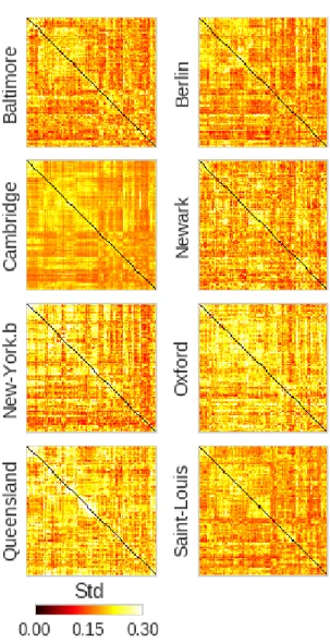
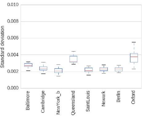
S1 DMN standard deviation of resting-state . . . 56

S2 Connectome standard deviation of resting-state . . . 57

S3 Standard deviation of resting-state . . . 58

S4 Homoscedasticity . . . 58

S5 Connectome variability across sites, motion effect . . . 59

S6 Connectome variability across sites, sex effect . . . 60

S7 Connectome variability across sites, age effect . . . 61

1 Correspondence between connectomes . . . 69

2 Classification findings . . . 71

2 Demeaned gray matter volume measures of the right hemisphere. Panel A shows individual maps and the correlation of every subject with all other subjects in Panel B. Panel C shows the subtypes templates representing subgroups in the dataset. Panel D shows the association of each individual map in A with the each subtype template in C. . . 82 3 Figure shows the precision, specificity and sensitivity of the three

modalities (fMRI, sMRI and fMRI+sMRI) at each stage (Base: basic classifier and HPS: highly predictive signature). Significant differences are shown with ∗ for p < 0.05 and ∗∗ for p < 0.001). . 83 4 Panel A shows the contribution of each modality to the decision,

the ratios are computed by the sum of the absolute coefficient for each modality. Panel B shows the coefficients of the high-confidence prediction model for each subtype map. Panel C shows, on top, the average maps for each modality and on the bottom the subtype maps used for the high-confidence prediction. . . 85 5 Statistic on the MCI showing the signature. Panel A shows the

percentage of MCI who progress to AD, the percentage of subjects positive for beta amyloid deposits using the AV45 marker and the percentage of carriers of one or two copies of the ApoE4 allele for the entire MCI cohort. Panel B shows the same statistics for the selection of the base classifier while Panel C displays statistics for subjects flagged as HPS. Panel D shows the clinical status of each HPS subject over time from the baseline scan. . . 88 6 Panel A shows the feature extraction method called subtypes weights,

Panel B framework workflow: stage 1 shows the hit probability computation based on random sub-sampling and stage 2 shows the training of dedicated classifier for each “high-confidence” sig-nature. Panel C shows the nested cross-validation scheme used in this method. . . 94

S1 Hit-probability distribution obtained from replicating the SVM train-ing 100 times from 80% of the traintrain-ing set. . . 100

LIST OF APPENDICES

Appendix I: First Appendix . . . xvi Appendix II: Second Appendix . . . xxxi Appendix III: Third Appendix . . . xlv

LIST OF ABBREVIATIONS

AD Alzheimer’s disease

BOLD Blood oxygen-level dependent CN Cognitively normal

CSF Cerebrospinal fluid CV Cross-validation

fMRI Functional magnetic resonance imaging GSC Global signal correction

HPC Highly predictable cases

IRM Imagerie par résonance magnétique MA Maladie d’Alzheimer

MCI Mild cognitive impairment MR Magnetic resonance

MRI Magnetic resonance imaging NIAK Neuroimaging analysis kit

PET Positron-emission tomography RS Resting-state

sMRI Structural magnetic resonance imaging SNR Signal to noise ratio

ACKNOWLEDGMENTS

My first contact with medical imaging research was 8 years ago at McGill University. I was captivated by the idea of using my technical knowledge to an important and stim-ulating field that is medicine. I was driven by the idea of helping patients and medical professionals to better understand and diagnose diseases at the individual level. During my studies as a Master student, I had the chance to collaborate with Dr. Pierre Bellec and he eventually convinced me to start a Ph.D. with him. Doing my Ph.D. was probably the best move I did... after asking my fiancé to marry me of course. Thank you so much, Pierre, for your support, guidance, great conversations and for giving me your love of research, I will be forever grateful. I would also like to thank my colleague’s from the lab past and present: Aman, Sebastian, Perrine, Yassine, Amal, PO, Jacke, Clara and Hien with whom I got a lot of great exchanges and fun. I would especially like to thank Pierre Orban and Angela for their great advice and support, your friendship and support defi-nitely made a difference. Thanks to the boys of the computer science department: Maor, Thomas, Francis, Cesar, Alexandre, Ishmael, I had extremely stimulating exchanges and ideas with you and I look forward to more of those in the future! Thanks also to my friends outside academia who kept me in a good mental state all those years and were so supportive.

Particular thanks to my parents and my brother Samuel for their great support through-out these years and through my academic endeavor. It has not always been easy but I made it through, thank you. Dad, your passion for science and research was probably the seed of my interest in that field. My in-laws: Isabel, Alain, and Guido who always believed in me and encouraged me to pursue my dreams.

Finally, I would like to give a very special thanks to the love of my life Bianca. Probably my greatest supporter and the one who always had faith in me and push me to surpass myself. Without you, I probably would have starved or eaten a very basic diet of ramens! You did all this even if you had to do your very own Ph.D. at the same time. I admire you...

CHAPTER 1

INTRODUCTION

1.1 General context

Machine learning is on a course to change the way clinical diagnoses are established and delivered. Supervised learning has historically needed large datasets to be able to perform well and unfortunately, this is a scarce resource in medical imaging. One solu-tion to increase the sample size is to aggregate data from heterogeneous sources, with the downside of adding more variance in the dataset. Another source of variance that can impact the performance of an inference model is the imperfect knowledge of clinical diagnoses, reflected in the labels used for training and evaluating our models. Clini-cal diagnoses are often incorrect, incomplete or not specific enough to the variants that exist in the pathophysiology within a given disorder. Heterogeneous data sources and heterogeneous clinical labels are two issues particularly prevalent in the diagnosis and prognosis of Alzheimer’s disease (AD) using magnetic resonance imaging (MRI), which is the main application of my doctoral work.

The number of Canadians suffering from AD is rapidly increasing, with tremen-dous social and economic impact. Despite the emergence of promising drugs, the recent clinical trials with demented patients have failed. Dementia comes very late in the devel-opment of the disease, at a stage where the degeneration of neural tissues has likely gone beyond repair. In order to be efficient, therapies should be initiated in the decades predat-ing dementia, in a preclinical stage where patients experience no or very mild symptoms (see chapter 1.2). There is, unfortunately, no accurate biomarker(s) that can predict AD in this preclinical stage, and that could help identify the individuals that would progress to dementia and benefit from such interventions. It would also be useful to identify pre-symptomatic markers of the disease in order to understand the underlying mechanism of the pathology. Promising early AD biomarkers can be captured using MRI, which is a broadly available and noninvasive technique. Two separate modalities have been shown

to be of great interest in the investigation of the disease progression, namely structural MRI - that can give information on brain atrophy patterns - and functional MRI - that investigates functional interactions between various brain structures - (see chapter 1.3). Generation of biomarkers require a complex process of data preparation: preprocessing (denoising and spatial alignment) (see chapter 1.4) and features extraction. A standard way to extract meaningful information from the rich 4D images provided by fMRI is to use resting-state connectivity measures and is detailed in chapter 1.5. Different practices like scientific consortia, data sharing and open clinical trials have emerged, and all de-liver large public and multisite datasets which can be used to discover new biomarkers (see chapter 1.6). Unfortunately, the gain in sample size due to data aggregation across sites comes at the price of increased heterogeneity (see chapter 1.7.3.1 and 1.7.3.2) and may impact the discriminative properties of our markers.

In addition, heterogeneity also exists in the clinical labels (Drysdale et al. 2017) (see chapter 1.7.3.3). The last point could drastically affect the ability of a prediction model to converge to a solution that will effectively predict clinical labels. Finally I will outline the objectives and contributions of my Ph.D. thesis to deal with technical and clinical sources of heterogeneity in section 1.8.

1.2 Alzheimer’s disease

Alzheimer’s disease (AD) is a major neurodegenerative disorder characterized by the accumulation of beta amyloid plaques and tau neurofibrillary tangles in the brain. AD gradually destroys a patient’s memory and ability to reason, make judgments, com-municate and carry out daily activities (Jeong 2004). With the aging of the population worldwide, this disorder has attracted much attention. Evidence from elderly individuals suggests that the pathophysiological process of AD begins years, if not decades, before the diagnosis of clinical dementia (Morris 2005). The clinical disease stages of AD are divided into three phases described by Jack and colleagues Jack et al. (2010).

First is a pre-symptomatic phase in which individuals are cognitively normal but some have pathological changes in AD. Second is a prodromal phase of AD, commonly

referred to as mild cognitive impairment (MCI) (Petersen 2004), which is characterized by the onset of the earliest cognitive symptoms (typically deficits in episodic memory) that do not meet the criteria for dementia. The severity of cognitive impairment in the MCI phase of AD varies from an early manifestation of memory dysfunction to more widespread dysfunction in other cognitive domains. The final phase in the evolution of AD is dementia, defined as multi-domain impairments that are severe enough to result in loss of function(Jack et al. 2010).

The use of a biomarker for the early diagnosis of pathologies has a long history, with many studies showing the feasibility of using an AD biomarker to predict conver-sion from MCI to AD. These studies show that individuals in the course of developing AD can be identified earlier in the course of the disease by using the MCI stage with the addition of imaging and cerebrospinal fluid (CSF) biomarkers to enhance diagnostic specificity (Chetelat et al. 2003, Jack et al. 1999, Mattsson et al. 2009, Yuan et al. 2009). It could be possible to diagnose AD after the exclusion of other forms of dementia, al-though a formal diagnosis can currently only be made after a post-mortem evaluation of the brain tissue (McKhann et al. 1984). This is one of the reasons why MRI based analysis and diagnostic tools are currently undergoing intense study in clinical neuro-science research. The early prediction of disease onset is also needed for clinical trials investigating disease-modifying therapies, since treatment of patients with no or mild symptoms are more likely to have a positive outcome, compared to demented subjects who may have such extensive damage that it may be too late to modify the trajectory of the disease.

The current dominant hypothesis in the field for the chain of events in AD patho-physiology is the β -amyloid (Aβ )-cascade. It suggests that interstitial Aβ proteins exert a toxic effect on surrounding neurons and synapses by forming plaques, thereby dis-turbing their function (Hardy and Selkoe 2002, Shankar et al. 2008). Moreover, a recent research study suggests that, prior to neuronal death resulting in brain atrophy, disruption of functional connectivity may arise in response to an unknown systemic problem and represent an early outcome of Aβ protein plaque formation in AD (Sheline and Raichle 2013). Atrophy is the result of neuronal death and is measured in vivo using structural

MRI measuring the thickness of the gray matter of the cortex (also called cortical thick-ness) or the gray matter volume in various parcels of the brain. Already in the stage preceding aggregation of Aβ fragments into amyloid plaques, there is a dysfunction of synaptic transmission in many brain regions due to dimers and monomers from the Aβ cascade (D’Amelio and Rossini 2012). As illustrated in Sperling et al. (2011) a viable hypothesis is that functional changes precede the structural changes as well as clinical symptoms and are believed to start in the preclinical phase of the disease. A multimodal combination of structural and functional information may, therefore, lead to accurate predictions of individual clinical trajectories.

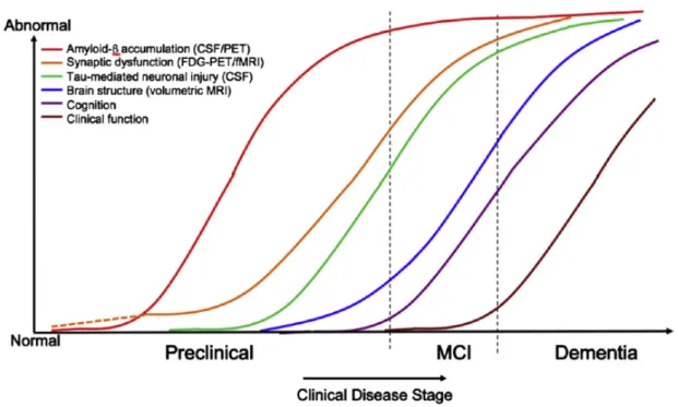
Figure 1.1: Hypothetical model of dynamic biomarkers of the AD expanded to explain the preclinical phase: Aβ as identified by cerebrospinal fluid Aβ 42 assays or PET amy-loid imaging. Synaptic dysfunction evidenced by fluorodeoxyglucose (F18) positron emission tomography (FDG-PET) or functional magnetic resonance imaging (fMRI), with a dashed line to indicate that synaptic dysfunction may be detectable in carriers of the ε4 alleles of the apolipoprotein E gene before detectable Aβ deposition. Neuronal injury is evidenced by cerebrospinal fluid tau or phospho-tau, and brain structure is ev-idenced by structural magnetic resonance imaging. Biomarkers change from normal to maximally abnormal (y-axis) as a function of disease stage (x-axis). The temporal trajec-tory of two key indicators used to stage the disease clinically, cognitive and behavioral measures, and clinical function is also illustrated. Figure from Sperling et al. (2011).

1.3 Overview of magnetic resonance imaging

1.3.1 Overview of structural magnetic resonance imaging

Structural magnetic resonance imaging (sMRI) also called anatomical MRI is an imaging technique that provides static anatomical information. Some atomic nuclei are

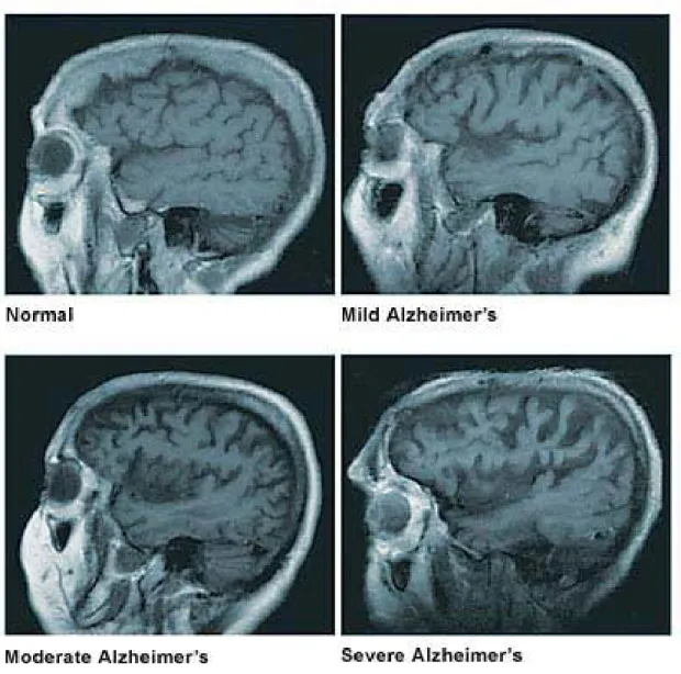
able to absorb and emit radio frequency energy when placed in an external magnetic field. In clinical and research MRI, hydrogen atoms are most often used to generate a detectable radio-frequency signal that is received by antennas in close proximity to the head. Hydrogen atoms exist naturally in mammals and in abundance, particularly in wa-ter and fat. For this reason, most of the structural MRI sequences essentially map the location of water and fat in the body. Pulses of radio waves excite the nuclear spin of the hydrogen atoms to determine the hydrogen concentration (a proxy for water concentra-tion), and magnetic field gradients are used to localize the signal in space by encoding the radio frequency in space. By varying the parameters of the pulse sequence, different contrasts may be generated between tissues based on the relaxation properties of the hy-drogen atoms. The main two contrasts used are T 1− and T 2− weighted imaging. This imaging modality is widely used in hospitals and clinics for medical diagnosis, staging of disease using brain atrophy (see Figure 1.2) and follow-up without exposing the body to ionizing radiation.

Figure 1.2: The figure for brain atrophy at four stages of AD pathology. Figure from Mayo fondation1

1.3.2 Overview of functional magnetic resonance imaging

In functional magnetic resonance imaging (fMRI), the acquisition process is slightly different than for the anatomical MRI acquisition. fMRI uses the principle of the relax-ation of hydrogen nuclei, by using specific fMRI sequences of T 2∗ weighted

acquisi-tions that are sensitive to local distoracquisi-tions of the magnetic field. Deoxyhemoglobin, a form of hemoglobin without oxygen, will create such local distortions of the magnetic field, since it is a paramagnetic molecule (positive magnetic susceptibility) (Ogawa et al. 1990). The data acquired using fMRI rely on the hypothesis that areas showing de-creased deoxyhemoglobin concentration are due to sustained brain activity. Following neuronal activity, neurons require energy to restore the electrical and ionic concentra-tion balance across the cell membrane. The main mechanism to generate this energy is glucose oxidative metabolism, which requires the delivery of oxygen and glucose by the blood to the site where brain activity takes place (Ogawa et al. 1990). Initially, fMRI was thought to be a good technique to measure the cerebral metabolic rate of oxygen, since the new blood rushing in causes a proportional effect on the venous-end, resulting in a decrease in deoxyhemoglobin concentration, and thus an increase in fMRI signal. The concentration of deoxyhemoglobin actually depends mainly on three factors or phe-nomena: the metabolic rate of oxygen consumption, cerebral blood volume and cerebral blood flow (Hoge et al. 1999). As a result, the fMRI signal is the outcome of competing effects following neuronal activity.

Figure 1.3: Representation of the brain and its vasculature (on the left) and a schematic view of the interaction between the effect of neuronal activity on local changes in blood oxygenation signal (BOLD) (on the right) (adapted from Heeger and Ress (2002)).

1.4 Preprocessing

Normalization of the data is crucial to obtain a consistent and accurate classifier (Kotsiantis 2007). Therefore particular attention is placed on the correction and normal-ization procedure applied to the rs-fMRI data used in this study. A series of standard preprocessing steps is usually applied in an attempt to correct for various artifacts that would perturb the subsequent analysis and to align the brains of different individuals. The BOLD effect associated with neuronal activity generally results in a relatively small fluctuation of the MR signal. Many factors can influence this signal. Among them, the physiological activity associated mainly with respiration, cardiac pulsations, and pa-tient’s motion are major contributors to the noise and are spatially spread everywhere within the brain volume. These sources of noise result in large correlations between BOLD signals of distant voxels. Another factor is the fact that we need a form of spatial normalization of the individual brains in order to perform analysis across subjects (due to anatomical variance among subjects). This spatial normalization (coregistration of the individual brains with a reference template) is necessary but can potentially be another source of confound.

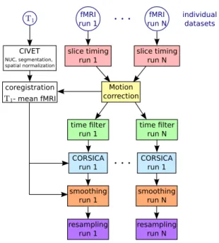
Therefore, preprocessing methods were designed in an attempt to remove specifically the so-called structured noise and motion artifacts from the raw fMRI data. A schematic representation of the preprocessing pipeline can be seen in Figure 1.4.

Figure 1.4: Schematic of the preprocessing pipeline including spatial and functional normalization (NIAK preprocessing pipeline2).

The basic steps are as follows: (1) correction for slice timing differences due to delay in acquisition sampling; (2) rigid-body motion estimation for within and between runs. Motion correction operates by selecting one functional volume as a reference to align all other functional volumes. Most head motion algorithms describe head movement by 6 parameters, three translation parameters (displacement) and three rotation param-eters and are sufficient to characterize the motion of rigid bodies (see Figure 1.5); (3) Coregistration of the functional data in a reference space; (4) resampling of the func-tional data in the stereotaxic space (references brain used as a common space between subjects); (5) regression of confounds in order to remove spatially structured noise from the fMRI time-series. The confounds are the slow time drift, the high-frequency noise signal, motion parameters, the average signal white matter as well as the average signal of the ventricles (containing cerebrospinal fluid CSF a frequent source of noise and ar-tifact). Some groups have suggested that these corrections are not sufficient to remove motion artefacts and propose some additional corrective procedure (detailed in Chapter 2); and (6) the spatial smoothing is usually applied using a Gaussian blurring kernel to

improve signal to noise ratio (SNR), improve validity of the statistical tests by making the error distribution more normal and finally reduce anatomical and functional varia-tions between subjects (Mikl et al. 2008, Worsley and Friston 1995).

Neuroimaging Analysis Kit – NIAK – user’s guide The fMRI preprocessing pipeline

Pipeline options

Motion correction I

Figure 1.5: Motion estimation based on rigid-body motion estimation of the functional volumes, the procedure provides 6 motion parameters for each volume (3 translation and 3 rotation) Schematic of the preprocessing pipeline including spatial and functional normalization (from NIAK preprocessing pipeline3).

1.5 Resting-state connectivity

Resting-state (RS) functional connectivity captures the spatial coherence of slow fluctuations in hemodynamic temporal activity, without performing a prescribed task, as opposed to the task-based acquisition where the subject has to perform a specific task. In resting-state acquisition, the subject is instructed to rest with his eyes open or closed. These temporal fluctuations can be monitored using the signal measured with fMRI. The first study that introduced the concept of resting state functional connectivity was the one of Biswal et al. (1995). They considered the left primary sensorimotor cortex as a seed region for an analysis in a resting-state condition. This analysis consisted in calculating the temporal correlation between the signal of the seed area and the time course of all the voxels of the brain. They found RS correlations between brain regions known to be involved in sensorimotor function. A more recent review done by Fox and Raichle

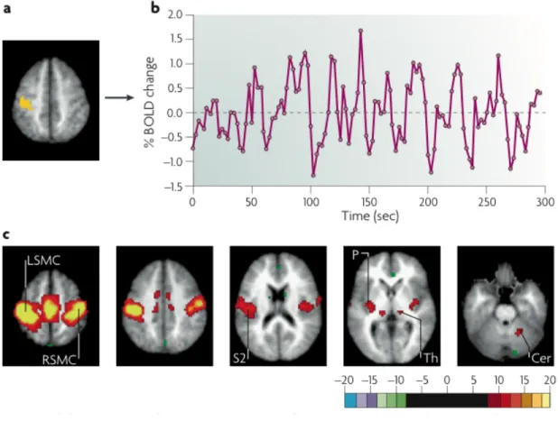
(2007) illustrated in Figure 1.6 shows the ability to identify the complete sensorimotor network using only the BOLD signal from a small region of that network.

Figure 1.6: Generation of resting-state correlation maps. a) Seed region in the left so-matomotor cortex (LSMC) is shown in yellow. b) Time course of spontaneous blood oxygen level dependent (BOLD) activity recorded during resting fixation and extracted from the seed region. c) Statistical z-score map showing voxels that are significantly cor-related with the extracted time course. Their significance was assessed using a random effects analysis across a population of ten subjects. In addition to correlations with the right somatomotor cortex (RSMC) and medial motor areas, correlations are observed with the secondary somatosensory association cortex (S2), the posterior nuclei of the thalamus (Th), putamen (P) and cerebellum (Cer) (Fox and Raichle 2007).

These early results from Biswal et al. suggest that it is possible to identify the func-tional organization of different structures without doing any specific task, just by looking at spontaneous fluctuations in brain activity. Several studies have demonstrated that

pat-terns extracted from temporal correlations of RS signals within the brain volume are organized in space and have a good reproducibility from subject to subject (Damoiseaux et al. 2006, Dansereau et al. 2014). Each network is a combination of multiple brain regions or units, not necessarily spatially close to each other, which share similar low frequency fluctuations of the BOLD signal. This information is usually represented as a functional connectivity matrix where one column of the matrix represents the connec-tivity of a region or network with the rest of the brain called a functional connecconnec-tivity map (see Figure 1.7). These networks show the functional organization of various brain regions (see Figure 1.8 for a list of common RS networks).

Figure 1.7: Functional connectome: on the left a representation of a functional parcel-lation, in the middle a region-level functional connectome representing the connectivity between each pair of region, and on the right the connectivity map based on a region of interest extracted from the functional connectome.

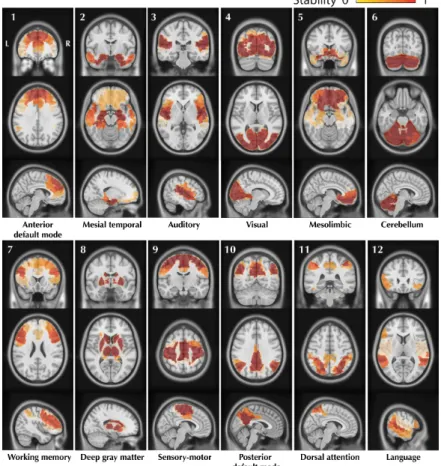
Figure 1.8: The figure shows 12 RS networks identified using a BASC (Bootstrap Anal-ysis of Stable Cluster (Bellec et al. 2010b)) group level analAnal-ysis of 25 healthy control subjects. BASC is a clustering based method using evidence accumulation for the identi-fication of stable clusters. For each network: 3 slices (coronal, axial, sagittal) are shown superimposed on an anatomical MRI template (MNI152). Labelling of each network was done visually based on previously reported intrinsic networks in the literature. The fig-ure shows networks typically reported in the litteratfig-ure: Default Mode Network (#1,#10), Auditory (#3), Visual (#4), Sensory-Motor (#9), Attention (#7,#11) and Language(#12). BASC also identified 4 other networks, less often reported, but characterized by high statistical stability: Mesio-Temporal (#2), Mesolimbic (#5), Cerebellum (#6) and Deep Gray Matter (#8) (Dansereau et al. 2014).

Interestingly, RS fMRI signals have also been used for the diagnosis of some neuro-logical and psychiatric disorders, such as multiple sclerosis (Lowe et al. 2002), epilepsy (Waites et al. 2006), schizophrenia (Liang et al. 2006, Salvador et al. 2007, Zhou et al. 2007; 2008), attention deficit hyperactivity disorder (Tian et al. 2007, Zang et al. 2007),

blindness (Liu et al. 2007, Yu et al. 2007), major depression (Anand et al. 2005, Gre-icius et al. 2007) and acute brainstem ischemia (Salvador et al. 2005). We believe that resting-state fMRI will be an increasingly important modality for exploring the func-tional abnormalities of patients with AD (Buckley et al. 2017) since we would like to identify signs of the pathology prior to major atrophy or cognitive decline. Therefore functional alterations and/or compensation are believed to occur earlier in the disease progression justifying the use of this modality for early detection of AD pathology.

1.6 Multisite

Quality and quantity of data are usually the main factors that influence the ability of a model to do good inferences. The quantity of data can be expanded through data aggre-gation, hence why an increasing number of large publicly available cohorts of subjects has emerged, like the 1000 functional connectome (Biswal et al. 2010), ADNI (Mueller et al. 2005), and ABIDE (Di Martino et al. 2014), among others (see Woo et al. (2017) Table 1 for a more exhaustive list). In a clinical trial, the justification for multisite ac-quisition is more of a logistical one than a financial reason; they need to recruit a large amount of subjects in a short period of time. In order to achieve this goal, they man-date the recruitment to multiple clinical centers across the globe which accelerates the evaluation time of a drug. Although these centers may have been harmonized by their scanner protocols, scanners will have differences in their software version, the specific add-on to the scanners, and, most importantly, vendors (even field strength may differ in some cases). Unfortunately, between studies, MR acquisition methodologies are among the most commonly cited sources of measurement variation (Friedman et al. 2006). This is why it is important to assess if multisite resting-state connectivity analysis is feasible: Can we combine the data from multiple sources while still detecting effects of interest in the data? What corrective measure on the data should be applied to reduce the bias introduced by multisite data collection? Among the factors of variability across sites, we can list the following 3 categories described in (Yan et al. 2013b):

1. Acquisition-related variations:

(a) Scanner make and model (Friedman et al. 2006)

(b) Sequence type (spiral vs. echo planar; single-echo vs. multi-echo) (Klarhofer et al. 2002), parallel vs. conventional acquisition (Feinberg et al. 2010) (Lin et al. 2005)

(c) Coil type (surface vs. volume, number of channels, orientation).

(d) Acquisition parameters: repetition time, number of repetitions, flip angle, echo time, and acquisition volume (field of view, voxel size, slice thickness/-gaps, slice prescription) (Friedman and Glover 2006).

2. Experimental-related variations:

(a) Participant instructions (Hartstra et al. 2011), eyes-open/eyes-closed (Yan et al. 2009) (Yang et al. 2007), visual displays, experiment duration (Fang et al. 2007) (Van Dijk et al. 2010).

3. Environment-related variations:

(a) Sound attenuation measures (Cho et al. 1998) (Elliott et al. 1999).

(b) Attempts to improve participant comfort during scans (e.g., music, videos) (Cullen et al. 2009).

(c) Head-motion restraint techniques (e.g., vacuum pad, foam pad, bite-bar, plaster cast head holder) (Edward et al. 2000) (Menon et al. 1997).

(d) Room temperature and moisture (Vanhoutte et al. 2006).

In 2009, the 1000 Functional Connectomes Project (FCP) released a sample of 1200+ fMRI scans collected at 33 different institutions, which provided a glimpse of the vari-ability in imaging characteristics employed by the neuroimaging field. The parame-ters of the imaging acquisition varied across sites, while the majority of subject-related variables are not reported (due in most cases, to the fact that they were not thoroughly

recorded). Despite justifiable skepticism, feasibility analyses demonstrated that mean-ingful explorations of the aggregated dataset could be performed (Biswal et al. 2010). Although no explicit correction for multisite variability was used, they only used a global signal correction (GSC) to normalize subjects which may introduce anti-correlations in the data (Carbonell et al. 2014, Fox et al. 2009, Murphy et al. 2009, Power et al. 2014, Saad et al. 2012). After accounting for site-related differences, the analysis showed brain-behavior relationships with variables such as age, gender, and diagnostic label, and confirmed a variety of prior hypotheses (Biswal et al. 2010, Fair et al. 2012, Tomasi and Volkow 2010, Zuo et al. 2012). While encouraging, it remains a source of concern if unharmonized datasets can be aggregated together since many uncontrolled and un-known factors in the 1000 FCP, may be adding variance unrelated to simple site effects as highlighted by Yan et al. (2013a). Another demonstration of substantial multisite variance is the study reported by Nielsen et al. (2013) where the authors compared a monosite and a multisite dataset of subjects with autism and concluded that the multisite classification accuracy was much lower for multisite than monosite (Nielsen et al. 2013).

1.7 Prediction of clinical diagnosis using medical images 1.7.1 Prediction in the context of AD

In the past few years, several major studies have been initiated that have aimed to predict who will develop AD dementia at the prodromal or even asymptomatic stages, with the ultimate goal of providing a platform for interventions with disease-modifying therapies. Many of these studies were designed to evaluate the role of neuroimaging and clinical biomarkers in assessing and predicting progression in individuals without cognitive impairment and in individuals with MCI.

A recent body of literature has focussed on the classification of subjects at various stages of AD and progression from a prodromal stage to AD dementia using one of the various brain imaging modalities available, including positron emission tomogra-phy (PET) imaging (Cabral et al. 2015, Mathotaarachchi et al. 2017), structural MRI (Adaszewski et al. 2013, Eskildsen et al. 2013, Liu et al. 2015; 2013, Misra et al. 2009,

Salvatore et al. 2015), and functional MRI Challis et al. (2015), Chen et al. (2011), Jie et al. (2014), Khazaee et al. (2015), see (Rathore et al. 2017) for a complete review. More recently some groups used multimodal data from the ADNI dataset to improve prediction accuracy and reported classification performance of the order of 95% accu-racy to classify patients with AD dementia vs. CN (Xu et al. 2015, Zhu et al. 2014, Zu et al. 2016) and 80% accuracy to identify patients with MCI who will progress to AD dementia (Cheng et al. 2015a;b, Korolev et al. 2016, Moradi et al. 2015).

1.7.2 Cross-validation

As machine learning algorithms are increasingly used to support clinical decision making, it is important to reliably quantify how a prediction model will generalize to an independent dataset or site. Cross-validation (CV) is the standard approach for eval-uating the accuracy of such algorithms. Validation is the task of training the data on a subset of the data and evaluating its performance on the hold-out portion that has never been seen by the model. Cross-validation, on the other hand, is the repeated measure of the validation with non-overlapping subsamples. Multiple CV methods exist and, de-pending on the end goal, some may be better than others to obtain an unbiased estimate of the model accuracy as reported by (Saeb et al. 2016) where they compared two pop-ular CV methods: record-wise and subject-wise cross-validation. In their paper, Saeb and colleagues made the case that record-wise CV leads to overestimated accuracy score that does not reflect the true prediction accuracy when evaluated on unseen subjects. As highlighted by Little et al. (2017), Varoquaux (2017) the context and question that we want to answer will determine the optimal CV scheme.

1.7.3 Dealing with heterogeneity

Accounting for heterogeneous sources of variance is important since they may reduce the predictive potential of our model.

1.7.3.1 Feasibility of multisite studies

In order to extract good and reliable biomarkers most machine-learning models re-quire large sample sizes. Neuroimaging analysis is typically being acre-quired on one sin-gle site with the same device. The major limitations of this type of recruitment scheme is the decimation of small samples (small datasets acquired in parallel with different protocols on different scanners that increase the number of studies but not the sample size) and the difficulty to recruit a large amount of participants in the same location in a reasonable time frame as mentioned previously in the multisite section. A solution for the previously mentioned issues is to aggregate data from multiple sites into one large dataset. As referenced earlier, data aggregation poses a number of difficulties due to the added variability incurred by pooling multiple data from multiple sources. The ques-tion is: does the tradeoff of having a larger sample supersede the added heterogeneity obtained by aggregating multiple sites into one large dataset?

As indicated earlier, the problem regarding multisite heterogeneity can easily be transposed to a more general problem in machine learning related to the aggregation of various datasets that were not obtained with the same equipment and standards e.g. pictures taken with various digital camera brands of a diverse range of quality and where all picture labels are not uniformly distributed across cameras (Deng et al. 2009). Given sufficient data and a model with enough capacity, this variability can be modeled. We, unfortunately, do not have enough data (the data is very scarce and expensive to acquire) to fully model this variability in medical imaging applications. The lack of ground truth to evaluate the performance of a model in various training configurations and misdiagno-sis may affect our ability to evaluate the variance contribution of a multisite acquisition. We, therefore, need to evaluate the detrimental effect of the aggregation of data on our in-ference models, compared to the standard monosite analysis, using realistic simulations and this is precisely what we propose to do in the context of fMRI data analysis.

1.7.3.2 Generalizability of models: Harnessing heterogeneity

In order to be useful, biomarkers that are identified on one dataset need to be gener-alizable to other datasets. A standard approach to estimate the performance of a given prediction model on unseen samples is to do cross-validation. This is very well known principle in the machine learning community and a standard step in the evaluation of a prediction model (Friedman et al. 2001). Now let us assume that our data is collected using multiple sources (e.g. recording devices). Multiple scenarios are possible, so we could use only the data coming from one device and do the cross-validation for that dataset to obtain an accuracy score. This accuracy score will reflect the performance of the model for data coming from that specific device but does not give any idea of the performance of the model for data coming from a different device. The same problem can be directly applied in neuroimaging where the dataset is obtained from MRI scan-ners that may have different properties and site specific characteristics. A lot of the early work on pathology prediction in neuroimaging has reported an accuracy score where the training and test data came from the same scanner (Arbabshirani et al. 2017, Costafreda et al. 2009, Fan et al. 2005, Fu et al. 2008, Hahn et al. 2011, Kawasaki et al. 2007, Lao et al. 2004, Marquand et al. 2008, Mourao-Miranda et al. 2005, Nouretdinov et al. 2011, Rathore et al. 2017). Unfortunately, more recent work has shown that the accuracy drops dramatically when the model is applied to another independent dataset (Abraham et al. 2016, Cheng et al. 2015c, Schilbach et al. 2016, Skåtun et al. 2016, Woo et al. 2017). It is therefore important to evaluate if this behavior was due to a lack of information at training, rendering the model to be unable to generalize well to independent devices and sites. In order to explore this question, it is possible to use various sampling strategies to evaluate if the pooling of multiple sites at training yields a better generalization outcome for unseen data. This is particularly important for clinical use since the predictive model will most likely be used with data obtained from a different site than the site(s) used for training and accuracy evaluation. We, therefore, need a less biased accuracy estimate that will correctly quantify the generalizability of the model in unseen sites. The site het-erogeneity needs to be learned while training the model so that the model can become

invariant to it.

1.7.3.3 Clinical label heterogeneity

Heterogeneity can appear in different forms and at different levels, for example, we can have acquisition heterogeneity due to: recruitment bias, the use of different scan-ners, software to process the data, interindividual biological differences or any sort of acquisition noise present in the data. Those types of heterogeneity, mainly explained in the previous sections (section 1.7.3.2, and 1.7.3.2), reduce the effect size and therefore may need to be modeled as much as possible to reduce their impact. Another source of heterogeneity is the labels heterogeneity. By labels heterogeneity, we mean that they are not precise enough to encompass the underlying variability of the data or that some sub groups are underrepresented.

This other source of heterogeneity is well established in the clinical world but is usually not accounted for until recently in the machine learning world applied to medical problems. In an ideal scenario you would have multiple sub-diseases in a dataset with a large number of examples of each sub category. In that context the algorithm would learn to identify what is common among all of those subjects even if they have drastically different underlying causes. Unfortunately, in most clinical datasets we are far from unlimited data and a subgroup may be under-represented or simply not identified in some cases, crippling the ability of the model to do its job correctly. The fact that the labels are poorly defined renders the task of a perfect prediction virtually impossible since it is ill posed from the start. We basically have imposed overly strict and sometimes subjective categorical labels to disorders like schizophrenia Insel (2010) (that is more seen as a spectrum disorder) or Alzheimer’s disease that encompasses multiple sub-forms of the disease (Lam et al. 2013) and/or mixed pathologies.

Since clinical diagnoses are often incorrect, incomplete or not specific enough to the variants that exist in the pathophysiology, it will impair our ability to have true gold standard labels and inevitably the prediction model will be affected by this lack of pre-cision in the clinical labels. For example Beach et al. (2012) have shown that a clinical error in diagnosis for AD dementia exists after post-mortem neuropathological

inves-tigation revealed that only 70.9% to 87.3% (depending on the clinical criteria) of the probable AD subjects were diagnosed correctly. Beach and colleagues also found that a range between 44.3% to 70.8% (depending on the clinical criteria) of the subjects diag-nosed as non-AD had, in fact, AD pathology, as defined by post-mortem histopathologic evaluations. Data-driven analysis of sMRI in AD further showed that symptomatic het-erogeneity is related to different patterns of atrophy spreading in AD (Dong et al. 2016, Zhang et al. 2016). Recently, Dong et al. (2016) also reported multiple subtypes of dysconnectivity in patients suffering from AD dementia, MCI, and subjective cognitive impairment, using diffusion magnetic resonance imaging, and reported associations be-tween subtypes and the severity of cognitive impairment. These findings highlight the existence of a great heterogeneity in the signature of AD pathology.

Most classification models propose a built-in confidence estimate over their predic-tion. Unfortunately, it is possible for a model to be very confident about a prediction that is completely wrong (Niculescu-Mizil and Caruana 2005) this can be true with outliers for example or in over-fitting scenarios (Waterhouse et al. 1996). This is mainly due to the way confidence is calculated, namely the distance of that sample to the hyperplane. To deal with outliers a field of statistics called robust statistic has emerged to focus on that particular issue and render the model to be robust to outliers. Outliers, by definition, usually represent a very small fraction of the examples, and it is precisely in those con-ditions that the robust statistic holds (Black and Rangarajan 1996). In our case, although we have a heterogeneous population, there is no guarantee that a majority of the subjects are homogeneous, rendering this type of solution unhelpful. The parametric estimation of the model confidence probability that was proposed by Platt et al. (1999), Wu et al. (2004) is limited by strong a priori on the data. We would therefore benefit from a non-parametric metric that could compute the likelihood of a subject to be correctly classified and use that to identify a highly predictable subgroup of subjects.

The label heterogeneity could be better modeled with a very large dataset encom-passing most of the labels’ variability. This would help in part to refine clinical labels based on groups of individuals who share a common phenotypic signature and better model the intersubject variability. Unfortunately, such large datasets do not exist yet but

may arise in the future. In the meantime what can be done with the existing datasets? Would it be possible to extract meaningful information that can be used in a clinical setup even though they encompass heterogeneous clinical labels?

I propose this approach in the context of AD clinical trial enrichment, but the issue raised is general and touches many machine learning applications. Any high-risk prob-lem where some specific action is very impactful or costly, and the lack of action has a small cost, is relevant. One would want to only implement those actions in the cases where the positive outcome is highly probable. For example, when trading stocks, we would like to place an order to buy or sell a stock only when it is highly probable that the stock will rise or fall in the next time point instead of placing a bet at each time point.

The first part of my scientific contributions is related to realistic multisite simulation and generalizability, and I have proposed a domain specific solution to a general prob-lem. For the second part related to the problem of labels heterogeneity, I have proposed a generic solution to a domain specific problem. Since this solution is generic it could be used in a variety of other domains.

1.8 Objectives

The overall objective of this thesis was to explore the impact of heterogeneity in its various forms on imaging analysis and corrective approaches that can be used to reduce its impact. We mainly focus on two aspects of variance, namely the multisite aggregation and the clinical labels heterogeneity.

1.8.1 First paper objectives

The first contribution of this thesis (Dansereau et al. (2017)) addressed the feasibility and impact of multisite fMRI analysis in standard univariate or multivariate machine learning experiments. This question is very important since it is an emerging strategy to increase sample size and is gaining a lot of interest in the neuroimaging community. Since we lack a ground truth where we have the exact same effect and subjects scanned using a monosite and a multisite scenario, the objective was to use realistic simulations

to generate an equivalent dataset.

1.8.2 Second paper objectives

The second paper’s objective (Orban et al. (2017a)) was to explore the generaliz-ability of various training schemes (monosite CV, intra-sites CV, inter-sites CV) in the context of a multisite dataset to identify if a bias exists in the reported accuracy perfor-mance. We also aimed to determine the most unbiased strategy to estimate the general-izability performance of a model on true unseen data coming from a different site. Our hypothesis was that even though a multisite acquisition may increase the heterogeneity of the dataset, it is useful to test the generalizability of the results across different sam-ples, making it more likely to obtain generalizable features reflecting generic traits of the pathology rather than particularities of a single dataset. To do so we evaluated the effect of intra-site vs. inter-site training on prediction accuracy performance using real data from a clinical population acquired on different sites instead of simulated effects of pathology like we did in my preceding work.

1.8.3 Third paper objectives

The heterogeneity in clinical labels has to our knowledge not been previously ad-dressed even though it is well-known in the clinical community that diseases like AD may encompass multiple sub diseases that are currently not diagnosed or identified as such. The main problems are the comorbid factors and mismatch between pathological and clinical stages that may cause heterogeneity in the clinical labels. We, therefore, proposed in the third paper to design a prediction pipeline for the data-driven identifica-tion of a signature of AD that will account for the heterogeneity of labels and improve the prediction accuracy on a subset of the population. We will also evaluated if that signature can be found in a prodromal stage of the disease (MCI) and if it could be a reliable marker of progression to AD dementia.

CHAPTER 2

STATISTICAL POWER AND PREDICTION ACCURACY IN MULTISITE RESTING-STATE FMRI CONNECTIVITY

Published in Neuroimage. 20171

C. Dansereau, Y. Benhajali, C. Risterucci, E. Merlo Pich, P. Orban, D. Arnold, P. Bellec

2.1 Abstract

Connectivity studies using resting-state functional magnetic resonance imaging are increasingly pooling data acquired at multiple sites. While this may allow investigators to speed up recruitment or increase sample size, multisite studies also potentially intro-duce systematic biases in connectivity measures across sites. In this work, we measure the inter-site effect in connectivity and its impact on our ability to detect individual and group differences. Our study was based on real, as opposed to simulated, multisite fMRI datasets collected in N = 345 young, healthy subjects across 8 scanning sites with 3T scanners and heterogeneous scanning protocols, drawn from the 1000 functional connec-tome project. We first empirically show that typical functional networks were reliably found at the group level in all sites, and that the amplitude of the inter-site effects was small to moderate, with a Cohen’s effect size below 0.5 on average across brain connec-tions. We then implemented a series of Monte-Carlo simulations, based on real data, to evaluate the impact of the multisite effects on detection power in statistical tests com-paring two groups (with and without the effect) using a general linear model, as well as on the prediction of group labels with a support-vector machine. As a reference, we also implemented the same simulations with fMRI data collected at a single site using an identical sample size. Simulations revealed that using data from heterogeneous sites

only slightly decreased our ability to detect changes compared to a monosite study with the GLM, and had a greater impact on prediction accuracy. However, the deleterious effect of multisite data pooling tended to decrease as the total sample size increased, to a point where differences between monosite and multisite simulations were small with N= 120 subjects. Taken together, our results support the feasibility of multisite studies in rs-fMRI provided the sample size is large enough.

Highlights

• Small to moderate systematic site effects in fMRI connectivity.

• Small impact of site effects on the detection of group differences for sample size > 100.

• Linear regression of the sites prior to multivariate prediction do not improve pre-diction accuracy.

2.2 Introduction 2.2.1 Main objective

Multisite studies are becoming increasingly common in resting-state functional mag-netic resonance imaging (rs-fMRI). In particular, some consortia have retrospectively pooled rs-fMRI data from multiple independent studies comparing clinical cohorts with control groups, e.g. normal controls in the 1000 functional connectome project (FCP) (Biswal et al. 2010), children and adolescents suffering from attention deficit hyperac-tivity disorder from the ADHD200 (Fair et al. 2012, Milham et al. 2012), individuals diagnosed with autism spectrum disorder in ABIDE (Nielsen et al. 2013), individuals suffering from schizophrenia (Cheng et al. 2015c), or elderly subjects suffering from mild cognitive impairment (Tam et al. 2015). The rationale behind such initiatives is to dramatically increase the sample size at the cost of decreased sample homogeneity. The systematic variations of connectivity measures derived using different scanners, called

site effects, may decrease the statistical power of group comparisons, and somewhat mit-igate the benefits of having a large sample size (Brown et al. 2011, Jovicich et al. 2016). In this work, our main objective was to quantitatively assess the impact of site effects on group comparisons in rs-fMRI connectivity.

2.2.2 Group comparison in rs-fMRI connectivity

In this work, we focused on the most common measure of individual functional con-nectivity, which is the Pearson’s correlation coefficient between the average rs-fMRI time series of two brain regions. To compare two groups, a general linear model (GLM) is typically used to establish the statistical significance of the difference in average con-nectivity between the groups. Finally a p-value is generated for each connection to quantify the probability that the difference in average connectivity is significantly dif-ferent from zero (Worsley and Friston 1995, Yan et al. 2013b). If the estimated p-value is smaller than a prescribed tolerable level of false-positive findings (see for more detail Table 2.I), generally adjusted for the number of tests performed across connections, say α = 0.001, then the difference in connectivity is deemed significant.

2.2.3 Statistical power in group comparisons at multiple sites

The statistical power of a group comparison study is the probability of finding a significant difference, when there is indeed a true difference. A careful study design

Actual value Detected value patho no patho patho True Positive False Negative no

patho False_Positive

True Negative

involves the selection of a sample size that is large enough to reach a set level of statistical power, e.g. 80%. In the GLM, the statistical power actually depends on a series of parameters (Desmond and Glover 2002, Durnez et al. 2014): (1) the sample size (the larger the better); (2) the absolute size of the group difference (the larger the better), and, (3) the intrinsic variability of measurements (the smaller the better) (4) the rejection threshold α for the null hypothesis.

2.2.4 Sources of variability: factors inherent to the scanning protocol

In a multisite (or multi-protocol) setting, differences in imaging or study parameters may add variance to rs-fMRI measures, e.g. the scanner make and model (Friedman et al. 2006; 2008), repetition time, flip angle, voxel resolution or acquisition volume (Friedman and Glover 2006), experimental design such as eyes-open/eyes-closed (Yan et al. 2009), experiment duration (Van Dijk et al. 2010), and scanning environment such as sound attenuation measures (Elliott et al. 1999), or head-motion restraint techniques (Edward et al. 2000, Van Dijk et al. 2012), amongst others. These parameters can be harmonized to some extent, but differences are unavoidable in large multisite studies. The recent work of Yan et al. (2013b) has indeed demonstrated the presence of significant site effects in rs-fMRI measures in the 1000 FCP. Site effects will increase the variability of measures, and thus decrease statistical power. To the best of our knowledge, it is not yet known how important this decrease in statistical power may be.

2.2.5 Sources of variability: within-subject

The relative importance of site effects in rs-fMRI connectivity depends on the am-plitude of the many other sources of variance. First, rs-fMRI connectivity only has moderate-to-good test-retest reliability using standard 10-minute imaging protocols (She-hzad et al. 2009), even when using a single scanner and imaging session. Differences in functional connectivity across subjects are also known to correlate with a myriad of behavioural and demographic subject characteristics (Anand et al. 2007, Kilpatrick et al. 2006, Sheline et al. 2010). Taken together, these sources of variance reflect a

fundamen-tal volatility of human physiological signals.

2.2.6 Sources of variability: factors inherent to the site

In addition to physiology, some imaging artefacts will vary systematically from ses-sion to sesses-sion, even at a single site. For example, intensity non-uniformities across the brain depend on the positioning of subjects (Caramanos et al. 2010). Room tempera-ture has also been shown to impact MRI measures (Vanhoutte et al. 2006). Given the good consistency of key findings in resting-state connectivity across sites, such as the organization of distributed brain networks (Biswal et al. 2010), it is reasonable to hy-pothesize that site effects will be small compared to the combination of physiological and within-site imaging variance.

2.2.7 Multivariate analysis

Another important consideration regarding the impact of site effects on group com-parison in rs-fMRI connectivity is the type of method used to identify differences. The concept of statistical power is very well established in the GLM framework, which tests one brain connection at a time (mass univariate testing). However, multivariate meth-ods that combine several or all connectivity values in a single prediction are also widely used and likely affected by the site effects. A popular multivariate technique in rs-fMRI is support-vector machine (SVM) (Cortes and Vapnik 1995). In this approach, the group sample is split into a training set and a test set. The SVM is trained to predict group labels on the training set, and the accuracy of the prediction is evaluated independently on the test set. The accuracy level of the SVM captures the quality of the prediction of clinical labels from resting-state connectivity, but does not explicitly tell which brain connection is critical for the prediction. The accuracy score can thus be seen as a “separability in-dex” between the individuals of two groups in high dimensional space. Altogether, the objectives and measures of statistical risk for SVM and GLM are quite different. Be-cause SVM has the ability to combine measures across connections, unlike univariate GLM tests, we hypothesized that the GLM and SVM will be impacted differently by

site effects. Even though the accuracy is expected to be lower for the multisite than the monosite configuration, it as been shown that the generalizability of a predictive model to unseen sites is greater for models trained on multisite than monosite datasets as shown by Abraham et al. (2016).

2.2.8 Specific objectives

Our first objective was to characterize, using real data, the amplitude of systematic site effects in rs-fMRI connectivity measures across sites, as a function of within-site variance. We based our evaluation on images generated from independent groups at 8 sites equipped with 3T scanners, in a subset (N = 345) of the 1000 FCP. Our second objective was to evaluate the impact of site effects on the detection power of group differences in rs-fMRI connectivity. To answer this question directly, one would need to scan two different cohorts of participants at least twice, once in a multisite setting and once in a monosite setting. Such an experiment may be too costly to implement for addressing a purely technical objective. As a more feasible alternative, we implemented a series of Monte Carlo simulations, adding synthetic “pathological” effects in the 1000 FCP sample. One interesting feature of the "1000 FCP" dataset is the presence of one large site of ∼ 200 subjects and 7 small sites of ∼ 20 subjects per site. We were therefore able to implement realistic scenarios following either a monosite or a multisite design (with 7 sites), with the same total sample size. Our simulations gave us full control on critical aspects for the detection of group differences, such as the amplitude of the group difference, sample size, and the balancing of groups across sites. We evaluated the ability of detecting group differences both in terms of sensitivity for a GLM and in terms of accuracy for a SVM model.

2.3 Method

2.3.1 Imaging sample characteristics

The full 1000 FCP sample includes 1082 subjects, with images acquired over 33 sites spread across North America, Europe, Australia and China. As the 1000 FCP is a

retrospective study, no effort was made to harmonize population characteristics or imag-ing acquisition parameters (Biswal et al. 2010). A subset of sites was selected based on the following criteria: (1) 3T scanner field strength, (2) full brain coverage for the rs-fMRI scan, and, (3) a minimum of 15 young or middle aged adult participants, with a mixture of males and females (4) samples drawn from a population with a predomi-nant Caucasian ethnicity. In addition, only young and middle aged participants (18-46 years old) were included in the study, and we further excluded subjects with excessive motion (see next Section). The final sample for our study thus included 345 cognitively normal young adults (150 males, age range: 18-46 years, mean±std: 23.8 ±5.14) with images acquired across 8 sites located in Germany, the United Kingdom, Australia and the United States of America. The total time of available rs-fMRI data for these subjects ranged between 6 and 7.5 min and only one run was available per subject. See Table 2.II for more details on the demographics and imaging parameters at each site selected in the study. The experimental protocols for all datasets as well as data sharing in the 1000 FCP were approved by the respective ethics committees of each site. This sec-ondary analysis of the 1000 FCP sample was approved by the local ethics committee at CRIUGM, University of Montreal, QC, Canada.

2.3.2 Computational environment

All experiments were performed using the NeuroImaging Analysis Kit, NIAK2 (Bel-lec et al. 2011) version 0.12.18, under CentOS version 6.3 with Octave3 version 3.8.1 and the Minc toolkit4version 0.3.18. Analyses were executed in parallel on the “Mam-mouth” supercomputer5, using the pipeline system for Octave and Matlab, PSOM (Bel-lec et al. 2012) version 1.0.2. The scripts used for processing can be found on Github6. Prediction was performed using the LibSVM library (Chang and Lin 2011).

Visualiza-2_{http://simexp.github.io/niak/} 3_{http://gnu.octave.org/} 4_{http://www.bic.mni.mcgill.ca/ServicesSoftware/} ServicesSoftwareMincToolKit 5_{http://www.calculquebec.ca/index.php/en/resources/compute-servers/} mammouth-serie-ii 6_{https://github.com/SIMEXP/Projects/tree/master/multisite}

Site Magnet Scanner Channels N Nfinal Sex Age TR #Slices #Frames

Baltimore, USA 3T Philips Achieva 8 23 21 8M/15F 20-40 2.5 47 123

Berlin, DE 3T Siemens Tim Trio 12 26 26 13M/13F 23-44 2.3 34 195

Cambridge, USA 3T Siemens Tim Trio 12 198 195 75M/123F18-30 3 47 119

Newark, USA 3T Siemens Allegra 12 19 17 9M/10F 21-39 2 32 135

NewYork_b, USA 3T Siemens Allegra 1 20 18 8M/12F 18-46 2 33 175

Oxford, UK 3T Siemens Tim Trio 12 22 20 12M/10F 20-35 2 34 175

Queensland, AU 3T Bruker 1 19 17 11M/8F 20-34 2.1 36 190

SaintLouis, USA 3T Siemens Tim Trio 12 31 31 14M/17F 21-29 2.5 32 127

Table 2.II: Sites selected from the 1000 Functional Connectome Project.

tion was implemented using Python 2.7.9 from the Anaconda 2.2.07 distribution, along with Matplotlib8(Hunter 2007), Seaborn9and Nilearn10 for brain map visualizations.

2.3.3 Preprocessing

Each fMRI dataset was corrected for slice timing; a rigid-body motion was then esti-mated for each time frame, both within and between runs, as well as between one fMRI run and the T1 scan for each subject (Collins et al. 1994). The T1 scan was itself non-linearly co-registered to the Montreal Neurological Institute (MNI) ICBM152 stereo-taxic symmetric template (Fonov et al. 2011), using the CIVET pipeline (Ad-Dab’bagh et al. 2006a). The rigid-body, fMRI-to-T1 and T1-to-stereotaxic transformations were all combined to re-sample the fMRI in MNI space at a 3 mm isotropic resolution. To minimize artifacts due to excessive motion, all time frames showing a frame displace-ment, as defined in Power et al. (2012), greater than 0.5 mm were removed and a residual motion estimated after scrubbing. A minimum of 50 unscrubbed volumes per run was required for further analysis (13 subjects were rejected). The following nuisance co-variates were regressed out from fMRI time series: slow time drifts (basis of discrete

7_{http://docs.continuum.io/anaconda/index}

8_{http://matplotlib.org/}

9_{http://stanford.edu/~mwaskom/software/seaborn/index.html}