Bouakez : HEC Montréal and CIRPÉE
Cardia : Département de sciences économiques and CIREQ, Université de Montréal
Ruge-Marcia : Corresponding author. CIREQ and Département de sciences économiques, Université de Montréal, C.P. 6128, Succursale Centre-Ville, Montréal (Québec) Canada H3T 3J7
Financial support from the Social Sciences and Humanities Research Council of Canada is gratefully acknowledged.
Cahier de recherche/Working Paper 09-06
Sectoral Price Rigidity and Aggregate Dynamics
Hafedh Bouakez
Emanuela Cardia
Francisco J. Ruge-Murcia
Abstract:
In this paper, we study the macroeconomic implications of sectoral heterogeneity and, in
particular, heterogeneity in price setting, through the lens of a highly disaggregated
multi-sector model. The model incorporates several realistic features and is estimated
using a mix of aggregate and sectoral U.S. data. The frequencies of price changes
implied by our estimates are remarkably consistent with those reported in micro-based
studies, especially for non-sale prices. The model is used to study (i) the contribution of
sectoral characteristics to the observed cross sectional heterogeneity in sectoral output
and inflation responses to a monetary policy shock, (ii) the implications of sectoral price
rigidity for aggregate output and inflation dynamics and for cost pass-through, and (iii)
the role of sectoral shocks in explaining sectoral prices and quantities.
Keywords: Multi-sector models, price stickiness, simulated method of moments,
sectoral shocks, monetary policy
1.
Introduction
There is now substantial evidence from studies based on micro data that the frequency of price
adjustments di¤ers signi…cantly across goods.1 These studies also …nd that prices change relatively
frequently, with a median duration between 1 and 3 quarters approximately. In contrast, standard sticky-price models assume identical price rigidity for all di¤erentiated goods and, when estimated
using aggregate data, usually imply larger price durations than found in the micro data.2
The contribution of this paper is threefold. First, we show that modelling explicitly sectoral
heterogeneity in price rigidity and production technology can help reconcile macro models with the
micro data. To that end, we construct and estimate a highly disaggregated multi-sector model
where the sectors roughly correspond to the two-digit level of the Standard Industry Classi…cation (SIC). Sectors di¤er in price rigidity, factor intensities and productivity shocks, and are intercon-nected through a roundabout production structure whereby they provide materials and investment inputs to each other following the actual Input-Output Matrix and Capital Flow Table of the U.S.
economy.3 The model is estimated by the Simulated Method of Moments using a mix of
aggre-gate and sectoral data and is shown to provide a reasonably accurate picture of the micro data. In particular, we …nd substantial heterogeneity in price rigidity across sectors and that the null hypothesis that prices are ‡exible cannot be rejected for 17 out of 30 sectors in our sample. Im-portantly, the frequencies of price changes implied by our estimates are generally consistent with micro-based estimates, especially for producer prices and regular consumer prices (excluding sales): the correlation between macro and micro estimates is around 0.5 and the price duration implied by our median estimate (1.5 quarters) is well within the range of durations reported in micro studies. Statistically, the null hypothesis that macro and micro estimates of price rigidity are the same
cannot be rejected for most sectors at standard signi…cance levels. These results are remarkable
given the large methodological di¤erences between the two approaches and suggest that highly disaggregated multi-sector models can describe well several aspects of the micro data.
Second, we study the extent to which sectoral price rigidity accounts for sectoral in‡ation and output responses to a monetary policy shock, as well as its implications for aggregate ‡uctuations.
1See Bils and Klenow (2004), Gagnon (2007), Klenow and Kryvtsov (2008), Eichenbaum, Jaimovich and Rebelo
(2008), and Nakamura and Steinsson (2008a) for …nal goods; and Carlton (1986) for intermediate goods.
2See, for example, Gali and Gertler (1999), Kim (2000), Ireland (2001, 2003), Smets and Wouters (2003),
Chris-tiano, Eichenbaum and Evans (2005), and Bouakez, Cardia and Ruge-Murcia (2005).
3Our modelling approach builds on earlier multi-sector models in the real business cycle literature (see, for example,
Long and Plosser, 1983 and 1987, Hornstein and Praschnick, 1997, and Horvath, 2000) and, most closely, on our own previous work (Bouakez, Cardia and Ruge-Murcia, 2008). The latter paper studies the role of input-output interactions for the transmission of monetary policy shocks and, for empirical purposes, focuses only on six broad sectors of the U.S. economy. Studying the implications of sectoral heterogeneity in a fully compelling manner, however, requires building a model with a …ner level of disaggregation, a task that we indertake in this paper.
The model generates substantial di¤erences in the e¤ects of monetary policy shocks across sectors, consistently with the …ndings of existing empirical studies (e.g., Barth and Ramey, 2001, Dedola and Lippi, 2003 and Peersman and Smets, 2005) that use Vector Autoregressions (VAR) and Ordinary
Least Squares (OLS) regressions. Our results indicate that heterogeneity in price rigidity is the
most important factor to understand the cross sectional heterogeneity in sectoral in‡ation responses, but that the most relevant characteristic to explain sectoral output responses is whether the sector produces a durable good.
Regarding the aggregate implications of sectoral price rigidity, we show that heterogeneity in the (implied) frequency of price changes ampli…es the degree of aggregate money nonneutrality, multiplying the e¤ects of a monetary policy shock on aggregate output by a factor of 6. This am-pli…cation e¤ect has also been discussed by Carvalho (2006) and Nakamura and Steinsson (2008b), who, however, calibrate price rigidity using micro data and abstract from capital accumulation. Carvalho abstracts from materials inputs as well, while Nakamura and Steinsson model materials inputs in a symmetric manner meaning that …rms in a given sector use equal proportions of all
goods. Our paper complements their work by showing that their result carries through in more
general environments, while delivering independent estimates of sectoral price rigidity that can be compared with the micro estimates. We also show that heterogeneity in price rigidity has impor-tant implications for cost pass-through and for aggregate in‡ation. The degree to which changes in sectoral marginal costs are passed through to the consumer price index tends to be signi…cantly lower in an economy with heterogenous price stickiness than in a symmetric economy characterized
by the same average frequency of price changes. On the other hand, heterogeneity in sectoral
in‡ation rates induces substantial persistence in the aggregate in‡ation rate. The latter result is important because standard sticky-price models generally predict a much lower aggregate in‡ation persistence than found in the data.
Finally, we examine the role of sectoral shocks in explaining sectoral dynamics. We …nd
that sectoral productivity shocks account for the largest fraction of the variance of sectoral relative prices and marginal costs, whereas they explain only 5 percent of the variance of aggregate in‡ation. This result suggests that sectoral shocks are an important cause of the price changes observed at the micro level and that the observed volatility in sectoral in‡ation rates need not imply that
money is neutral. A similar conclusion is reached by Boivin, Giannoni and Mihov (2007), and
Mackowiak, Moench and Wiederholt (2008) using statistical factor models. The nature of the
analysis undertaken by these authors, however, does not allow them to put an economic label on sector-speci…c shocks, although the former present suggestive evidence that these shocks are for the most part supply-side disturbances. An advantage of the structural estimation carried out in
our paper is that it provides an economic interpretation for these shocks and enables one to study the mechanisms through which they a¤ect the economy. For example, we show that idiosyncratic productivity shocks in one sector can have large e¤ects on another via input-output interactions.
The paper is organized as follows: Section 2 develop a multi-sector Dynamic Stochastic General Equilibrium (DSGE) model with heterogenous production sectors, Section 3 discusses a number of econometric issues and our estimation strategy; Section 4 reports parameter estimates and examines the microeconomic implications of the model; Section 5 studies the e¤ects of monetary policy shocks for sectoral output and in‡ation, and relative prices; Section 6 examines the implications of sectoral price rigidity for aggregate nonneutrality, cost pass-through and aggregate persistence and volatility, and computes the relative contribution of the aggregate and sectoral shocks to the variance of aggregate output and in‡ation; Section 7 documents the importance of sectoral shocks for the dynamics of sectoral variables; and, …nally, Section 8 summarizes the main conclusions and results from our analysis.
2.
The Model
2.1 Production and Intermediate Consumption
Production is carried out by continua of …rms in each of J sectors. Firms in the same sector
are identical except for the fact that their goods are di¤erentiated and, consequently, they have monopolistically competitive power. In contrast, …rms in di¤erent sectors have di¤erent production functions, use di¤erent combinations of material and investment inputs, and face di¤erent nominal
price frictions. Firm l in sector j produces output yljt using the technology
ytlj = (ztjnljt) j(ktlj) j(Htlj) j; (1)
where ztj is a sector-speci…c productivity shock, nljt is labor, ktlj is capital, Htlj is materials inputs,
and j; j; jare strictly positive parameters that satisfy j+ j+ j = 1. The sectoral productivity
shock follows the process
ln(ztj) = (1 zj) ln(zssj ) + zjln(zt 1j ) + zj;t;
where zj 2 ( 1; 1); ln(zssj ) is the unconditional mean, and the innovation zj;t is identically and
independently distributed (i:i:d:) with zero mean and variance 2zj.4
4Idiosyncratic productivity shocks are also assumed by Golosov and Lucas (2007), Gertler and Leahy (2008) and
Midrigan (2008). In those models all shocks are drawn from the same distribution, while in our model the shock distribution depends on the sector to which the …rm belongs.
Materials inputs are a composite of goods produced by all …rms in all sectors: Htlj = J Y i=1 ij ij (h lj i;t) ij; (2) where hlji;t = 1 R 0 hljmi;t ( 1)= dm =( 1) ; (3)
hljmi;t is the quantity of good produced by …rm m in sector i that is purchased by …rm l in sector j
as materials input, ij is a nonnegative weight that satis…es the restriction
J
P
i=1 ij
= 1; and > 1
is the elasticity of substitution between goods produced in the same sector. The Cobb-Douglas
function in (2) is the special case of the CES (Constant Elasticity of Substitution) aggregator that is obtained when the elasticity parameter tends to one. This speci…cation has the attractive property
that the weight ij is equal to the share of sector i in the materials input expenditures by sector
j. These shares are computed in the empirical section of the paper using data from the Use Table
of the U.S. Input-Output (I-O) accounts. Hence, by construction, the I-O Table of our model
economy will be equal to that of the U.S. economy.
The capital stock is directly owned by …rms and follows the law of motion
kt+1lj = (1 )ktlj+ Xtlj; (4)
where 2 (0; 1) is the depreciation rate and Xtlj is an investment technology that combines di¤erent
goods into units of capital. In particular,
Xtlj = J Y i=1 ij ij (x lj i;t) ij; (5) where xlji;t = 1 R 0 xljmi;t ( 1)= dm =( 1) ; (6)
xljmi;t is the quantity of good produced by …rm m in sector i that is purchased by …rm l in sector j
for investment purposes, and ij is a nonnegative weight that satis…es
J
P
i=1
ij = 1: Exploiting the
assumption of a Cobb-Douglas form in (5), this weight is estimated below as the share of sector i in the investment input expenditures by sector j from the Capital Flow Table of the I-O accounts.
The prices of the composites Htj and Xtj are QHt j = J Y i=1 (pit) ij; (7) QXt j = J Y i=1 (pit) ij; (8) respectively, where pit= 0 @ 1 Z 0 (pmit )1 dm 1 A 1=(1 ) ; (9)
and pmit is the price of the good produced by …rm m in sector i:
Firms face convex costs when adjusting their capital stock and the nominal price of their good. Capital-adjustment costs are proportional to the current capital stock and take the quadratic form
lj t = (X lj t ; k lj t ) = 2 Xtlj kljt !2 kljt ; (10)
where is a nonnegative parameter. Similarly, the real per-unit cost of changing the nominal price
is lj t = (p lj t; p lj t 1) = j 2 pljt sspljt 1 1 !2 ; (11)
where pljt is the price of the good produced by …rm l in sector j; j > 0 is a sector-speci…c parameter,
and ss is the steady-state aggregate in‡ation rate. In the special case where j = 0; the prices
of goods produced in sector j are ‡exible.5 In this model, there are neither temporary sales nor
volume discounts. Also, since the price elasticity of demand does not depend on the use given to the good by the buyer, …rms charge the same price to all consumers regardless of whether their
output is used as investment good, consumption good, or materials input.6
The …rm’s problem is to maximize
E 1 X t= t t dljt Pt ! ; (12)
5The quadratic-cost model for nominal prices is due to Rotemberg (1982). This model has been used by, among
others, Kim (2000) and Ireland (2001, 2003) to study the aggregate e¤ects of monetary policy shocks. In their case study of price adjustment practices by a large U.S. manufacturer, Zbaracki et al. (2004) …nd that managerial and customer costs are 96 percent, while physical (or menu) costs are only 4 percent, of the total cost of changing prices. While physical costs are lump sum, and therefore nonconvex, managerial and customer costs are convex and increasing in the size of the adjustment.
6
It is possible to extend the model to allow di¤erent prices for …rms and households by assuming di¤erent elasticities of substitution in production (see eqs. (6) and (3)) and consumption (see eq. (16) below). However this extension requires additional assumptions that rule out arbitrage.
where dljt are nominal pro…ts, Pt is the aggregate price index (to be de…ned below), 2 (0; 1) is a
discount factor and t is the consumers’marginal utility of wealth. Nominal pro…ts are
dljt = pljt cljt + J P i=1 1 R 0 xmilj;tdm + J P i=1 1 R 0 hmilj;tdm wtljnljt J P i=1 1 R 0 pmit xljmi;tdm J P i=1 1 R 0 pmit hljmi;tdm lj tQX j t lj tp lj t c lj t + J P i=1 1 R 0 xmilj;tdm + J P i=1 1 R 0 hmilj;tdm ; (13) where cljt is …nal consumption, wtlj is the nominal wage, and xmilj;t and hmilj;t are respectively the quantities sold to …rm m in sector i as materials input and investment good. The maximization
involves selecting optimal sequences fnljt; x
lj mi;t; h lj mi;t; k lj t+1; p lj
t g1t= subject to the production
func-tion (1), the law of mofunc-tion for capital (4), total demand for good lj, the condifunc-tion that supply must meet demand at the posted price, and the initial capital stock and price. The solution of the …rm’s problem delivers the following demand functions for materials and investment inputs:
xljmi;t = ij pmit =pit pit=QX j t 1 Xtlj; hljmi;t = ij pmit =pit pit=QHt j 1Htlj:
For these demand functions, the relations
J P i=1 1 R 0 pmit xljmi;tdm = J P i=1 pitxlji;t= QXt jXtlj and J P i=1 1 R 0 pmit hljmi;tdm = J P i=1 pithlji;t = QHt jHtlj hold. 2.2 Final Consumption
Consumers are identical, in…nitely lived, and their number is constant and normalized to one. The representative consumer maximizes
E 1 X t= t U (C t; Mt=Pt; 1 Nt) ; (14)
where U ( ) is an instantaneous utility function that satis…es the Inada conditions and is assumed
to be strictly increasing in all arguments, strictly concave and twice continuously di¤erentiable, Ct
is consumption, Mt is the nominal money stock, Nt is hours worked, and the time endowment has
been normalized to 1.
Consumption is an aggregate of all available goods:
Ct=
J
Y
j=1
where j is a nonnegative weight that satis…es J P j=1 j = 1 and cjt = 0 @ 1 Z 0 cljt ( 1)= dl 1 A =( 1) ; (16)
with cljt the …nal consumption of the good produced by …rm l in sector j: As before, the
Cobb-Douglas function in (15) implies that the weight j is equal to the expenditure share of sector
j, which can be directly computed using data from the National Income and Product Accounts (NIPA). One implication of equations (15) and (16) is that goods produced in the same sector (for example, barley and wheat) are better consumption substitutes than goods produced in di¤erent sectors (for example, barley and insurance brokerage).
Hours worked are an aggregate of the hours supplied to each …rm in each sector:
Nt= 0 @ J X j=1 (njt)(&+1)=& 1 A &=(&+1) ; (17)
where & > 0 is a constant parameter and
njt =
1
Z
0
nljtdl; (18)
is the number of hours worked in sector j; with nljt being the number of hours worked in …rm l
in sector j: This speci…cation is attractive for several reasons. First, it is a simple manner to
introduce limited labor mobility across sectors and, consequently, heterogeneity in wages and hours while preserving the representative-agent setup. Second, it includes perfect labor mobility between sectors as a special case of (17) when & tends to in…nity. Finally, it implies that labor is perfectly mobile within sectors. As a result, wages and hours in …rms of the same sector will be the same. This allows us to focus on an equilibrium that is symmetric within sectors but still asymmetric
across sectors. The implication that the cross-sectional dispersion of wages and hours is larger
between, than within, sectors is in line with empirical evidence reported by Davis and Haltiwanger (1991).
Since Ngai and Pissarides (2007) show that logarithmic preferences are one of the conditions for the existence of an aggregate balanced growth path in a multi-sector economy, we specialize the instantaneous utility function to
where tand tare preference shocks. These shocks disturb the intratemporal …rst-order conditions
that determine money demand and labor supply, respectively, and follow the processes
ln( t) = (1 ) ln( ss) + ln( t 1) + ;t;
ln( t) = (1 ) ln( ss) + ln( t 1) + ;t;
where ; 2 ( 1; 1); ln( ss) and ln( ss) are unconditional means, and the innovations ;t and
;t are i:i:d: with zero mean and variances 2 and 2; respectively.
The aggregate price index is de…ned as
Pt= J Y j=1 (pjt) j; (20) where pjt = 0 @ 1 Z 0 (pljt )1 dl 1 A 1=(1 ) : (21)
Since Pt is the price index associated with the bundle of goods purchased by consumers, it will be
the equivalent of the Consumer Price Index (CPI) in our model.
Financial assets are money, a one-period interest-bearing nominal bond, and shares in a mutual
fund for each of the J productive sectors. The consumer enters period t with Mt 1 units of
currency, Bt 1 nominal private bonds, and sjt 1 shares in mutual fund j = 1; : : : ; J , and then
receives interests, dividends, wages and a lump-sum transfer from the government. These resources
…nance consumption and the purchase of assets to be carried over to the following period. The
consumer’s dynamic budget constraint (in real terms) is
J X j=1 1 Z 0 pljtcljt Pt ! dl + bt+ mt+ J X j=1 1 Z 0 aljt sljt Pt ! dl = J X j=1 1 Z 0 wtljnljt Pt ! dl + Rt 1bt 1 t +mt 1 t + J X j=1 1 Z 0 (dljt + aljt )sljt 1 Pt ! dl + t Pt ;
where bt= Bt=Pt is the real value of nominal bond holdings, mt= Mt=Pt is real money balances,
Rtis the gross nominal interest rate on bonds that mature at time t+1; tis the gross in‡ation rate
between periods t 1 and t; tis a government lump-sum transfer, and ajt and d
j
t are, respectively,
the price of a share in, and the dividend paid by, mutual fund j.
The consumer’s utility maximization is carried out by choosing optimal sequences fcljt; n
lj t ; Mt;
initial asset holdings. The …rst-order conditions for this problem determine the labor supplied to each …rm, the demand for money and other assets, and the consumption demand for each good. In particular, the demand for the good produced by …rm l in sector j is
cljt = j p lj t pjt ! pjt Pt ! 1 Ct: (22)
Using this demand function and the de…nition of the price indices, it is easy to show that
J P j=1 1 R 0 pljtcljt dl = J P j=1 pjtcjt = PtCt:
2.3 Fiscal and Monetary Policy
The government combines both …scal and monetary authorities. Fiscal policy consists of lump-sum transfers to consumers each period, which are …nanced by printing additional money. Thus, the government budget constraint is
t=Pt= mt mt 1= t; (23)
where the term in the right-hand side is seigniorage revenue at time t. Money is supplied by the
government according to Mt = tMt 1; where t is the stochastic gross rate of money growth,
which follows the process
ln( t) = (1 ) ln( ss) + ln( t 1) + ;t;
where 2 ( 1; 1); ln( ss) is the unconditional mean, and the innovation ;t is i:i:d: with zero
mean and variance 2.
2.4 Aggregation
In equilibrium, net private bond holdings equal zero because consumers are identical, the total
share holdings in sector j add up to one, and …rms in the same sector are identical, so that pjt = pljt;
cjt = cljt; njt = nljt and djt = dljt. Then, the aggregate equivalent of the consumer’s budget constraint is J X j=1 pjtcjt Pt + mt= J X j=1 wjtnjt Pt + J X j=1 djt Pt +mt 1 t + t Pt : (24)
Substituting in the government budget constraint (23) and multiplying through by the price level yield J X j=1 pjtcjt = J X j=1 wjtnjt + J X j=1 djt: (25)
De…ne the value of gross output produced by sector j Vtj pjt cjt + J X i=1 xij;t+ J X i=1 hij;t ! ; (26)
and the sum of all adjustment costs in sector j Ajt = jtQXt j + jtpjt cjt+ J X i=1 xij;t+ J X i=1 hij;t ! : (27)
Then, aggregate nominal dividends are
J X j=1 djt = J X j=1 Vtj J X j=1 wtjnjt J X j=1 QXt jXtj J X j=1 QHt jHtj J X j=1 Ajt; (28)
where we have used
J P i=1 pitxji;t = QXt jXtj and J P i=1
pithji;t = QHt jHtj: The nominal value added in sector
j is denoted by Ytj and is de…ned as the value of gross output produced by that sector minus the
cost of materials inputs
Ytj = Vtj QHt jHtj: (29)
Substituting (28) and (29) into (25), using
J
P
j=1
pjtcjt = PtCt; and rearranging yield
J X j=1 Ytj = PtCt+ J X j=1 QXt jXtj+ J X j=1 Ajt: (30)
That is, aggregate output equals private consumption plus investment and the sum of all adjustment costs in all sectors. Notice that aggregate output in our model is measured as the sum of sectoral values added, just as in the U.S. National Income and Product Accounts.
The equilibrium of the model is symmetric within sectors but asymmetric between sectors. Thus, relative sectoral prices are not all equal to one and real wages and allocations are di¤erent across sectors. The model is solved numerically by log-linearizing the …rst-order and equilibrium conditions around the deterministic steady state to obtain a system of linear di¤erence equations
with expectations. The rational-expectation solution of this system is found using the method
proposed in Blanchard and Kahn (1980).
3.
Estimation Issues
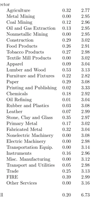
3.1 Disaggregation LevelThe empirical analysis of the model is based on a highly disaggregated partition of the U.S.
Classi…cation (SIC) and are listed in Table 1, along with the Major Group categories that they
include. Agriculture includes the production of crops and livestock, agriculture-related services,
and forestry. Construction includes building and heavy construction and special trade
contrac-tors. The four mining sectors are Major Groups 10 and 12 to 14. The twenty manufacturing
sectors are Major Groups 20 to 39. Transport and utilities includes all forms of passenger and
freight transportation, communications, and electric, gas and sanitary services. Trade includes
both wholesale and retail trade. FIRE is …nance, insurance and real estate. Finally, other services includes personal, business, recreation, repair, health, legal, educational and social services as well as lodging. At this level of disaggregation, agriculture, mining and construction all include some service industries. For example, oil and gas extraction includes drilling and exploration services.
The level of disaggregation is driven by two considerations, namely data availability and com-putational costs. The Bureau of Labor Statistics (BLS) produces sectoral data at discrete levels of disaggregation (divisions, major groups, industry groups and industries). Using a higher disaggre-gation level (say, industry groups) would involve a nontrivial increase in computational complexity because …nding the steady state allocations and prices requires solving a system of 3J + 1 nonlinear
equations, where J is the number of sectors. Also, Dale Jorgenson’s data on sectoral input
ex-penditures, which we use to estimate the parameters of the sectoral production functions, are only available for major groups of the SIC. As we will see below, the level of disaggregation used here allows us to paint a fairly rich portrait of both the macro and microeconomic e¤ects of monetary policy.
3.2 Estimation Strategy
The estimation of this model is computationally demanding for two reasons. First, the number
of structural parameters is very large and, second, the steady state and solution of the model need to be calculated in every iteration of the optimization algorithm. As noted above, …nding the steady state requires solving a large system of nonlinear equations. We respond to this challenge by exploiting the properties of the model and various data to estimate or calibrate the parameters that determine the steady state. Then, with those parameter values …xed, we estimate the parameters that drive the model dynamics using the Simulated Method of Moments (SMM).
The discount rate ( ) is set to 0:997; which is the sample average of the inverse of the gross
ex-post real interest rate for the period 1959Q2 to 2002Q4. The depreciation rate is set to = 0:02:7
The elasticity of substitution between goods produced in the same sector ( ) is set to 8. This value
7In preliminary work, we considered using the sector-speci…c depreciation rates computed by Jorgenson and
Fraumeni (1987) and which very between 0.01 and 0.04. However, results are basically the same as those reported here.
is in the middle of the range used in the literature, and implies an average markup over marginal cost
of approximately 15 percent.8 The parameter that determines the elasticity of substitution between
hours worked in di¤erent sectors is set to 1, following the empirical work by Horvath (2000).9 The
consumption weights j are the average expenditure shares in NIPA from 1959 to 1995 and were
taken from Horvath (2000, p. 87). These weights are listed in the second column of Table 1.10 The
input weights ij and ij are equal to the share of sector i in the materials and investment input
expenditures by sector j; respectively. These shares are computed using data from the 1992 U.S.
Input-Output (I-O) accounts.11 More precisely, the
ijs are computed using the Use Table, which
contains the value of each input used by each U.S. industry, while the ijs are computed using
the Capital Flow Table, which reports the purchases of new structures, equipment and software
allocated by using industry.12 By construction, ij; ij 2 [0; 1] and
J P i=1 ij = J P i=1 ij = 1 for all j:
3.3 Estimation of Production Function Parameters
The production function parameters were estimated using the yearly data on nominal expenditures on capital, labor and materials inputs by each sector collected by Dale Jorgenson for the period
1958 to 1996.13 The nominal expenditures predicted by the model may be obtained from the
8For example, Ireland (2001) sets to 6 while Barsky, House and Kimball (2007) set it to 11. Sensitivity analysis
indicates that our results are robust to using other values employed in the literature.
9Horvath estimates & from an Ordinary Least Square regression of the change in the relative labor supply on the
change in the relative labor share using sectoral U.S. data and …nds & = 0:9996 with a standard error of 0:0027:
1 0Our sector de…nitions di¤er from Horvath’s in that we respectively combine into one sector: agricultural products
and agricultural services; motor vehicles and transportation equipment; and transportation services, communications, electric and gas utilities, and water and sanitary services. The weights in Table 1 have been aggregated accordingly.
1 1I-O tables do evolve over time, for example as a result of technological innovation, but the change is relatively
moderate at the level of disaggregation used here. We carried out a small number of sensitivity experiments and found our results to be robust to small perturbations around the values used.
1 2
We equate commodities with sectors as in the theoretical model where goods of type j are produced only by sector j. This assumption means that we implicitly treat the Make Table of the I-O accounts as diagonal and allows us to estimate the weights using the Use Table alone. The Make Table reports the value of each commodity produced by each domestic industry and, in practice, is not perfectly diagonal. The reason is that the I-O accounts assign a small number of commodities to a Major Group di¤erent from the one where they are produced. For example, printed advertisement is treated as a business service (SIC 73) despite the fact that it is actually produced by printing and publishing (SIC 27). In order to quantify the importance of the o¤-diagonal elements of the Make Table, we computed the share of each commodity type that is produced in each sector. Since the diagonal elements vary between 0.89 and 1, we conclude that the original assumption that associates each commodity type with only one sector is a reasonable approximation for the U.S. economy at this level of disaggregation.
1 3Jorgenson records separately expenditures on materials and energy inputs. In order to be consistent with the
model, where energy is indistinguishable from other materials inputs, we add these two series into a single expenditure category. The complete data set is available at http://post.economics.harvard.edu/ faculty/jorgenson/data and is described in Jorgenson and Stiroh (2000).
…rst-order conditions of the …rm’s problem j j tPtytj = w j tn j t; (31) j j tPtytj = J X i=1 pithji;t; (32) j j tPtytj = t 1 t j t 1 (1 ) j t Ptkjt + QX j t k j t @ t @ktj ! ; (33)
where jt and jt are, respectively, the real marginal cost and the real shadow price of capital in
sector j. Since, in equilibrium, …rms in the same sector are identical, the …rm superscripts are
dropped. The right-hand sides of these equations are, respectively, the wage bill, total
expen-ditures on materials inputs, and the opportunity cost (net of capital gains) of the capital stock plus net adjustment costs. Jorgenson’s data are empirical counterparts of these expressions, but the mapping for capital is imperfect because the data do not include adjustment costs and take into account distortionary taxes, from which our model abstracts (see Jorgenson and Stiroh, 2000,
Appendix B). Although the data set does not contain observations on jtPtytj; it is possible to
construct estimates of j; j; and j as follows. Use two of the three ratios: (31)/(32), (31)/(33)
and (32)/(33), and the condition j + j + j = 1 to obtain a system of three equations with
three unknowns.14 The unique solution of this system delivers an observation of the production
function parameters for a given year. Our estimates of j; j and j are the sample averages of
these yearly observations and their standard deviations are p 2=T where 2 is the variance of the
yearly observations and T = 39 is the sample size.15
Estimates of the production function parameters are reported in Table 2. These estimates
indicate substantial heterogeneity in capital, labor and materials intensities across sectors. Services sectors, especially trade, tend to be labor intensive but so are also construction, coal mining and
some manufacturing sectors like instruments, and printing and publishing. Mining sectors are
generally the most capital intensive of the economy, while construction is the least capital intensive. Material intensity tends to be relatively low in services and mining compared with manufacturing, construction and agriculture. Some manufacturing sectors like oil re…ning, food products, textile
mill products, and lumber and wood are extremely intensive in materials. This heterogeneity in
1 4Given any two ratios, the third one is redundant and may be trivially derived from the other two. Hence,
estimates of the production function parameters are independent of the particular pair of ratios employed.
1 5
In deriving equation (33) from the …rst-order condition for kjt+1, we used the assumption of rational expectations.
Hence, this equation holds up to a mean-zero forecast error. This adds extra noise to the yearly estimates of all production function parameters. However, since the variance of this forecasts error is likely to be small compared with that of the other terms, and since we average over yearly estimates, it is reasonable to assume that the e¤ect of this error on point estimates is small.
production function parameters is statistically signi…cant in that tests of the null hypothesis that
j; j and j are equal in all sectors are strongly rejected by the data.
3.4 Simulated Method of Moments
The remaining parameters are estimated by the Simulated Method of Moments (SMM) using sectoral and aggregate U.S. time series at the quarterly frequency for the period 1964Q1 to 2002Q4. The use of Simulated Method of Moments (SMM) for the estimation of DSGE models was proposed by Lee and Ingram (1991) and Du¢ e and Singleton (1993). Previous applications include Klein and Jonsson (1996), Coenen and Levin (2004) and Coenen and Wieland (2005) for linear models, and Kim and Ruge-Murcia (2007) for nonlinear models. Ruge-Murcia (2007) uses Monte-Carlo analysis to compare various methods used in the estimation of DSGE models and …nds that moment-based estimators are less a¤ected by the stochastic singularity of DSGE models and are generally more
robust to misspeci…cation than Maximum Likelihood.16 The sample starts in 1964 because data
on wages in the service sector are available only after this date, and ends in 2002 because thereafter the BLS stopped reporting sectoral data under the SIC codes.
The sectoral data consist of quarterly series of real wages and PPI (Producer Price Index)
in‡ation rates, computed using raw data taken from the BLS web site (www.bls.gov ).
Unfortu-nately, these data are not available for all thirty sectors in our model. We use sectoral wages for construction, all manufacturing sectors (except electric machinery and instruments for which the data are not available for the complete sample period) and all services sectors. Sectoral wages are constructed by dividing the monthly observations of average weekly earning of production workers by the CPI and averaging over the three months of each quarter.
We use sectoral in‡ation for the fourteen sectors listed in Table 3 for which it is possible to match commodity-based PPIs with their respective sector. Matching commodity-based PPIs with sectors allows us to address the fact that the BLS only started to construct industry-level PPIs
in the mid-1980s. We assess the quality of the match by computing the correlation between the
in‡ation rates constructed using commodity-based and industry-level PPIs for the periods where both index types are available. These correlations are reported in Table 3 and vary between 0.59
for oil and natural gas to almost 1 for tobacco products.17 Notice that although the data set on
1 6
In this application, the length of the simulated series relative to the sample size is 20 and the weighting matrix is the inverse of the matrix with the long-run variance of the moments along the main diagonal and zeros in the o¤-diagonal elements. The latter is computed using the Newey-West estimator with a Barlett kernel and Newey-West …xed bandwidth, that is, the integer of 4(T =100)2=9 where T is the sample size, but results are reasonably robust to using other bandwidths. For the model simulation, innovations are drawn from normal distributions.
1 7
We were unable to compute this correlation for agriculture because no industry-level PPI is available. In preliminary work, we considered using the commodity-based PPI for metals but the correlation with its industry-level equivalent was only 0.148.
sectoral prices and wages is incomplete, sector speci…c parameters will be identi…ed by our structural estimation approach because these parameters also a¤ect observable aggregate and other sectoral
variables through general equilibrium e¤ects. Since the raw data are seasonally unadjusted, we
control for seasonal e¤ects by regressing each series on seasonal dummies and purging the seasonal components.
The aggregate data consist of the quarterly series of the rate of in‡ation, the rate of nominal money growth, the nominal interest rate, per-capita real money balances, per-capita investment and per-capita consumption. With the exceptions noted below, the raw data were taken from the Federal Reserve Economic Database (FRED) available from the Federal Reserve Bank of St-Louis web site (www.stls.frb.org). The in‡ation rate is the percentage change in the CPI. The rate of
nominal money growth is the percentage change in M2. The nominal interest rate is the
three-month treasury bill rate. Real money balances are computed as the ratio of M2 per capita to
the CPI. Real investment and consumption are measured, respectively, by gross private domestic investment and personal consumption expenditures per capita divided by the CPI. The raw invest-ment and consumption series were taken from NIPA. These data are available from the BEA web site (www.bea.gov ). Real balances, investment and consumption are computed in per-capita terms in order to make the data compatible with the model, where there is no population growth. The population series corresponds to the quarterly average of the mid-month U.S. population estimated by the BEA. Except for the nominal interest rate, all data are seasonally adjusted at the source. Since the variables in the model are expressed in percentage deviations from the steady state, all series were logged and quadratically detrended.
In summary, the moments used to estimate the model are the variances and …rst-order autoco-variances of the following 43 series: per-capita consumption, investment and real money balances; the rates of money growth, nominal interest, and CPI in‡ation; the rates of PPI in‡ation in agri-culture, coal mining, oil and gas extraction, nonmetallic mining, food products, tobacco products, lumber and wood, furniture and …xtures, paper, chemicals, oil re…ning, rubber and plastics, leather, and stone, clay and glass; and the real wages in construction, all twenty manufacturing sectors
(ex-cept for electric machinery and for instruments) and all four service sectors. These 86 moments
are used to identify 47 structural parameters. The parameters are 30 sectoral price rigidities, the capital adjustment cost parameter, and the autocorrelation and standard deviation of the produc-tivity, money demand, labor supply and monetary policy shocks. Estimating both parameters of the productivity-shock processes for all sectors would mean estimating 60 parameters. Hence, in order to economize degrees of freedom and sharpen identi…cation, we limit shock heterogeneity to the Division level of the SIC. Thus, we assume one distribution each for agriculture (Division A),
all mining sectors (Division B), construction (Division C), all manufacturing sectors (Division D), and all services sectors (Divisions E through I). This means that we estimate the parameters of …ve rather than of thirty shock distributions. Since draws are independent, however, shock realizations will be di¤erent in di¤erent sectors, whether they are in the same Division or not.
4.
Parameter Estimates and Micro Implications
In this section, we report SMM estimates of the structural parameters of the multi-sector model and examine the microeconomic implications of the model. In particular, we compare our estimates of sectoral price rigidity and the realized price adjustment costs with those based on micro data. We also report SMM estimates for a version of the model where price rigidity is the same in all sectors.
4.1 Sectoral Price Rigidity
SMM estimates of the price rigidity parameters are reported in Table 4. The magnitude of this
parameter varies greatly across sectors and the null hypothesis that its true value is the same for all sectors is strongly rejected by the data (p-value < 0:0001). Hence, heterogeneity in price rigidity is quantitatively important and statistically signi…cant.
The null hypothesis that prices are ‡exible (that is, = 0) cannot be rejected at the 5 percent
level for 17 out of 30 sectors in our sample. Thus, at this level of disaggregation, the majority
of sectors in the U.S. economy are ‡exible price sectors. This point is illustrated in a simple
but revealing way in Figure 1, which plots the distribution of price rigidity parameters.18 This
distribution is highly positively skewed and has a median of only 4.80. Flexible price sectors include producers of primary goods (agriculture and mining), manufactured commodities (for example, tobacco, chemical and petroleum products) and some durable goods (for example, electric and nonelectric machinery, and instruments).
The null of price ‡exibility can be rejected for 13 sectors and the magnitude of is especially
large in eight sectors, namely trade, transport and utilities, primary metal, construction, food, apparel, furniture, and leather goods. Importantly, the …rst two sectors (trade, and transport and utilities) are services, and account respectively for 25 and 21 percent of the Consumer Price Index
in the model economy. These results suggest that price rigidity in the U.S. economy is mostly
concentrated in services.
1 8In related work, Carvalho and Dam (2008) construct a cross-sectional distribution of price stickiness using
ag-gregate U.S. data alone. Their approach is complementary to ours and is based on the observation that di¤erent sectors may be relatively more important than others in determining the response of aggregate variables to shocks at di¤erent frequencies.
In what follows, we quantitatively compare our macro estimates of sectoral price rigidity with estimates computed by Bils and Klenow (2004) and Nakamura and Steinsson (2008a) using U.S.
micro data. One di¢ culty, however, is that micro-based estimates of price rigidity are usually
reported in terms of frequency of adjustments (from which durations may be computed) but our quadratic cost model expresses price rigidity in terms of the size of, rather than the time interval
between, price adjustments. In order to derive the duration spells implied by our rigidity
esti-mates, we exploit the observational equivalence between the Phillips curves in the (log-linearized) quadratic-cost and Calvo models. To see this equivalence, note that the sectoral Phillips curve for a generic sector j in our model is
Et^jt+1=
1
^jt j1 ^jt ˆpjt ;
where pjt = pjt=Pt is the real price and the circum‡ex denotes deviation from steady state. On
the other hand, the sectoral Phillips curve that would be obtained in a version of the model where …rms follow Calvo pricing is
Et^jt+1= 1 ^jt 1 % j (1 %j) %j ^ j t ˆp j t ;
where %j is the probability of not changing prices. The two curves are isomorphic and, given
nu-merical values of the elasticity of substitution ( ) and the discount rate ( ), imply a correspondence
between the rigidity parameter j in the quadratic cost function and the Calvo probability, %j: In
particular, given a value of j > 0, the sectoral Calvo probability is the smaller root that solves19
1
j =
1 %j (1 %j )
%j :
Since under Calvo pricing, signals are independent across …rms and time, the expected price
du-ration is 1=(1 %j). Notice that, by construction, the expected duration cannot be shorter than
one period, which is a quarter in our model. The Calvo probabilities and durations implied by
our estimates of j are reported in Table 4. Since these variables are monotonic transformations
of the js, their distributions share the positive skewness observed in Figure 1.
Durations constructed from the micro-based estimates are also reported in Table 4. The mean durations for producer prices were computed as the inverse of the monthly frequencies of price
1 9
This is a quadratic equation with roots
( 1) + j(1 + ) q
(1 ) j(1 + ) 2 4 j 2
2 j :
Since (1 ) j(1 + ) 2
4 j 2 > 0and ( 1) + j(1 + ) > 0;it follows that both roots are real and
changes for Major Industries reported by Nakamura and Steinsson (see their Table 7), divided by 3
to express them in quarters.20 The mean durations of consumer prices were estimated as follows.
First, each Entry Level Item (ELI) category in the micro data was manually matched into one of our sector de…nitions. Then, sectoral price durations were computed as the weighted average of the durations of ELIs in that sector. The raw ELI durations are those reported by Bils and Klenow (2004) and Nakamura and Steinsson (2008a), and the weights are proportional to those given to
each ELI in the CPI.21 In total, we constructed four sets of micro estimates respectively based on
PPI prices, regular CPI prices and …nal CPI prices from Nakamura and Steinsson, and …nal CPI prices from Bils and Klenow. Final CPI prices include the e¤ect of sales.
A graphic comparison between the durations implied by the estimated DSGE model and those computed from micro data is reported in Figure 2. Along the continuos 45 degree line estimates would match perfectly. Observations marked with a “plus” (“circle”) are macro-based durations for which the null hypothesis that their true value equals the micro-based estimate cannot (can) be rejected at the 5 percent signi…cance level. Although there are outliers in all panels, this …gure
shows that both sets of estimates are in broad quantitative agreement. Furthermore, the …gure
has many more “pluses” than “circles,” meaning that micro and macro estimates are statistically
the same for most sectors. This result is remarkable given the large methodological di¤erences
between the two approaches.
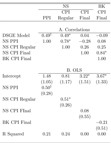
Notice in Figure 2 that macro estimates are better correlated with micro estimates based on
PPI and regular CPI prices than with those based on …nal CPI prices that include sales. This
observation is statistically con…rmed in Table 5, where we report the correlation matrix of all duration estimates (Panel A) and results from Ordinary Least Square (OLS) projections of macro estimates on micro ones and an intercept term (Panel B). The correlation between macro estimates and micro estimates based on PPI prices is 0.49. When one excludes rubber, which is a gross outlier, this correlation increases to 0.65 and is statistically di¤erent from zero. The correlation between macro estimates and estimates based regular CPI prices is 0.49 and statistically di¤erent from zero. Regression results show that in both cases the slope is positive and statistically di¤erent from
2 0Nakamura and Steinsson use di¤erent sector de…nitions from ours, so we match the sectors closest in nature.
However, they respectively combine primary and fabricated metal, and electric and nonelectric machinery into single categories. Given the ambiguity in matching these sectors, we have dropped them from Table 4.
2 1
There were some ELIs for which there was no obvious sectoral match and, consequently, were excluded from the analysis. These were 8 out of 272 ELIs in Nakamura and Steinsson, and 26 out of 350 in Bils and Klenow. Another issue is that the number of ELIs per sector varies considerably. For example, in Bils and Klenow’s data, there are 79 ELIs corresponding to food products, but only 2 corresponding to fabricated metal. This means that not all sectoral mean durations are equally accurate. In order the limit the e¤ect of estimates based on too few ELIs, we restricted the analysis to estimates constructed using at least …ve ELIs. The only exception is tobacco products where cigarettes and cigars account for most of the sectoral output.
zero (although only at the ten percent level for PPI prices), while the intercept is not statistically di¤erent from zero.
In contrast, the correlation between macro estimates and …nal CPI prices, which include sales,
is very close to zero and OLS results show a statistically insigni…cant slope coe¢ cient. These
results are not surprising since our model and data abstract from transitory sales. Moreover,
these results are consistent with what we observe when we compare micro-based estimates among themselves. The correlation between durations based on PPI and regular CPI prices is high (0.78)
and statistically di¤erent from zero,22 but the correlation between either of them and durations
based on …nal prices is low and not statistically di¤erent from zero.23
4.2 Price Adjustment Costs
We now compute estimates of realized price adjustment costs and compare them with those based on micro data and predicted by other sticky-price models. From the de…nition of dividends in Equation
(13), note that the ratio of price adjustment costs to sectoral revenue in our model is simply jt:
By construction, this term is zero in steady state, but an estimate of its average magnitude outside steady state may be computed by means of stochastic simulation. The simulated sample has 1600 observations with innovations drawn from normal distributions but, in order to limit the e¤ect of the initial observation, estimates are computed using only the last 1500 observations. Estimates are reported in Table 6, where we observe that adjustment costs as percent of sectoral revenue range from approximately 0 in, for example, nonelectric machinery to 0.53 in lumber and wood.
The correlation between realized price adjustment costs and the price rigidity estimates reported
in the previous section is basically zero (0.04). The reason is that realizations of jt depend not
only on the structural parameter j; but also on the size of the price change, pljt =pljt 1; which is
optimally chosen by …rms. Thus, for example, realized adjustment costs are somewhat larger in
the paper sector (which has an essentially ‡exible price) than in furniture and …xtures (which has a price duration of …ve quarters) because price changes are typically larger in the former than in the latter (the median price changes are 1.2 and 0.8 percent, respectively). This means that direct micro estimates of price adjustment costs incurred by …rms may not be informative about the structural parameters driving such estimates. One may observe a small ratio of price adjustment costs to revenue precisely because changing prices is so costly, or a large ratio because changing
2 2
This estimate is similar to the correlation of 0.83 between the frequency of price changes for producer prices and regular consumer prices reported by Nakamura and Steinsson (2008a, p. 19) and computed using 153 goods categories.
2 3
Nakamura and Steinsson (2008a) …nd that sales exhibit di¤erent empirical features from regular price changes and so, for example, Kehoe and Midrigan (2007) assume that one-period price discounts involve a smaller menu cost than regular price changes.
prices is a relatively cheap margin for the …rm.
Our estimates of realized price adjustment costs are of similar magnitude to those computed by Nakamura and Steinsson (2008b) for the menu-cost and Calvo-plus models (which vary between 0.004 and 0.72, and between 0.007 and 2.70, respectively), but they are smaller than micro-based estimates by Levy, Bergen, Dutta and Venable (1997), and by Zbaracki, Ritson, Levy, Dutta and Bergen (2004) who …nd that the cost of changing prices in, respectively, a supermarket and a manufacturing …rm are 0.7 and 1.2 percent of revenue. Regarding the former, our estimate for the trade sector (which includes both wholesale and retail trade) is only 0.25 percent of revenue.
4.3 The Kurtosis of Price Changes
Since …rms in the same sector choose the same adjustment size in a given period, the time series of
percental price changes is just the sectoral in‡ation rate. Furthermore, because the propagation
mechanism is linear and shocks are normally distributed, sectoral in‡ation rates are normally distributed as well, and kurtoses are, therefore, close to 3 (see the second column in Table 6). On the other hand, the distribution of the complete sample of price changes is a mixture of the thirty sectoral distributions. This mixture features fat tails and a kurtosis equal to 6.7, which is quantitatively similar to the estimates of 5.4 and 8.5 reported by Midrigan (2008) for non-sale price changes in the AC Nielsen and Dominick’s data sets, respectively.
4.4 Other Parameter Estimates
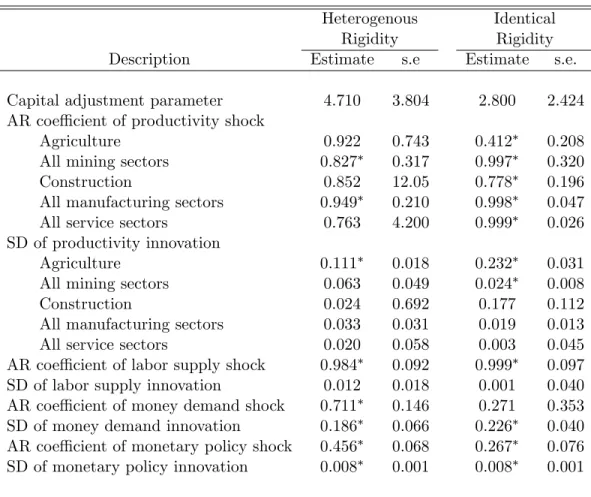
Table 7 reports SMM estimates of the other structural parameters. The estimate of the capital
adjustment cost parameter is 4.71 (3.80), where the term in parenthesis is the standard error. This estimate is not statistically di¤erent from zero and is quantitatively smaller than values reported
in previous literature that estimates using aggregate data alone (see, for example, Kim, 2000,
and Bouakez, Cardia and Ruge-Murcia, 2005). On the other hand, our estimate is in line with
those reported by Hall (2004) and Cooper and Haltiwanger (2006), which are respectively based on industry- and plant-level data and which imply relatively small capital adjustment costs. In our model, input-output interactions induce strategic complementarity in pricing across sectors and greatly amplify the e¤ects of monetary shocks, thereby reducing the quantitative importance of
other real rigidities, like capital adjustment costs.24
Labor supply and money demand shocks are relatively persistent and feature volatile innova-tions, while monetary policy shocks are only mildly persistent and not very volatile. In particular,
2 4
For analytical results illustrating this ampli…cation mechanism in the context of roundabout models like ours, see Basu (1995).
the estimated autoregressive coe¢ cient is 0.46 (0.07), which is smaller than, but still consistent with, the estimate that would be obtained from an unrestricted …rst-order autoregression of the
rate of growth of money supply, which is 0.58 (0.09).25
The autoregressive coe¢ cient of productivity shocks varies from 0.83 in mining to 0.95 in man-ufacturing, but the null hypothesis that these values are the same in all sectors cannot be rejected at the 5 percent level. In contrast, there is substantial heterogeneity in the standard deviation of productivity innovations across sectors. Estimates range from 0.02 in services to 0.11 in agriculture and the null hypothesis that standard deviations are the same in all sectors can be rejected at the 5 percent level. In general, productivity innovations in primary sectors (agriculture and mining) are substantially more volatile than in other sectors.
Our results are similar to those in Horvath (2000), who also …nds innovations to agriculture and mining to be the most volatile. Horvath estimates the parameters of neutral sectoral productivity shocks from the residuals of outputs minus weighted factor inputs using energy usage to correct for variations in capital utilization. In order to compare the two sets of estimates, notice that the
standard deviation of the innovation of Horvath’s neutral shock in sector j correspond to j zj in
our model with labor-augmenting shocks. Figure 3 plots the two sets of estimates, with a “plus” (“circle”) denoting cases where the null hypothesis that the true value equals the one estimated
by Horvath cannot (can) be rejected at the 5 percent signi…cance level. The hypothesis cannot
be rejected for 25 of the 30 sectors in our sample but is rejected for oil and gas extraction, paper, leather, metal mining, and tobacco products. In the latter two cases, the hypothesis would not be rejected at the 1 percent level. Finally, the correlation between both sets of estimates is 0.41 and statistically di¤erent from zero.
Overall, results reported so far support the idea that our highly disaggregated DSGE model with heterogenous price rigidity captures reasonably well basic features of the micro data, and motivate the policy analysis carried below in Sections 5 through 7.
4.5 Model with Identical Price Rigidity Across Sectors
In this section, we report parameter estimates for a restricted version of the model where price
rigidity is the same in all sectors (that is, j = for all j). Although this restriction is rejected
by the data, this model constitutes a useful benchmark to study the contribution of heterogeneity in price rigidity to the propagation of monetary policy shocks.
The estimate of the price rigidity parameter is = 6.48 (0.92), which implies a duration of
1.58 quarters for prices in all sectors (see Panel B in Table 4). Recall that the median rigidity
parameter in the heterogeneous model is 4.80, which implies a duration of 1.48 quarters. Both duration estimates (that is, 1.58 and 1.48) are in the ranges of median price durations reported in micro-based studies. For example, the median price duration varies between 1.4 and 1.8 quarters in Bils and Klenow (2004), between 1.2 and 2.4 in Klenow and Kryvtsov (2008), and between 1.4 to 3.6 quarters in Nakamura and Steinsson (2008a).
In turn, all of these estimates are generally smaller than those obtained using aggregate data alone. See, for example, Gali and Gertler (1999), Smets and Wouters (2003), Christiano, Eichen-baum and Evans, (2005), and Bouakez, Cardia and Ruge-Murcia (2005), who respectively report “aggregate” price durations of 5.9, 10.5, 2.5 and 6.5 quarters. Large price rigidity estimates sub-stantially contribute to the empirical success of (one-sector) sticky-price DSGE models but they are now considered implausible in light of the recent evidence on price rigidity at the micro level. As we will see below, our heterogenous, multi-sector DSGE model can reconcile fully-speci…ed macro models with the micro data.
Table 7 reports estimates of the other parameters of the restricted model. They are
gener-ally consistent with those obtained for the heterogenous model though, as one would expect, the parameters of the sectoral productivity shocks are more precisely estimated.
5.
Sectoral E¤ects of Monetary Policy Shocks
In this Section, we study the e¤ects of a monetary policy shock on sectoral outputs and in‡ation
rates and on relative prices. More precisely, we consider the e¤ects of an innovation that
unex-pectedly increases the rate of money growth by 1 percent. Thereafter, with innovations set to zero,
money growth gradually returns to its steady state at the rate : We plot the responses associated
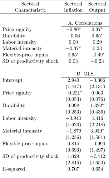
with this shock, and examine the relation between the initial sectoral response and several sectoral characteristics using unconditional correlation coe¢ cients and OLS regressions.
The sectoral characteristics are price rigidity (measured by the implied durations reported in
Table 4), whether the sector produces a durable good or not,26 labor and materials intensity,27 the
standard deviation of the productivity shock, and the proportion of materials that are purchased
from ‡exible-price producers. For the computation of the latter variable, we classify as
‡exible-price producers all sectors for which the null hypothesis that j = 0 cannot be rejected (see Table
4). Then, for each sector in our sample, we add up the input shares (from the Use Table) of
2 6
This classi…cation is made following the BLS de…nition of durability. The durable-good sectors are construction, lumber and wood, furniture and …xtures, primary metal, fabricated metal, nonelectric machinery, electric machinery, transportation equipment, instruments, miscellaneous manufacturing, and stone, clay and glass.
2 7Since production functions exhibit constant returns to scale, intensities are linearly dependent. For this reason
those ‡exible-price sectors. The average sector buys around 60 percent of its materials inputs from ‡exible-price sectors, but the proportion varies greatly across sectors, ranging from 18 percent in apparel to 88 percent in tobacco products.
5.1 In‡ation
The responses of sectoral in‡ation rates are plotted as continuos lines in Figure 4. This …gure shows that all in‡ation rates increase following the shock but that there is substantial heterogeneity in
the size and dynamics of the sectoral responses. Some sectoral in‡ations react strongly to the
shock but return rapidly to their steady state, while others respond weakly and return slowly and monotonically to their steady state.
The correlation between the magnitude of the initial response of in‡ation and sectoral charac-teristics, and the results of an OLS projection of the former on the latter and a constant term, are respectively reported in Panels A and B of Table 8. The correlation between the in‡ation response and price rigidity is negative, quantitatively large ( 0:8) and statistically signi…cant. Thus, as one would expect, sectors with ‡exible prices (that is, shorter price durations) tend to increase their prices by more than sectors with rigid prices, following an expansionary monetary policy shock.
The correlation with the proportion of materials purchased from ‡exible-price producers is
positive and signi…cant. This result re‡ects the fact that marginal costs tend to rise by more in
sectors whose intermediate inputs have ‡exible prices. The correlation with materials intensity
is negative, although only marginally signi…cant. Thus, sectors that require more materials as
productive inputs tend to increase their prices by less after a monetary shock. This mechanism is emphasized by, for example, Basu (1995). However, the latter two correlations are not signi…cant
once we control for other factors. In particular, the OLS results in Panel B show that the price
rigidity coe¢ cient is statistically signi…cant at the 5 percent level whereas the other coe¢ cients
are not.28 On the basis of this analysis, we conclude that heterogeneity in price rigidity is the
most relevant factor to understand the cross-sectional heterogeneity in sectoral in‡ation responses to monetary policy shocks.
5.2 Relative Price Dispersion
Since the equilibrium is symmetric within sectors but asymmetric across sectors, sectoral relative
prices are not all equal to 1. To avoid ambiguity, we focus on the relative price pjt = pjt=Pt; which
is also the real price. The distribution of relative prices (not shown) has a mean of 0.90 and a
2 8
We computed the correlation matrix of the regressors and found that they range from 0:63to 0:34: Thus, it is unlikely that these results are driven by collinearity among the explanatory variables.
relatively large standard deviation of 0.28. Since sectoral in‡ations react di¤erently to a monetary policy shock, it follows that monetary policy shocks induce changes in the distribution of relative prices. This can be seen in Figure 5 which plots the standard deviation of relative prices following the monetary shock under the heterogenous price rigidity model (see the continuos line). Notice that starting at the steady state value of 0.28, the standard deviation rises to 0.86 in the quarter following the shock. Hence, there is a large increase in relative price dispersion as a result of the monetary policy shock. This result is primarily due to the strong price response by ‡exible price
producers. Moreover, the e¤ects of monetary policy on relative prices dispersion are long-lived
and only after six quarters does the standard deviation approaches the initial one.
In contrast, under the model with identical price rigidity across sectors (see the dotted line), the e¤ect of the monetary policy shock on relative price dispersion is muted and the standard deviation is almost unchanged after the shock.
5.3 Output
We now consider the e¤ects of a monetary policy shock on sectoral outputs. The continuos
lines in Figure 6 show that sectoral outputs increase following the monetary policy shock. The
only exception is tobacco products whose output initially contracts by 0.07 percent but eventually expands after the third quarter. Thus, in general, there is positive output comovement following a monetary shock.
This result contrasts with the prediction of previous two-sector models (see, for example, Ohanian, Stockman and Kilian, 1995, and Barsky, House and Kimball, 2007) where the output of the ‡exible-price sector contracts, while that of the rigid-price sector expands, after an
expan-sionary monetary policy shock. In a striking example in Barsky, House and Kimball, aggregate
output stays unchanged and money is neutral at the aggregate level despite the fact that some
prices are sticky. The negative output comovement arises primarily from the absence of
input-output interactions. The increase in the price of ‡exible- relative to rigid-price goods leads to a
strong substitution e¤ect on the part of households and, therefore, to opposite output e¤ects of
monetary policy. As we saw above, in our model, monetary policy shocks also produce changes
in relative prices as a result of heterogeneity in price rigidity, but the substitution e¤ect does not drive the output dynamics because …rms require the output of other …rms to produce their own good. The positive output comovement implied by our multi-sector model is consistent with the empirical evidence reported by Barth and Ramey (2001), Dedola and Lippi (2003) and Peersman and Smets (2005).
the least are producers of primary goods (agriculture, metal mining, oil and gas extraction) or
basic manufactured commodities (tobacco production and chemicals). The sector that responds
the most is construction, followed by lumber and wood, primary metal, transportation equipment, stone, clay and glass, and fabricated metal. Notice that all these sectors are producers of durable goods and that the latter ones are large inputs to construction: the fraction of materials input expenditures by construction that go into lumber and wood, primary metal, and stone, clay and glass, and fabricated metal are 10.3, 2.8, 8.4, and 12.6 respectively, while the proportion of capital
input expenditures that goes into transportation equipment is 33.4 percent. This observation
suggests that the construction sector plays a prominent role in the transmission of monetary policy through input-output interactions.
The relation between sectoral output responses and sectoral characteristics is reported in Table
8. In Panel A, the correlation between the output response and whether the sector produces a
durable good is positive, quantitatively large (0:65) and statistically signi…cant. Thus, producers of durable goods tend to increase their output by more than nondurable good producers following a monetary policy shock. The correlation with the proportion of inputs from ‡exible-price sectors is negative and statistically signi…cant. The reason is that sectors with a lower proportion of ‡exible-price inputs experience a smaller increase in marginal cost following a monetary policy shock and,
therefore, have a greater scope to increase their output. The correlation with price rigidity is
positive but only marginally signi…cant at the 5 percent level. Thus, as one would expect, sectors
with rigid prices tend to increase their output by more than sectors with ‡exible prices. The
correlation with other variables is not statistically di¤erent from zero.
In Panel B, OLS results indicate that the coe¢ cients of durability and material intensity are statistically signi…cant at the 5 percent level, while the other coe¢ cients, including those of the
proportion of ‡exible-price inputs and price rigidity, are not signi…cant. We conclude that the
most important factor to understand the cross-sectional heterogeneity in sectoral output responses
to monetary policy is whether the sector produces a durable good or not. This result is due to
the input-output structure of our model and, in particular, to the fact that the general increase
in output by all sectors requires an increase in the production of investment goods. Since the
production of investment goods is concentrated in relatively small sectors, their output response is proportionally larger than that of other sectors. The implication that durable-good producers react strongly to monetary policy shocks is consistent with the VAR evidence in Barth and Ramey (2001) and Erceg and Levin (2006).