Université de Montréal
Learning A Graph Made of Boolean Function Nodes: A New Approach in Machine Learning
par
Mouna Mokaddem
Département d’informatique et de recherche opérationnelle Faculté des arts et des sciences
Mémoire présenté à la Faculté des études supérieures en vue de l’obtention du grade de Maître ès sciences (M.Sc.)
en Informatique
August, 2016
c
Université de Montréal Faculté des études supérieures
Ce mémoire intitulé:
Learning A Graph Made of Boolean Function Nodes: A New Approach in Machine Learning
présenté par: Mouna Mokaddem
a été évalué par un jury composé des personnes suivantes: PrénomPrésident NomPrésident, président-rapporteur PrénomDirecteur NomDirecteur, directeur de recherche
RÉSUMÉ
Dans ce document, nous présentons une nouvelle approche en apprentissage machine pour la classification. Le cadre que nous proposons est basé sur des circuits booléens, plus précisément le classifieur produit par notre algorithme a cette forme. L’utilisation des bits et des portes logiques permet à l’algorithme d’apprentissage et au classifieur d’utiliser des opérations vectorielles binaires très efficaces. La qualité du classifieur, pro-duit par notre approche, se compare très favorablement à ceux qui sont propro-duits par des techniques classiques, à la fois en termes d’efficacité et de précision. En outre, notre approche peut être utilisée dans un contexte où la confidentialité est une nécessité, par exemple, nous pouvons classer des données privées. Ceci est possible car le calcul ne peut être effectué que par des circuits booléens et les données chiffrées sont quantifiées en bits. De plus, en supposant que le classifieur a été déjà entraîné, il peut être alors facilement implémenté sur un FPGA car ces circuits sont également basés sur des portes logiques et des opérations binaires. Par conséquent, notre modèle peut être facilement intégré dans des systèmes de classification en temps réel.
Mots clés : Apprentissage machine, classification, classifieur, données privées, FPGA.
ABSTRACT
In this document we present a novel approach in machine learning for classification. The framework we propose is based on boolean circuits, more specifically the classi-fier produced by our algorithm has that form. Using bits and boolean gates enable the learning algorithm and the classifier to use very efficient boolean vector operations. The accuracy of the classifier we obtain with our framework compares very favourably with those produced by conventional techniques, both in terms of efficiency and accuracy. Furthermore, the framework can be used in a context where information privacy is a ne-cessity, for example we can classify private data. This can be done because computation can be performed only through boolean circuits as encrypted data is quantized in bits. Moreover, assuming that the classifier was trained, it can then be easily implemented on FPGAs (i.e., Field-programmable gate array) as those circuits are also based on logic gates and bitwise operations. Therefore, our model can be easily integrated in real-time classification systems.
CONTENTS
RÉSUMÉ . . . iii
ABSTRACT . . . iv
CONTENTS . . . v
LIST OF TABLES . . . viii
LIST OF FIGURES . . . ix LIST OF APPENDICES . . . x LIST OF ABBREVIATIONS . . . xi CHAPITRE 1 : INTRODUCTION . . . 1 CHAPITRE 2 : PRELIMINARIES . . . 3 2.1 Machine Learning . . . 3 2.1.1 Definition . . . 3 2.1.2 Supervised Learning . . . 4 2.1.3 Training-Validation-Testing . . . 5
2.1.4 Model’s complexity, Hyperparameters, Bias-variance tradeoff . 6 2.1.5 Model Selection : randomized search, grid search . . . 7
2.1.6 Regularization . . . 7
2.2 Graphs and Trees . . . 8
2.3 Entropy . . . 8
2.4 Support Vector Machine . . . 10
2.5 Decision Trees . . . 12
2.6 Artificial Neural Networks : Multilayer Perceptron . . . 13
2.7.1 Definition . . . 15
2.7.2 Boosting . . . 15
2.7.3 Bagging . . . 16
2.8 Random Forests . . . 16
CHAPITRE 3 : BOOLEAN CIRCUIT . . . 18
3.1 Circuit . . . 18
3.2 FPGA . . . 21
3.3 Artificial Neural networks and FPGA . . . 23
3.4 Cryptography . . . 25
CHAPITRE 4 : PROPOSED ALGORITHM . . . 28
4.1 Data Preprocessing . . . 28 4.2 Greedy Initialization . . . 29 4.2.1 Maximizing probability . . . 31 4.2.2 Maximizing information . . . 33 4.2.3 Implementation . . . 36 4.3 Leaf optimization . . . 37 4.4 Node optimization . . . 39 4.5 Regularization . . . 41
4.6 Other variants of the algorithm using ensembles of graphs . . . 42
4.6.1 2-stage combination of classifiers . . . 43
4.6.2 Bagging . . . 44
4.7 Connexion with other approaches : Multilayer Perceptron, Random Forest 44 4.7.1 Connexion with Multilayer Perceptron . . . 44
4.7.2 Connexion with Random Forest . . . 45
CHAPITRE 5 : EXPERIMENTAL RESULTS . . . 47
5.1 Methodology . . . 47
CHAPITRE 6 : CONCLUSION . . . 51 BIBLIOGRAPHIE . . . 53
LIST OF TABLES
3.I 2-gate, AND . . . 19
3.II 3-gate, Majority . . . 19
3.III x⊗ y ⊗ z = v for five training examples . . . 21
4.I Example of maximizing probability . . . 32
4.II Truth table of the gate F1 . . . 33
4.III Truth table of the gate F2 . . . 33
4.IV Truth table of the gate F3 . . . 33
4.V Classifier 1 . . . 34
4.VI Classifier 2 . . . 34
4.VII Input data occurrence counts . . . 36
4.VIII Input data counts sorted according to rightmost column (target T = 1) with the best cut . . . 36
5.I Test set classification error on binarized MNIST (0,1,2,3,4 versus 5,6,7,8,9) and CONVEX . . . 48
LIST OF FIGURES
3.1 A depth 3 classifier F made of 7 2-gates for data x = (x1; x2; ...; x10) 20
3.2 FPGA’s architecture . . . 22
4.1 Greedy algorithm . . . 31
4.2 Leaf optimization in a tree . . . 38
4.3 Leaf optimization in a graph . . . 38
4.4 Node’s optimization counting ones . . . 40
LIST OF APPENDICES
LIST OF ABBREVIATIONS
AI Artificial Intelligence ANN Artificial Neural Network CNN Convolutional Neural Network
CPU Central Processing Unit DNA Deoxyribonucleic Acid
DNN Deep Neural Network RF Random Forest
FPGA Field Programmable Gate Array GPU Graphics Processing Unit
ML Machine Learning MLP Multilayer Perceptron SNN Spiking Neural Network SVM Support Vector Machine
CHAPITRE 1
INTRODUCTION
Recently, machine learning classification has been used for several tasks such as me-dical diagnosis, genomics predictions, face recognition and financial predictions. More particularly some machine learning models have shown impressive results on classifica-tion tasks including deep neural networks. However, the digital implementaclassifica-tion of these models is greedy in terms of computations (i.e., floating-point or fixed-point multiplica-tion). In this document, we will introduce a new approach in machine learning classifica-tion that generates a classifier which is based on a boolean circuit. Using bits and boolean gates enables the learning algorithm and classifier to use very efficient boolean vector operations making it suitable for consumer applications on low-power devices. Moreo-ver, in some of the applications mentioned at the beginning of this paragraph, there exist concerns about information privacy. In other terms, it is important that the data remains confidential. And lately, more interest has been drawn, in the scientific community, to the question of how we can apply machine learning classification on encrypted data [1, 3, 10]. Our approach can address perfectly this issue since in such context, compu-tation can be performed only through boolean circuits as encrypted data is quantized in bits. In this project, our main objective is to study the characteristics of a supervised bi-nary classification algorithm that meets the requirements of an environment where data privacy is a necessity. Indeed, the framework we will present is based on boolean circuits, more specifically, the classifier produced by our algorithm has that form. Furthermore, assuming that the classifier was trained, it can then be easily implemented on FPGAs (i.e., Field-programmable gate array) as those circuits are also based on logic gates and bitwise operations. In fact, FPGAs have abundant logic resources (i.e., logic gates), so they can carry out and speed up the computation of our classifier. Moreover, their power efficiency and portability make them ideal for real-time classification systems.
Although our original motivation was unsupervised learning, we have decided to concentrate first on supervised learning in order to study the model’s ability to find a
connection between input and output observations which we believe is much easier than the ability to extract latent variables in the context of unsupervised learning. Once one is acquainted with the framework, a straightforward supervised learning algorithm for binary classification emerges naturally. Studying the properties of this simple algorithm we find its performance surprisingly good, both in terms of efficiency and accuracy. It offers an interesting alternative to neural nets and support vector machines. This is despite the relative maturity of these established techniques, compared with our new framework.
The outline of this document is as follows : in chapter 2, we will set the context of our project by reviewing some basic concepts related to machine learning and some approaches that were compared to ours. Chapter 3 will be for describing the new frame-work we propose then presenting two fields related to the context of our approach which are FPGAs and secure multi-party computation. In chapter 4, we will introduce the algo-rithm describing its three main steps, greedy initialization, leaf’s optimization and node’s optimization followed by a discussion about conceptual similarities and differences with neural nets and random forests. Chapter 5 will be for reporting experimental results and comparison with other approaches’ baselines. Finally, the last chapter will be to conclude and give potential future improvements.
CHAPITRE 2
PRELIMINARIES
In this chapter, we will present some basic concepts related to the context of our project. We will define them formally and for every concept we will discuss points that have been useful either to build our approach or to compare it to other approaches of the literature.
2.1 Machine Learning 2.1.1 Definition
Machine learning is a branch of artificial intelligence that provides computers with the ability to learn autonomously from data. It studies the design of algorithms that learn from input observations, also referred to as examples, instead of relying on hard coded rules. This field, being in the intersection of AI and statics, is about building a model that extracts knowledge from a training set (i.e., the set of examples) in order to make predictions or decisions on unseen examples. The parts of knowledge that a machine learning algorithm tries to capture from data are called patterns and/or features. We will use both words in the rest of the document to express the aforementioned meaning. There are several real-world problems that can be solved using machine learning such as pattern recognition, medical diagnosis, machine translation, self-driving cars, etc. There exists different machine learning scenarios that can be classified according to the types of training data available to the learner, the order and method by which training data is received and the test data used to evaluate the learning algorithm[20]. Instances of those scenarios are supervised learning, unsupervised learning, reinforcement learning, etc. Our approach that will be presented later in the document describes a supervised algorithm, for that reason we will focus on the supervised aspect of machine learning in the following definitions.
2.1.2 Supervised Learning
Supervised learning also known as predictive modelling is the process of making predictions using labelled data. In fact, the supervised learning algorithm is supplied a training dataset D that consists of a set of pairs {zi}ni=1= {(xi, yi)}ni=1 where xi ∈ IRd is
an input object and yi∈ IR the desired output of xi(also known as target) and is required
to find a decision function f that will yield a prediction f (xtesti ) = ˆyi. Hence the task of learning here is to capture the mapping between the inputs and its corresponding outputs in order to make predictions on unseen data later on. In this document, we will consider examples {zi}ni=1∈ D to be independent and identically distributed (i.i.d). When the
tar-get yiis continuous, the process is called regression. When the target yiis discrete, the
learning task consists in a classification. For example f may predict an animal species or a handwritten digit. Our contribution, that will be presented in the following chap-ters, consists of an algorithm for classification based on a new approach. There are two variations of classification depending on the value(s) that the target yi can take : binary
classification is when yi is a binary value whereas multi-category classification when yi
can take three values or more. The performance of f is estimated through a loss function L( f , z) and a dataset D which defines the empirical risk ˆR also known as the expected loss in D ∈ IRd: ˆ R( f , D) = ED[L( f , z)] = 1 n n
∑
i=1 L( f , zi), D = {z1, ..., zn} (2.1)Lcan be of different natures depending on the task to be considered. For classification tasks, L can be chosen to count misclassification error as :
L( f , (x, y)) = 1( f (x)6=y) (2.2)
In which case, ˆR( f , D) will measure the average classification error rate of decision function f over dataset D. So learning means finding the best function ˆf∗ in F that minimizes the empirical risk ˆR on the training set (a regularization term Ω( f ) can be
added, further details for regularization will be given later in the chapter) : ˆ f∗= arg min f∈F J( f ) (2.3) J( f ) = ˆR( f , Dtrain) + Ω( f )
Supervised learning comes in contrast of unsupervised learning that tries to extract struc-ture from unlabelled data.
2.1.3 Training-Validation-Testing
The dataset D used to estimate the risk is finite thus the empirical risk is a biased estimator. In fact, to estimate the real risk a training set that contains an infinite number of examples should be used in order to model perfectly the distribution of D. However practically speaking, this is impossible. Moreover, when minimizing the empirical risk the model is encouraged to perform better on the trained points of the training set than on the other points of the dataset. Therefore, any performance measured on the training set will be most of the time biased (i.e., optimistic). For that reason, the dataset is in practice divided into three subsets : training set Dtrain, validation set Dvalid and test
set Dtest, the last two are generally smaller than the first one. We make sure that the
model will generalize well on examples other than training examples in the following way : f is trained on Dtrain until its error doesn’t further improve on Dvalid (i.e., Dvalid
is used to choose good values of hyperparameters : we will introduce the concept of hyperparameters in the next subsection), finally its performance will be measured over Dtest. Without this division, a model could learn to perform well on D just by stocking
the dataset’s examples and their corresponding targets yet not be able to conserve the same performance for unseen data (i.e., the model is not able to generalize well over examples).
2.1.4 Model’s complexity, Hyperparameters, Bias-variance tradeoff
There are two types of models in machine learning, parametric and non-parametric models. Parametric models are based on a fixed number of parameters θ (scalars, vectors or matrices) to characterize their choice of f in the space of functions F. Therefore, the learning task will consist in optimizing fθ i.e., minimize J( fθ) in order to find the best
parameters. Gradient descent is a good example of an optimization algorithm used to train Artificial Neural Networks. Non parametric memory-based models use the training set for essentially memorizing it directly to model the distribution of D. Kernel SVM is a well-known example of non parametric models [4]. The work presented in this document is a parametric machine learning algorithm that trains by using greedy optimisation and hill climbing.
The number and dimensions of parameters θ define the size of the space of functions F which is referred to as the model’s complexity. There exists a point of optimal com-plexity which corresponds to the lowest value of the generalization error. The number of parameters can greatly influence the quality of the classifier. Variables that are not learned by the algorithm like the number of parameters are called hyperparameters. In fact, they play a role, among other roles, in controlling the model’s complexity. When F is big (i.e., the model’s complexity is high), we have more flexibility to choose the best function ˆf∗ that minimizes the real empirical risk. However, for a high model’s complexity, the learning algorithm will tend to learn too closely Dtrain but poorly
mo-del the true distribution that data comes from, i.e., it will generalize poorly on other samples from that distribution and thus the generated prediction function f will give an empirical error equal or close to zero over Dtrain but a very high one over Dtvalid and
Dtest. This phenomenon is called overfitting. In contrast, reducing too much the model’s complexity will certainly prevent f from overfitting its training set but f won’t be able to model adequately the dataset. Here the problem is referred to as underfitting. A low complexity implies a high bias, a high complexity implies a high variance . Therefore, there should be a tradeoff between the model’s complexity and the generalization over examples, this is called the bias-variance tradeoff. The balance between the bias and
the variance is controlled by hyperparameters (i.e., also controlled by regularization, which will be introduced in the following).
2.1.5 Model Selection : randomized search, grid search
Hyperparameters control a model’s complexity and thus the ability of the model to learn and generalize well. The procedure to select the best values of hyperparameters is referred to as model selection. As aforementioned, the model should be trained on the training set (i.e., Dtrain) to find parameters then tested on the validation set (i.e., Dvalid) to
find values of hyperparameters that minimize the error. Note here that the model should not be tested on the test set (i.e., Dtest) until best values of hyperparameters will be found
on the Dvalid. A solution on how to construct a validation set is to divide the dataset into
two parts of the corresponding proportions : the majority of examples for training set 80% Dtrain and the rest 20% Dvalidwill serve to compare different values of
hyperpara-meters. The values of hyperparameters that give the best performance on the validation set Dvalid are selected and then the selected model will be applied on the test set Dtest to
estimate its expected generalization performance. There are two generic approaches in order to choose the list of values of hyperparameters to be tested : randomized search which samples a given number of candidates from the hyperparameter space according to a specified distribution and grid search which considers all hyperparameter combi-nations on a grid. In fact in grid search, we dress a list of the to be tested values of every hyperparameter of the model then construct the list of every possible combination of those hyperparameters (i.e., constructing a grid of hyperparameters ) that way we will exhaustively consider every combination. In our project, we chose to use grid search fol-lowing our intuition about the values of hyperparameters that should be tested and thus we were able to dress a list of suitable candidates.
2.1.6 Regularization
The complexity of the model f and consequently the risk of overfitting over Dtrain
of regularization are : 1. add a term to the objective function. 2. inject noise. As for the former, it consists in adding to the objective function, during the training, a term that penalizes some parameters of the model under certain conditions. For the latter, an artificial noise is added to the input or/and output samples in the training process which will improve the model’s robustness regarding input inaccuracies to avoid overfitting. Similarly to the "dropout" technique used when training neural networks [27], we will use the second method in our algorithm by artificially injecting noise at all levels during the training step.
2.2 Graphs and Trees
Definition 1. A graph is a representation of a set of objects, called nodes, where some of them are interconnected. The link that connects a pair of nodes is called edge [30]. The edges may be directed or undirected. A degree of a node of a graph is the number of edges incident to the node [5]. In this document we will use directed graphs where the degree of all nodes will be the same (i.e., the degree is equal for all nodes).
Definition 2. A tree is a connected graph with no cycle (i.e., a walk consists of a se-quence of nodes starting and ending at the same node, with each two consecutive nodes in the sequence adjacent to each other in the graph). The edges of a tree are known as branches. Elements of trees are called nodes. The nodes without child nodes are called leaf nodes.
Definition 3. A forest is an acyclic graph. It can be described as the disjoint union of one or more trees.
2.3 Entropy
Definition 4. The entropy of a discrete random variable X with a probability mass func-tion (i.e., pmf) pX(x) is
H(X ) = −
∑
x
The entropy measures the expected uncertainty in X. We also say that H(X) is ap-proximately equal to how much information we learn on average from one instance of the random variable X. Customarily, we use the base 2 for the calculation of entropy.
Consider now two random variables X,Y jointly distributed according to the p.m.f p(x,y). We now define the following two quantities :
Definition 5. The joint entropy is given by
H(X ,Y ) = −
∑
x,y
p(x, y) log p(x, y) (2.5)
The joint entropy measures how much uncertainty there is in the two random va-riables X and Y taken together.
Definition 6. The conditional entropy of X given Y is
H(X |Y ) = −
∑
x,y
p(x, y) log p(x|y) = −IE[log(p(x|y))] (2.6)
The conditional entropy is a measure of how much uncertainty remains about the random variable X when we know the value of Y.
Properties. The entropic quantities defined above have the following properties : • Non negativity : H(X) ≥ 0, entropy is always non-negative. H(X) = 0 iff X is
deterministic.
• Chain rule : We can decompose the joint entropy as follows :
H(X1, X2, ..., Xn) = n
∑
i=1H(Xi|Xi−1) (2.7)
where Xi−1= {X1, X2, ..., Xi−1} For two variables, the chain rule becomes :
H(X ,Y ) = H(X |Y ) + H(Y ) = H(Y |X ) + H(X )
(2.8)
• Monotonicity : Conditioning always reduces entropy :
H(X |Y ) ≤ H(X ) (2.9)
• Maximum entropy : Let χ be set from which the random variable X takes its values, then
H(X ) ≤ log |χ| (2.10)
The above bound is achieved when X is uniformly distributed.
2.4 Support Vector Machine
Support vector machines (SVMs) are supervised learning models associated with learning algorithms that perform, amongst other type of classification, binary linear clas-sification. A binary linear classifier can be visualized as a model that splits a high dimen-sional input space D into two regions C1 and C2 with a hyperplane H referred to as a decision boundary and then classifying a new example xtest ∈ IRd will be according to
its position from H. The hyperplane H is defined by a weight vector w ∈ IRd and a bias b∈ IR which are parameters of the model. The function that tells whether xtest belongs
to one region or another (i.e., C1 or C2) is called discriminative function defined by :
y(x) = wTx+ b =
∑
i
wixi+ b (2.11)
The decision function that predict the category of xtest is :
g(x) = C1, if y(x) > 0 C2, if y(x) < 0 (2.12)
The model we describe requires that D to be linearly separable (i.e., this condition is generally not respected as certain approximations may be done, we will present them below) which is not always the case but we will see later that SVMs could perform a non-linear classification by using what is called the kernel trick. Given a training
data-set of n examples of the form (x1,t1), ..., (xn,tn) where xi ∈ IRd and ti ∈ −1, 1, SVM’s
model aims at finding the maximum-margin hyperplane that divides the group of points xi whose ti = −1 from the group of points whose ti = 1. The margin is defined as the
distance between the hyperplane and the nearest point xifrom either groups. Formally it
is a signed distance given by : tiy(xi) ||w|| =
ti(wTxi+ b)
||w|| , if xiis well-classified then the mar-gin will be positive, else it will be negative. SVM will be about finding the hyperplane that maximizes the margin which is formally expressed by :
arg maxw,b{
1
||w||min[ti(w
Tx
i+ b)]}
To prevent data points from falling into the margin, we add the following constraint : ti(wTxi+ b) ≥ 1
Consequently, min[ti(wTxi+ b)] = 1. Moreover, as mentioned before, some
approxima-tions are done to get around the constraint of linear separability : some terms will be added to the objective function. Those additional terms are referred to as slack variables and express that all predictions have to be within an ε range of the true predictions. We can write the optimization problem of SVM as the following :
arg min w,b,εn 1 2||w|| 2+C n
∑
i=1 εi s.t ti(wTxi+ b) ≥ 1 − εi (2.13) εi≥ 0 f or i= 1, ..., nWe have previously mentioned that there is a way to construct a non-linear classifier for the maximum-margin hyperplane algorithm (i.e., SVM), the kernel trick. "The resulting algorithm is formally similar, except that every dot product is replaced by a non-linear kernel function. This allows the algorithm to fit the maximum-margin hyperplane in a transformed feature space. Although the classifier is a hyperplane in the transformed feature space, it may be nonlinear in the original input space" [32]. In our project, we are using the radial basis function kernel (RBF kernel) which is defined for two examples xi
K(xi, xj) = exp(−
||xi− xj||2
2σ2 ) where ||xi− xj|| the squared euclidean distance the of two
example vectors and σ is a free parameter. The reader interested in kernel method is invited to read [12].
2.5 Decision Trees
In machine learning, decision trees are non-parametric supervised learning methods that use a tree-like graph as a predictive model. They are commonly used for classifica-tion (also can be used for regression) and are referred to as classificaclassifica-tion trees. Decision trees can perform both binary and multiclass classification. Classification trees have a particular structure : leaves represent class labels, nodes represent attributes (i.e. un-learned feature) of input samples and branches represent conjunctions of values that an attribute can take. During training, the tree is learned from top to bottom (i.e., from the root node to the leaves) by splitting the training set into subsets based on an attribute va-lue test. This process is recursive i.e., repeated on each derived subset and stops when the subset at a node has all the same value of the target variable, or when splitting no longer adds value to the predictions. For every iteration (i.e., recursion), an attribute is chosen according to a metric called the information gain. In fact, for all attributes calculate the information gain and choose the one that has the biggest value. The information gain of an attribute expresses the reduction of entropy brought if the attribute was chosen. Let A be a chosen attribute with k distinct values that divides the training set Dtraininto subsets
Dtrain1, Dtrain2, ..., Dtraink for a binary classification problem then the expected entropy (EH) remaining after trying attribute A (with branches i = 1, 2, ..., k) is :
EH(A) = k
∑
i=1 pi+ ni p+ n H( pi pi+ ni , ni pi+ ni ) (2.14)where p + n are the total of examples (i.e., negative and positive examples) in the parent node, pi+ niare examples in child i and H(
pi pi+ ni
, ni pi+ ni
given by the generic following formula : H( p p+ n, n p+ n) = − p p+ nlog p p+ n− n p+ nlog n p+ n (2.15)
And then the information gain of the attribute A is defined as :
I(A) = H( p p+ n,
n
p+ n) − EH(A) (2.16)
where H is the entropy of the current node.
For an unseen example, we have to follow the simple tests given by the trained or learned tree until ending up in a leaf and then the class probability for that new example is the distribution at the leaf.
The process of building the tree top-down, one node at a time, is extremely efficient. However, the problem with it is that the tree will have variance because one can change one or more of the input examples and the structure of the tree will change, we will end up with a different tree. A solution of that problem will be random forest : build a forest of many different trees and then average them under uncertainty. We will further describe random forests in the last section of this chapter.
2.6 Artificial Neural Networks : Multilayer Perceptron
Artificial neural networks are a family of models in machine learning inspired by known similarities with Human brain in terms of the structure (i.e., architecture) and the functional abilities. Generally speaking, both of them are composed of layers of neurons that process the information that comes from the previous layer. The first layer is the data input vectors and the last one is for prediction. An affine transformation possibly followed by a non linearity composes the layer called output layer, taking as input the learned representation of an intermediate layer called hidden layer, which itself becomes an input layer. This input layer corresponds to either a normalization of the original data, or identity. This layered architecture gives the neural network more capacity than a mo-del of flatter architecture, with the same number of parameters. In [13], Hornik and al.
presented what they called the universal approximation theorem stating that "a single hidden layer neural network with a linear output unit can approximate any continuous function arbitrarily well, given enough hidden units" that is to say it can model any type of function provided that it has sufficient capacity.
Formally, a neural network with a single hidden layer is a function IRd7→ IRmsuch that :
ˆ
y= f (x) = o(b(2)+W(2)Th(1)x) (2.17) with h(1)(x) = g(a(x)) = g(b(1)+W(1)Tx) (2.18)
where x ∈ IRd the input vector, b(1) ∈ IRh and W(1) ∈ IRd×h biases and weights of
the hidden layer, b(2) ∈ IRL and W(2) ∈ IRh×L biases and weights of the output layer of size L, a is the hidden layer pre-activation, h(1) and o are the activation functions of the hidden layer and the output layer respectively. Most of the time, they are non linear functions such as sigmoid or hyperbolic tangent. Note here that f describes a single hidden layer neural network. Deep networks can be obtained by adding more hidden layers. This model is called Multilayer Perceptron (MLP). Neural networks are trained using the algorithm of stochastic gradient descent. This algorithm is composed by two steps : the first one for calculating the output prediction (and loss) starting from an input example, is called forward propagation, the second one for calculating gradients of the loss with respect to network parameters is referred to as back propagation.
There are many types of artificial neural networks depending of the architecture of the network, e.g., recurrent neural network, convolutional neural network, spiking neural network, etc.
To help regularize the training of deep neural networks (i.e., neural networks with several hidden layers), the technique of drop out was introduced [27]. This technique is inspired by the fact that adding noise (i.e., randomly dropping units with their connec-tions from the neural network) during training will prevent neural network from overfit-ting.
2.7 Ensemble methods 2.7.1 Definition
Ensemble methods are meta-learning techniques that create several base estimators with a given learning algorithm and then combine their predictions in order to improve generalizability and robustness over a single estimator [23].Voting and averaging are two of the easiest ensemble methods. Voting is used for classification and averaging is used for regression. For classification, the main advantage of ensembles of different clas-sifiers is that it is unlikely that all clasclas-sifiers will produce the same error. In fact, as long as every error is made by a minority of the classifiers, the estimator will achieve opti-mal classification. In particular, ensembles tend to reduce the variance of the resulting meta-classifier. So if the initial classification algorithm tends to be very sensitive to small changes in the training data, ensembles are likely to be useful to reduce variance. Two common types of ensemble methods are bagging and boosting.
2.7.2 Boosting
Boosting is a machine learning ensemble meta-algorithm that builds a powerful es-timator by combining several weak eses-timators. A weak eses-timator is an eses-timator that performs at least slightly better than random guessing."The predictions from all of them are then combined through a weighted majority vote (or sum) to produce the final pre-diction. The data modifications at each so-called boosting iteration consist of applying weights w1, w2, ..., wN to each of the training samples. Initially, those weights are all set
to wi=
1
N, so that the first step simply trains a weak learner on the original data. For each successive iteration, the sample weights are individually modified and the learning algorithm is reapplied to the reweighted data. At a given step, those training examples that were incorrectly predicted by the boosted model induced at the previous step have their weights increased, whereas the weights are decreased for those that were predic-ted correctly. As iterations proceed, examples that are difficult to predict receive ever-increasing influence. "Each subsequent weak learner is thereby forced to concentrate on the examples that are missed by the previous ones in the sequence"[26]. Boosting mainly
reduces bias and thus helps to avoid underfitting.
2.7.3 Bagging
Bagging is a machine learning ensemble meta-algorithm which builds several ins-tances of an estimator on random subsets of the original training set and then aggregate (i.e., each instance of the ensemble votes with equal weight) their individual predictions to form a final prediction : Given a training set Dtrain of size n, bagging generates m
new training subsets Di each of size n0 by sampling from Dtrain uniformly and with
re-placement then constructing different instances fiof the estimator on the corresponding
subsets Di. The resulting ensemble classifier then simply averages or performs a
majo-rity vote of the predictions of all trained instances. Bagging is used to reduce variance of a base estimator by introducing randomization into its construction procedure and then making an ensemble out of it. Therefore it will help to avoid overfitting.
2.8 Random Forests
As mentioned in section 2.5, decision trees suffer from a lot of variance as the struc-ture of the learned tree is very sensitive to the input examples. Another problem to point out for decision trees is that practically, the input space is often a high-dimension space so there is a big amount of information gains that have to be evaluated for each node so the computation will be very heavy. Random forests can alleviate the two aforementio-ned problems by adding two sources of randomness : one in input data and the other in splitting the features. A random forest is a set of random decision trees. Each random decision tree is built as follows : Let the training data set be {(x1, y1), ..., (xn, yn)} and let
F a random forest with B trees (i.e., b = 1, ..., B)
1. Draw uniformly at random from the training data set a sample of size N (with re-placement), this step is called bootstrapping. Basically every tree will be construc-ted on a different subset of the training data set.
2. Grow a random-forest tree Tb to the bootstrapped data by recursively repeating
reached.
(a) Select m variables at random from the p (i.e., the number of attributes) va-riables.
(b) Pick the best variable/split-point among the m. (c) Split the node into two or more daughter nodes. The output of the algorithm will be all the trees {Tb}B1.
In a forest with T trees, t ∈ {1, ..., T } , all trees are trained independently and possibly in parallel. During testing, each test point v is simultaneously pushed through all trees (starting at the root) until it reaches the corresponding leaves. Each tree gives a different probability of how much the point v belongs to a certain class c. We will average trees output probability class, this is given formally by the following expression :
p(c|v) = 1 T T
∑
t=1 pt(c|v) (2.19)The bootstrapping procedure yields better model performance because it reduces the variance of the model, without increasing the bias. In fact, although the predictions of a single tree are highly sensitive to a change in the input examples, the average of many trees is not, as long as the trees are not correlated. Because the base decision tree algo-rithm is deterministic, training many trees on a single training set would give strongly correlated trees, bootstrap sampling is a way of de-correlating the trees by showing them different training subsets. Furthermore, putting randomness in the selection of features (i.e., attributes) decreases the bias as random forests will be able to work with very large number of features.
CHAPITRE 3
BOOLEAN CIRCUIT
In this chapter, we will describe and formalize the new framework we propose. In contrast with approaches that use arithmetic operation on real numbers, we present a framework based on binary number (bits) and boolean circuits. In short, inputs are binary vectors of a given length, and classifiers are boolean circuits. The input data could be images, text, lists of numbers or anything else encoded as fixed-length binary vectors. The classifiers produced by all versions of our algorithm are boolean circuits. Therefore all the classifiers we present in this document are binary circuits that input binary vectors, and output a single bit representing the classification decision. We will also introduce field-programmable gate arrays (FPGAs) and we will discuss their connexions with our approach as well as artificial neural networks. At the end, we will dedicate a section that describes how our approach can be applied in the field of cryptography.
3.1 Circuit
Definition 7. In this document, a k-gate is a function mapping k inputs bits to an output bit. We call k the arity of the gate.
Lemma 1. The number of possible k-gates is 22k and those possible gates can be com-pletely specified by a lookup table of2k bits.
For example, the boolean AND, OR and XOR gate are 2-gate. There is a total of 16 boolean binary gates with 2 inputs. The total number of possible gates for a given arity is surprisingly high. In the case of arity 8, there are
115792089237316195423570985008687907853269984665640564039457584007913129639936
different gates that can be computed, but each of those is uniquely defined by a truth table of 256 bits.
00 0 01 0 10 0 11 1
TABLE3.I – 2-gate, AND
000 0 001 0 010 0 011 1 100 0 101 1 110 1 111 1
TABLE3.II – 3-gate, Majority Definition 8. In this document, we define a Boolean circuit classifier as a Boolean circuit whose input bits are data bits and whose output bits represent the classification decision.
We always restrict all the gates in a classifier to have the same arity (i.e., each non-leaf node has the same number of children), as a design choice. All the circuits we consi-der in this document will be directed graphs such that each leaf has the same distance (i.e., in edges) from the root (decision) node.
Definition 9. The depth of a circuit is the length of the longest path from an input bit to the output.
The depth of a circuit is an important characteristic, especially in the context of parallel computation, where it corresponds to the time necessary to evaluate the circuit (with a sufficient number of processors).
Definition 10. By "the levels of a circuit", we mean a list containing the number of nodes of every level of the graph (i.e., circuit).
To describe this circuit we need to specify the inputs for each gate (which may be some bits of the input, or outputs of other gates), as well as filling in 7 truth tables (i.e., one for each gate). Suppose now that we wish to evaluate this classifier on 64000 different examples (i.e., 10 bits each). Then the dataset can be stored as a table with 64000 rows of 10 bits each. The first step of every algorithm will always be to transpose the input. In this example we obtain a table with 10 lines of 64000 bits. On a 64 bit system
FIGURE3.1 – A depth 3 classifier F made of 7 2-gates for data x = (x1; x2; ...; x10)
this requires 1000 memory words per line. Now assume that all the gates Fi are either
AND, OR, or XOR gates. Evaluating this classifier on that data will require evaluating the 7 binary gates. Since the gates we have chosen can be evaluated by any reasonable system on words of 64 bits, the evaluation will require 7 vector operations on 1000 words tables, for a total of 7000 word operations. Note that here, 7000 is significantly smaller than 640,000 bits (i.e., the total size of the data). In general we will want to use more then 7 gates and more importantly might want to work with gates of arity larger then 2. Fortunately the AND, OR and NOT gates are more than enough to compute any computable function. We exploit this fact to develop a general technique for evaluating circuits with gates of any arity.
In this framework, we consider the input binary vectors as unlearned features, and the output of the gates, Fi as learned features. For each feature (i.e., a binary vector), we
store its negation as well, to save operations.This representation will be useful in the implementation of gates. The tensor product of a list of k bits (i.e., boolean variables) is the list containing 2kbeing the product (i.e., logical AND) of all possible combinations of every input and its negation.
Given that the truth table of a gate gives us its output for each input, the tensor product of the features given as inputs to the gate in question is in 1-1 correspondence
x0 x1 y0 y1 z0 z1 v0 v1 v2 v3 v4 v5 v6 v7 0 1 0 1 0 1 0 0 0 0 0 0 0 1 0 1 0 1 1 0 0 0 0 0 0 0 1 0 0 1 1 0 0 1 0 0 0 0 0 1 0 0 1 0 0 1 0 1 0 0 0 1 0 0 0 0 1 0 1 0 1 0 1 0 0 0 0 0 0 0
TABLE3.III – x ⊗ y ⊗ z = v for five training examples
with the truth table. The output of a gate is a feature (i.e., binary vector) where each element is the exclusive OR of every element of the tensor product position where the truth table has a value 0 and the complement (i.e., negation) of the output of the gate is the exclusive OR of every element of the tensor product position where the truth table has a value of 1. Using the fact that the output feature is composed of a vector and its complement one can spare some operations.
Lemma 2. On an architecture with words of m bits, the evaluation of a k-gate when the size of the data set is n (a multiple of m) is(2k+ (2(k−1)+ 1))n/m gates.
Prior to the implementation we have made in python, some preliminary experiments have shown that on one core, using no parallelism (i.e., other than the fact that 32-bit words are used), using C# we can evaluate 27 million 4-gates over 32 32-bits. This means that a 5000 gate circuit with 5000 inputs can be evaluated in a second. Of course parallelism can be used both at the vector level and the circuit level, for significant speed-ups.
3.2 FPGA
An FPGA (i.e., field programmable gate array) is an integrated circuit that can be reprogrammable after manufacturing : it is an array of gates (i.e., programmable logic blocks) with programmable interconnect and logic functions that can be redefined af-ter manufacture [11]. Logic blocks can be configured to perform complex combinational functions, or merely simple logic gates like AND and XOR. In most FPGAs, logic blocks also include memory elements, which may be simple flip-flops or more complete blocks
of memory [31].
FIGURE3.2 – FPGA’s architecture
There are 4 main advantages of FPGAs :
1. Performance Taking advantage of hardware parallelism, FPGAs break the pa-radigm of sequential execution and thus exceed the computing power of digital signal processors (i.e., processors that are used for time calculation on a real-time stream of inputs like image and audio processing, face and gesture detection, ..., etc.) [14].
2. Time to market FPGA technology offers flexibility and rapid prototyping ca-pabilities. An idea or a concept can be tested and verified in hardware without going through a long fabrication process of custom integrated circuit like ASIC design. A user can then implement incremental changes and iterate on an FPGA design within hours instead of weeks [29].
3. Cost System requirements often change over time, the cost of making incremen-tal changes to FPGA designs is negligible when compared to the large expense of respinning a custom integrated circuit like ASIC.
4. Reliability While software tools provide the programming environment, FPGA circuitry is truly a "hard" implementation of program execution. Processor-based
systems often involve several layers of abstraction to help schedule tasks and share resources among multiple processes. The driver layer controls hardware resources and the OS manages memory and processor bandwidth. For any given processor core, only one instruction can execute at a time, and processor-based systems are continually at risk of time-critical tasks preempting one another. FP-GAs, which do not use OSs, minimize reliability concerns with true parallel exe-cution and deterministic hardware dedicated to every task [14].
Currently, many fields related to machine learning have been using FPGA technology because they require high computation performance as computer vision [8, 15], data mining [2] and deep learning [24].
The framework we propose is a boolean circuit classifier having its nodes logic gates and its input binary vectors so it can be easily implemented on an FPGA (i.e., which usually has programmable gates of arity = 6). Therefore, our algorithm can be integrated on real-time applications that require real-time classification of stream of inputs.
3.3 Artificial Neural networks and FPGA
Current artificial neural networks (ANN) are demonstrating impressive performance on a number of real-world computational tasks including classification, recognition and prediction. Neural networks and especially deep neural networks computations usually consume a significant amount of time and computing resources and they can be imple-mented either in software or directly in hardware such as FPGAs. Software implemen-tations leverage costly high-end and power-hungry CPUs and GPUs to perform costly floating-point operations. FPGA-based implementations have the potential to greatly ac-celerate neural networks workload with low-power consumption making them an at-tractive solution for real-time embedded systems. But they cannot afford to carry out the expensive high-precision floating point operations that the software implementations use. FPGA approaches are thus typically restricted to using low-precision integer or fixed-point operations, or sometimes even just binary operations. In this section, we will briefly present FPGA-based implementations of some types of ANNs including
convolu-tional, spiking neural nets and restricted boltzmann machine. The reader should be aware that our intention is not to give an exhaustive list of studies addressing the hardware im-plementation of artificial neural nets on FPGA but merely pointers to recent relevant research.
Several works on artificial neural nets have addressed the issues of embeddability and power-efficiency using FPGA implementations. A popular architecture is the Neu-flow by Pham and al. [25], the approach presents an FPGA-based stream processor for embedded real-time vision with convolutional neural networks (CNN). Neuflow is able to perform all operations necessary in ConvNets and it uses 16 bit fixed-point arithmetic. In 2014, Neuflow was further improved and renamed as nn-X [9]. A more recent study, by Zhan and al. [33], addresses the problem of under-utilization of either logic resources or memory bandwidth an FPGA platform provides. They started with the following ob-servation : for any CNN algorithm implementation, there are a lot of potential solutions that result in a huge design space for exploration and so it is not obvious to find out the optimal solution. The approach proposes an analytical design scheme that quantitatively analyses the computing throughput and required memory bandwidth for any solution of a CNN design and then identify the solution with best performance and lowest FPGA resource requirements. In the previous work as well as similar works [8, 24], "the hard-ware does not compute layers simultaneously. As a result, it is necessary to use memory as a buffer to store the computation results and serve the input of the next layer. This can result in memory access efficiency problems" [18]. To solve this problem, Li and al. in 2016 [18] proposed an implementation that manages the computation of all layers (i.e., from beginning to end) in a parallel manner. Another work, that was proposed by Li and al. [17], is a stochastic implementation of a two-layer restricted boltzmann machine classifier, which classifies the handwriting digit image recognition dataset, MNIST (i.e., we will give more details about this dataset in the last chapter), completely on a single FPGA. However the stochastic architecture proposed failed to provide an acceptable mis-classification error compared to the software-based designs. Maria and al [19] suggested the use of stacked autoencoders for real-time objects recognition in power-constrained autonomous systems. They showed that within a limited number of nodes and layers
(i.e., in order to consume lower power), they were able to achieve not far from state-of-the-art on CIFAR-10 dataset (i.e., classification of images from 10 objects categories). In 2012 Moore and al. proposed a scalable, configurable real-time system named Bluehive [21] which is an FPGA architecture for very large-scale NNs (i.e., 64k spiking neurons per FPGA with 64M synapses). This work has incorporated fixed-point arithmetic to im-plement the computation of their neuron models. Another FPGA-based spiking network was proposed more recently (i.e., in 2014) by Neil and al. [22]. It is called Minitaur and it implements a spiking deep network which records 92% accuracy on MNIST.
As a conclusion, we can say that the usefulness of ANNs in real-time embedded ap-plications can be improved if architectures for their hardware implementation on FPGAs can be customized in order to provide an attractive tradeoff between power consumption and performance.
3.4 Cryptography
In cryptography, there are many tasks that can be done. We are particularly interes-ted in tasks that are relainteres-ted to the subfield of secure multi-party computation. Secure mutli-party computation scheme creates methods that allow parties to conduct a com-putation based on their inputs while keeping them private. The scenario can also be described as having parties that will give their private information to a trusted third party who will calculate functions on them and then share the results (i.e., data remain secret). The medical field is a good example where we can apply secure multi-party computation e.g., a group of biologists investigating about a genetic disease want to create statistics to help improving the diagnosing process, they have access to a database containing DNA patterns but information in the database is private (i.e., data of patients). In such case they can use secure multi-party computation to build statics without that information being disclosed. It can also be used in financial market : given two companies A and B that want to expand their market share in some region. Naturally, A and B do not want to compete against each other in the same region, so they need to have a strategy to know whether their regions overlap or not without giving away location information [6].
Here secure multi-party computation can be of a good use because it helps to solve the problem while maintaining the privacy of their locations.
In the context of third trusted party cryptography, there are several types of proto-cols that exist. In fact, we have the standard secure multi-party computation which was described above. Another interesting protocol is zero-knowledge proof called also zero knowledge protocol. The zero knowledge protocol is a method that allows one party, which is referred to as the prover, to prove to another party, which is referred to as the verifier, that a given statement is true without disclosing any information apart from the fact that the statement is indeed true. The verifier in such a scheme does not learn the secret information that the prover used for proving the statement and therefore he will not be able to prove it to anyone else. As an example of zero-knowledge protocol, one party can prove to another party that he has the password of a strongbox without having to reveal the password. A more recent protocol is homomorphic encryption where the encryption scheme allows one to compute a function on a plain-text by handling the ci-phertext only. In simple terms, a homomorphic encryption scheme enables to perform computations on the ciphertext without decrypting it. Such scheme permits, among other things, the chaining together of different services without exposing the data (i.e., plein text) to each of those service. For examples, a chain of different services could calculate 1) the tax 2) the currency exchange rate 3) shipping, on an encrypted transaction without exposing the unencrypted data to each of those services [28].
The reader may ask how the previously described techniques are related to our ap-proach. In fact, all those techniques perform computations only on boolean circuits. The-refore any function to be calculated on private data should be first transformed into a boolean circuit. Let’s return to the aforementioned example of biologists that investigate about a genetic disease, they might want to train the database containing the DNA pat-terns so that at the end given a DNA of a new patient, they will be able to say if he or she has that genetic disease or not. Basically what is needed here is a boolean circuit classifier. Neural nets have been showing impressive results recently for the task of clas-sification. However, it is very expensive to transform a neural network into a boolean circuit because there will be an astronomical number of gates assuming that the
num-ber of gates to multiply two n-bit integers is Ω(n2) gates. The main advantage of our approach is that the classifier it builds is indeed a boolean circuit so any of the tech-niques mentioned above can be used with no harm. Once the classifier is trained, it can be applied on any private information to get a result.
CHAPITRE 4
PROPOSED ALGORITHM
In the last chapter, we set the framework of our approach : our classifier will be a boolean circuit that is a directed acyclic graph whose nodes are logic gates and leaves are bits chosen from instances of the dataset. In this chapter we will present the binary classification algorithm that first initializes the graph (i.e., finds truth tables of its gates) by a greedy local optimization, second adds hill climbing to optimize the choices of input dimension for all leaves (i.e., leaves’ optimization) and finally performs nodes’ optimi-zations to help some gates of the graph learn better features. Moreover we will discuss some theoretical concepts related to the choices we made in building the classifier. Wi-thout loss of generality, we will take the example of a dataset composed of images even though, as aforementioned, our algorithm could be applied on any type of data.
4.1 Data Preprocessing
In machine learning, an input example is an n-dimensional vector of features. Fea-tures can be categorical or numerical or a mix of both. For example, when representing images, the feature values might correspond to the RGB luminosity or grey level values of the pixels of an image (i.e., numerical). Most approaches of the literature consider the aforementioned features of an example for the learning process and then iterate over all examples. For our algorithm, regardless of the type of data, examples have to be trans-formed into binary vector representation. For categorical features, this can be done by a one-hot vector representation whereas for numerical features, the corresponding binary representation can be stored. In some cases, it might be useful to keep only the most si-gnificant bit(s) of the binary representation. At the end, all examples will be represented by a set of binary fixed-length vectors.
4.2 Greedy Initialization
Building the best classifier for the training set amounts to finding the simplest circuit capable of classifying correctly all its examples is obviously intractable as for a k input features there exists 22k possible truth table (i.e., gates). We simplify this optimization problem several times, obtaining a greedy algorithm that produces a surprisingly good classifier which is extremely efficient to train. This algorithm will optimize gates (i.e., parameters) of the circuit locally in an attempt to reach an optimum and thus a good qua-lity of classification. Before proceeding with the greedy algorithm, there are numerous hyperparameters that have to be set :
— Set the arity of all gates to be equal to k.
— Set the topology of our circuit to be a graph of depth d and of levels [n1, n2, ..., nd]
where ni is the number of nodes of level i beginning from the top of the graph.
We always consider random connections between levels.
Note that if we fix the number of nodes of each level such that every non-root node has only a unique father then our classifier is a full tree of depth d.
Last, we let the leaves’ inputs each be a random coordinate of the input space. Finally, we use greedy local optimization instead of global optimization. The greedy algorithm is quite simple. Each leaf is associated to a randomly chosen input coordinate (binary fea-ture), and will receive the bit vector containing the value of this feature for all examples of the training set. To specify the circuit we have to specify the truth table of each of its gates. We choose these truth tables in a greedy way starting with the gates connected to the leaves (i.e., data bits) and climbing up the graph until the root gate, which outputs the classification decision.
So how do we choose the truth tables for the gates ? Every gate is greedily built ("trained") to output the correct class (target) as much as possible, given only k input bits it receives from the layer above : the task will be to find the logic gate that outputs the predicted feature that is closest to the target. Since it is a binary classification so
the target is unique (i.e., denoting the presence or absence of one of the two categories) and the same for each node of the graph. To accomplish this task, we proposed two schemes (i.e., the third one "random gates" was simply an intuition) : the optimisation based on probability finds the best gate, amongst all possible gates, that minimizes the classification error whereas the optimisation based on information gives the best possible gate in terms of information. We will detail both alternatives in the next subsections.
The reader might recall that the number of different gates of arity k is double expo-nential in k and might worry that this optimization would be intractable. That optimiza-tion can be simplified, as follows : In the case of a k-gate, we have 2kpossible inputs to worry about and we have to specify the answer of the gate on each of those, nothing less, but also nothing more. We can optimize a gate independently for each possible input vector, e.g. the best answer for a 4-gate on input (0, 0, 0, 0) can be computed indepen-dently from input (0, 0, 0, 1) and so on. This means for a k-gate we only need to compute 2k values, not 22k. This is reasonable to do when k is small (we mostly use gates of size 2 to 10 in this work).
We start this process of specifying gates one by one with the gates at the bottom of the graph, which take dimensions of training data (leaf nodes) as input. Once these gates’ truth tables are known, we also know their output on each example, which we use to compute the second-level-gates’ truth tables, and so on, moving up the graph until we learn all the gates. The output (i.e., feature) of the root node will be the final classifica-tion decision. As shown in figure 4.1 of 2-gate classifier, the algorithm learns the truth table T1 by processing the two leaves x1 and x100 then the corresponding gate outputs
the Feature F1, the same is done for x10and x240 to output F2. F1and F2will be input to
learn the truth table T5and so on until the root node F11which outputs the classification
decision.
Until now, we haven’t specified how we can compute a gate that will output a feature which is the closest to the target ? In fact, there are three approaches that refine the choice of the gate in the greedy initialization. In the following, we will discuss each of them and point out the one that was adopted and the reason for that.
FIGURE4.1 – Greedy algorithm 4.2.1 Maximizing probability
The idea of maximizing probability is very intuitive. We can compute the best output bit for a given input bit pattern simply by counting how many examples that produce this input for this gate belong to each category. If there are more such examples belonging to category 0, we chose that element of the truth table to be 0, otherwise, we set it to 1. This procedure will be repeated for every configuration of the input , e.g for a 4-gate, it will be done for (0, 0, 0, 0), (0, 0, 0, 1), (0, 0, 1, 0), (0, 0, 1, 1) and so on (i.e., 24= 16 different configurations).
Table 4.I shows an example of a binary classifier of 2-gates which takes a total of 12 training examples. Biare input binary vectors and Fiare binary vectors representing
fea-tures found by the classifier (i.e., F1the output of input B1and B2, F2the output of input
B3 and B4, F3 the output of input F1 and F2). T is the target. For arity = 2, we have
22= 4 different configurations, (0, 0), (0, 1), (1, 0) and (1, 1) .Taking as an example the configuration (0, 0) in B1B2 we found that, according to the target T , category 0 comes
more often than category 1 (3 vs. 1 as shown by table 4.II) so the value of the truth table for this configuration will be 0. Continuing similarly with the other configurations, the
value of the truth table is [0, 0, 1, 1] denoting 0 for (0, 0), 0 for (0, 1), 1 for (1, 0) and 1 for (1, 1). Then we can assign the value of the feature F1that is the result of the learning
process from B1and B2. As shown by Table 4.I the accuracy of the classifier improves as
more and more features are learnt (i.e., first F1and F2then F3) going from 75% to 83%.
Maximizing probability is efficient and gives a good classifier but it not the best alterna-tive. In fact, we obtained better final results by instead greedily maximizing information.
B1 B2 B3 B4 F1(B1, B2) F2(B3, B4) F3(F1, F2) T 0 0 0 0 0 0 0 0 1 0 1 0 1 0 1 0 0 1 0 0 0 0 0 0 0 0 0 1 0 1 1 0 0 1 1 0 0 0 0 0 0 0 1 0 0 0 0 0 0 0 1 1 0 1 1 1 1 0 1 0 1 0 1 1 1 1 0 1 1 1 1 1 0 1 1 1 0 1 1 1 1 0 0 1 1 1 1 1 1 1 0 0 1 0 1 1 uf1 uf uf uf 92 93 104 125 75%6 75% 83% 83% TABLE4.I – Example of maximizing probability
1. uf : unlearned feature
2. 9 : 9 out of 12 examples of the feature F1 are well classified 3. 9 : 9 out of 12 examples of the feature F2 are well classified 4. 10 : 10 out of 12 examples of the feature F3 are well classified 5. 12 : 12 examples of the target T
6. 75% : the percentage of well classified examples of the feature F1, other percentages of the table 4.I are expressing the same thing
T= 1 T= 0 B1 B2 F1
1 3 0 0 0
1 2 0 1 0
2 1 1 0 1
2 0 1 1 1
TABLE4.II – Truth table of the gate F1
T= 1 T= 0 B3 B4 F2
1 2 0 0 0
2 1 0 1 1
1 3 1 0 0
2 0 1 1 1
TABLE4.III – Truth table of the gate F2
T= 1 T= 0 F1 F2 F3
0 4 0 0 0
2 1 0 1 1
2 1 1 0 1
2 0 1 1 1
TABLE4.IV – Truth table of the gate F3 4.2.2 Maximizing information
In this section we will argue that maximising the success probability is not in general the best thing to do when initializing a gate.
When working with probability, we notice the following facts : given two classifiers, the first one, shown by table 4.V, always outputs the category 0 when its input is 0 while it has a probability of 50% to output category 0 and 50% to output category 1 when its input is 1, the second one, shown by table 4.VI, is more symmetric having a probability of 80% and 20% to output category 0 and 1 respectively when its input is 0 and when its input is 1, it has a probability of 20% and 80% to output category 0 and 1 respectively. Calculating the classification error rate of each classifier, we found that the first classifier’s error rate is 25% and the second one’s error rate is 20% so we can say that the second classifier is better than the first one. This intuition is correct when those classifiers are used to take the final classification decision but in the case where several of those classifiers are combined (i.e., each gate in a graph can be considered to be a classifier, and so a classifier is a combination of several classifiers) to render a decision this intuition is wrong. For example, when combining three independent instances of each of those classifiers, we find the opposite to be true. First, let us give the details of calculation for each classifier. For the second one, we base our calculation on its
classification capability over category 0 : we can have two possibilities 0 − 0 − 0 (i.e., first, second and third instances all output category 0) or two 0s and one 1 i.e., 0 − 0 − 1, 0 − 1 − 0 or 1 − 0 − 0 so the average classification error rate for the first classifier over the three instances is 1 − (0.83+ 0.82∗ 0.2 ∗ C1
3) = 0.104 where C13 is a -1-combination
over 3. For the first classifier, we base our calculation on its classification capability over category 1 : in contrast with the second classifier, no matter how many instances output category 0, if there is at least one instance that outputs category 1 then the input must be 1 so the only remaining possibility where the output is of category 0 is where first, second and third instances all output category 0 i.e., 0−0−0 so the average classification error rate for the first classifier over the three instances is 1 − (1 − 0.5 ∗ 0.53) = 0.0625 admitting that both categories 0 and 1 have equal probability of 0.5. The reader may notice that even if the second classifier yields a better classification error rate than the first one, the first classifier gives a better classification error rate on average. This could be explained by the fact that the first classifier gives more information than the second classifier, i.e., when outputting category 1, it is impossible that the input is 0 it can only be 1 but for the second classifier there is always a probability of 20% that the input is 0.
I/O 0 1 0 1.0 0.0 1 0.5 0.5 TABLE4.V – Classifier 1 I/O 0 1 0 0.8 0.2 1 0.2 0.8
TABLE4.VI – Classifier 2
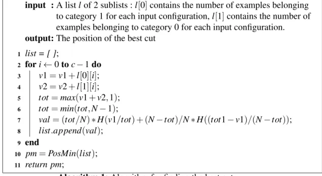
The observation, we made previously, leads us to choose information instead of pro-bability in the greedy initialization. More specifically, we worked with the average en-tropy of the error rate. First, we count how many examples that produce this input for this gate belong to each category (i.e., as done when maximizing probability) and then we sort them in decreasing order according to one of the two categories (i.e. we chose category 1). Second we will try to divide input configurations according to the average entropy into two groups, one group will be assigned category 1 and the other one will be assigned category 0. In other terms, we will look for the best cut (i.e., the best posi-tion) where the average entropy calculated for category 1 is minimal then the first input
configurations will be given 1 in the truth table whereas the rest will be given 0. The algorithm describing steps for searching the best cut is shown below.
Table 4.VII and table 4.VIII illustrate an example of applying the algorithm for sear-ching the best cut. Table 4.VIII represents the second step where the table is sorted in a decreasing order. Then using the formula described in the algorithm below, the best cut will be as follows : the first three lines belong to category 1 whereas the last one belongs to category 0, the cut is shown by a bold horizontal line in the table 4.VIII. Therefore the truth table of such gate will be [1, 0, 1, 1].
Let tot1 be the total of examples belonging to category 1, N the total of examples, c the number of configuration of the inputs (e.g., 4 for a 2-gate) and the function H(x) is the function calculating the entropy of variable x.
input : A list l of 2 sublists : l[0] contains the number of examples belonging to category 1 for each input configuration, l[1] contains the number of examples belonging to category 0 for each input configuration.
output: The position of the best cut
1 list = [ ]; 2 for i ← 0 to c − 1 do 3 v1 = v1 + l[0][i]; 4 v2 = v2 + l[1][i]; 5 tot= max(v1 + v2, 1); 6 tot= min(tot, N − 1);
7 val= (tot/N) ∗ H(v1/tot) + (N − tot)/N ∗ H((tot1 − v1)/(N − tot)); 8 list.append(val);
9 end
10 pm= PosMin(list); 11 return pm;