HAL Id: hal-01625736
https://hal.archives-ouvertes.fr/hal-01625736
Submitted on 1 Nov 2017
HAL is a multi-disciplinary open access
archive for the deposit and dissemination of
sci-entific research documents, whether they are
pub-lished or not. The documents may come from
teaching and research institutions in France or
L’archive ouverte pluridisciplinaire HAL, est
destinée au dépôt et à la diffusion de documents
scientifiques de niveau recherche, publiés ou non,
émanant des établissements d’enseignement et de
recherche français ou étrangers, des laboratoires
Experimental comparisons between implicit and explicit
implementations of discrete-time sliding mode
controllers: Towards chattering suppression in output
and input signals
Bin Wang, Bernard Brogliato, Vincent Acary, Ahcene Boubakir, Franck
Plestan
To cite this version:
Bin Wang, Bernard Brogliato, Vincent Acary, Ahcene Boubakir, Franck Plestan. Experimental
com-parisons between implicit and explicit implementations of discrete-time sliding mode controllers:
To-wards chattering suppression in output and input signals. VSS 2014 - 13th IEEE International
Work-shop on Variable Structure Systems, Jun 2014, Nantes, France. pp.1-6, �10.1109/VSS.2014.6881159�.
�hal-01625736�
Experimental comparisons between implicit and explicit
implementations of discrete-time sliding mode controllers: towards
chattering suppression in output and input signals
B. Wang, B. Brogliato, V. Acary, A. Boubakir, F. Plestan
Abstract— This paper presents a set of experimental results concerning the sliding mode control of an electro-pneumatic system. Two discrete-time control strategies are considered for the implementation of the discontinuous part of the sliding mode controller: explicit and implicit discretizations. While the explicit implementation is known to generate numerical chattering [6], [7], [12], [13], the implicit one is expected to significantly reduce chattering while keeping the accuracy. The experimental results reported in this work remarkably confirm that the implicit discrete-time sliding mode supersedes the explicit ones, with several important features: chattering in the control input is almost eliminated (while the explicit and saturated controllers behave like high-frequency bang-bang inputs), the input magnitude depends only on the perturbation size and is largely independent of the controller gain and sampling time.
I. INTRODUCTION
Consider the scalar system ˙x(t) = u(t)+d(t), with u(t) ∈ −sgn(x(t)), where sgn(·) is the set-valued signum function: sgn(0) = [−1, 1], sgn(x) = 1 if x > 0, sgn(x) = −1 if x < 0. Let the disturbance d(t) satisfy |d(t)| ≤ δ < 1 for some δ. Using Filippov’s mathematical framework of differential inclusions, one deduces that for any x(0), the state x(t) reaches the “sliding surface” x = 0 in a finite time t∗, and then x(t) = 0 for all t ≥ t∗. In the differential
inclusions language, u(t) is a selection ξ(t) of the interval [−1, 1] for t ≥ t∗, and it satisfies ξ(t) = u(t) = −d(t) after
t∗. In a sense, the set-valued controller acts as a disturbance
observer once the sliding mode is attained. It is clear that if one multiplies the signum by a gain a > 0, i.e. u(t) = a sgn(x(t)), then one still has u(t) = −d(t) in the sliding phase after t∗. However this time the value of the selection
ξ(t) inside the set-valued part of sgn(x(t)) is divided by a, i.e.ξ(t) = d(t)a .
Let us now consider the Euler discretization of this system. It reads: xk+1 = xk+ huk+ hdk, where fk = f (tk) for a
Bin Wang was with BIPOP team, INRIA Grenoble, 655 avenue de l’Europe, 38334 Saint-ismier, France.
Bernard Brogliato is with BIPOP team, INRIA Grenoble, 655 avenue de l’Europe, 38334 Saint-ismier, France. [email protected]
Vincent Acary is with BIPOP team, INRIA Grenoble, 655 avenue de l’Europe, 38334 Saint-ismier, France. [email protected]
Ahcene Boubakir is with Laboratoire de Commande des Processus, Ecole Nationale Polytechnique d’Alger, Alg´eria. This work was perfomed during a stay at IRCCyN, Nantes, France. ah [email protected]
Franck Plestan is with IRCCYN, Ecole Centrale de Nantes, 1 rue de la No¨e, BP 92101, 44321 Nantes Cedex 3, France. [email protected]
This work has been performed with the support of the French National Research Agency (ANR) project ChaSliM (ANR 2011 BS03 007 01).
function f(·), and tk = t0+kh are the sampling times, h > 0
is the sampling period. In such a simple case, the Euler and ZOH discretizations are the same, except for the disturbance dk=!
tk+1
tk d(t)dt for the ZOH method. Our focus is on how
to choose uk. The explicit method yields uk ∈ −sgn(xk),
yielding the closed-loop xk+1− xk− hdk∈ −h sgn(xk). As
alluded to above, limit cycles exist which create oscillations around the sliding surface (here the origin), known as the numerical chattering in the output [6], [7], [12], [13]. One of the consequences is that the explicit controller keeps switching between the two values 1 and -1, and never attains any point inside (−1, 1). In particular the explicit controller cannot approximate the continuous-time selection ξ(·) = u(·) when the system evolves close to the sliding surface. If a gain a >0 premultiplies u(·) then the explicit controller switches between two discrete values a and −a, the switching frequency being inversely proportional to the sampling period: this is the numerical chattering in the input. It is noteworthy that the mere notion of a sliding surface does not exist in this case, since the discrete trajectories cannot attain the origin, and the controller cannot take values in the set-valued part equal to (−1, 1). One then has to resort to so-called quasi-sliding surfaces [3], [11].
The implicit method is implemented as follows. Since d(t) is unknown, one first constructs a nominal unperturbed system with state x˜k, from which the input is computed:
˜
xk+1 = xk + huk, uk ∈ −sgn(˜xk+1). This is a so-called
generalized equationwith unknown˜xk+1. Its solution yields
after few manipulations uk= h proj
"
[−1, 1]; −xk h
#
that is the projection on the interval[−1, 1], and is a causal input (not depending on future values of the state). Notice that in the unperturbed case, x˜k and xk are the same.
As proved in [1], [2], the implicit controller guarantees convergence ofx˜k to the origin in a finite number of steps,
and disturbance attenuation by a factor h during the sliding mode. Most importantly, the control input takes values in (−1, 1) once ˜xkhas reached the origin, as may be seen from
the generalized equation from which it is calculated, and one has during that phase uk = −dk: uk is a selection ξk of
the discrete-time differential inclusion x˜k+1 = xk + huk,
uk ∈ −sgn(˜xk+1), and the discrete-time input observes the
disturbance when the sliding mode is attained. Similarly to the continuous-time case, if the controller is multiplied by a
gain a >0, then the selection ξk = −dak.
Therefore the implicit controller has the same features as its continuous-time counterpart. We may summarize them as follows:
(i) When there is no perturbation, the sliding surface is reached after a finite number of steps. When a perturba-tion acts on the system, the state of the nominal system reaches the sliding surface after a finite number of steps, while the perturbation effect is attenuated by a factor h on the system’s state.
(ii) Despite the system’s state xk never attains its sliding
surface due to the disturbance, the notion of discrete-time sliding mode does exist, and corresponds to the nominal system’s state x˜k vanishing, or equivalently
to the set-valued controller evolving strictly inside the interval[−1, 1]. In this mode the controller compensates for the disturbance, and is a copy of it. Its magnitude is therefore independent, in the sliding mode, of the controller gain, and there is no need to adapt the gain (denoted as a above, and as G in the sequel) on-line. (iii) Theoretically there is no numerical chattering during the
sliding mode, neither in the sliding variable, nor in the input.
(iv) The discrete-time controller keeps the simplicity of its continuous-time counterpart, with no added gain to tune. (v) Computing the input at each step boils down to solving a simple generalized equation, equivalently a projection on[−1, 1], or solving a quadratic program. This is quite easy to implement in a code.
The implicit algorithm extends to higher dimension systems, and with sliding surfaces of codimension ≥ 2 [2]. The main objective of this note is to confirm these features experimentally.
II. DYNAMICS OF THE PLANT AND CONTROLLERS
The electropneumatic system used for the controllers eval-uation consists in two actuators which are controlled by two servodistributors (see Figure 1).
Fig. 1: [10] the electropneumatic system - On the left hand side is the “main” actuator whose its position is controlled. On the right hand side is the “perturbation” actuator whose load force is controlled.
Under some assumptions detailed in [10], the dynamic model
of the pneumatic actuator can be written as a nonlinear system which is affine in the control input [uP uN]
T
, uP
(resp. uN) being the control input of the servodistributor
connected to the P (resp. N ) chamber. The model is divided in two parts: two first equations concern the pressure dynam-ics in each chamber whereas the motion of the actuator is described by the two last equations. Then the model of the electropneumatic experimental set-up reads as
⎧ ⎪ ⎪ ⎪ ⎪ ⎪ ⎪ ⎪ ⎪ ⎪ ⎨ ⎪ ⎪ ⎪ ⎪ ⎪ ⎪ ⎪ ⎪ ⎪ ⎩ ˙pP = krT VP(y) [ϕP+ ψP· uP− S rTpPv] ˙pN = krT VN(y) [ϕN+ ψN· uN+ S rTpNv] ˙v = 1 M[S (pP− pN) − bvv− F ] ˙y = v, (1)
with pP (reps. pN) the pressure in the P (resp. N ) chamber,
y and v being the position and velocity of the actuator. The force F is a disturbance. Note that the previous system appears to have two control inputs given that there is one servo distributor connected to each chamber. In the sequel, only the main actuator position is controlled: given that there is a single control objective, one states
u= uP= −uN.
The choice of sliding mode controller has been made because of its intrinsic features of robustness. Let us define the so-called sliding variable as
σ(x, t) = ¨e+ λ1˙e + λ0e (2)
with e = y − yd(t), yd(t) being the desired trajectory,
supposed to be sufficiently differentiable. As shown in [9], [8], the first time derivative of σ can be written as
˙σ = Ψ(x, t) + Φ(x)u
= Ψn(x, t) + ∆Ψ(t) + [Φn(x) + ∆Φ(t)] u (3)
such that Ψn,Φn are the nominal functions and ∆Ψ, ∆Φ
are the uncertain terms. From [9], [8], functions Ψ and Φ are bounded in the physical working domain (which gives that the uncertain terms are also bounded). Furthermore, one supposes that ∆Φ is sufficiently small with respect to Φn
to ensure that1 +∆ΦΦn >0. From a practical point of view,
this assumption is not too strong: it simply means that the uncertainties are small compared to the nominal values. Let us consider the control law1:
u = 1 Φn
[−Ψn+ v] . (4)
By applying (4) in (3), one gets ˙σ = ∆Φ Φn Ψn+ ∆Ψ + ( 1 +∆Φ Φn ) v. (5)
1As shown in [4], such a control law allows to reduce the magnitude
of the sliding mode controller by using the nominal informations in the controller.
Once u has been designed to linearize by feedback the system (1), the discontinuous part of the controller is defined as
v ∈ −Gsgn(σ) (6) with G tuned sufficiently large. The controller v has been implemented under its discrete forms as follows (with k≥ 0, σk= σ(kh), h being the sampling period)
• Explicit sliding mode control (with sgn(·) function)
vk = −Gsgn(σk), (7) • Implicit sliding mode control (with sgn(·)
multifunc-tion)
vk ∈ −Gsgn(σk+1) (8)
(implemented with a projection as indicated in the introduction).
III. EXPERIMENTAL RESULTS
The two controllers have been implemented with several feedback gains and sampling times. The length of the interval of study is 20 seconds. The comparisons are made mainly with respect to: the input v magnitude and chattering, and the tracking error.
A. Comparison of the tracking errorse
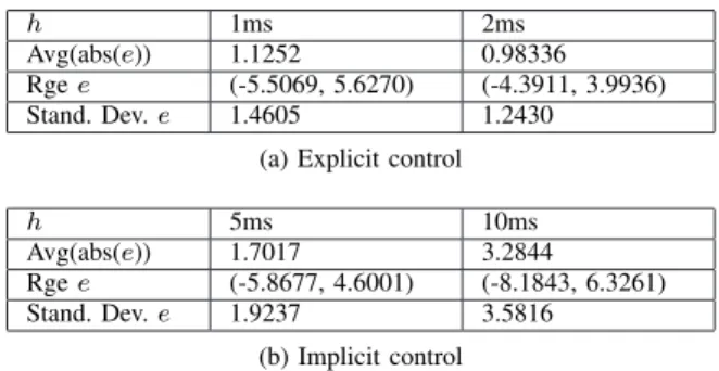
Data in Tables I–II and III–V characterize the position tracking error e obtained by the two different implementa-tion methods, from the aspects of average, range, standard deviation and variation with five different sampling periods. The symbol Avg denotes the average of the tracking error over the duration of the test, abs is the absolute value of tracking error, Rge is the range. The variation of a real-valued function f(·) defined on an interval [a, b] ⊂ R is the quantity V ar[a,b](f ) = N −1 * i=0 |f (ti+1) − f (ti)| (9)
where the set of time instants {t0, t1,· · · , tN} is a partition
of[a, b]. In the following, the variations of the position error e for the two implementation methods with the different gains G, have been calculated by choosing the partition times ti
in (9), as the sampling times.
Remark 3.1: The variation in (9) as a quantity to char-acterize the analyzed signals, is not common in Control Engineering. It is thought here in the context of sliding mode control, that such a quantity is useful to measure the chattering level of a signal, since it does represent how much the signal varies. However due to the partition that has been chosen (the sampling times) the results are not comparable from one sampling period to the next, but only between the three controllers for a fixed h. In other words, in Tables III— V data have to be compared inside a single column, but not from one column to another one.
All the data concerning e are reported in Tables I—V and Figure 2. It is confirmed in Tables III–V, that the variation of the implicit input starts to be significantly smaller than that of
the other two, for h≥ 5 ms, the improvement being huge for h= 15 ms. These first data tend to indicate that, in the case of the implicit input, its variation is drastically smaller for larger sampling periods (for h= 15 ms: 1836 for the explicit method,8.10 for the implicit one with G = 104), confirming
that chattering on e is reduced when the implicit controller (8) is used. The fact that the output signal is smooth for the implicit method, while it chatters for the explicit controller for large sampling time, is obvious in Figure 2. Similar conclusions were obtained for G= 104 and are not reported
here because of lack of space.
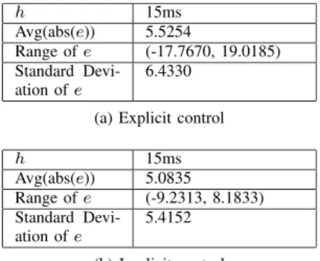
Tables I—II concerns G= 105. The two methods show
similar results in terms of average, range and standard deviation of e, the implicit one providing slightly better results. The variation values are given in Tables III—V with G= 105, and is quite visible in Figure 2: the variation of e
with the implicit input is much smaller than with the explicit controllers, except for h= 1 ms where the obtained values are of same order. This indicates that the chattering on e is drastically reduced with the implicit input2.
! A first conclusion, that will be strengthened in the next paragraph, is that the implicit control method allows to take larger gains without decreasing the performance (it means that it is possible to reject/counteract larger pertur-bations/uncertainties without more chattering). The perfor-mance of implicit control is better whenG is larger, while it is less good with the explicit and saturation controllers.
h 1ms 2ms
Avg(abs(e)) 1.1252 0.98336
Rge e (-5.5069, 5.6270) (-4.3911, 3.9936)
Stand. Dev. e 1.4605 1.2430
(a) Explicit control
h 5ms 10ms
Avg(abs(e)) 1.7017 3.2844
Rge e (-5.8677, 4.6001) (-8.1843, 6.3261)
Stand. Dev. e 1.9237 3.5816
(b) Implicit control
TABLE I: Comparisons of position error e when G= 105.
2The results for too small sampling periods (h ≤ 2 ms) are not
conclusive, because of the limited bandwidth of the filters used to compute ˙e and ¨e to construct σ.
h 15ms Avg(abs(e)) 5.5254 Range of e (-17.7670, 19.0185) Standard Devi-ation of e 6.4330 (a) Explicit control
h 15ms Avg(abs(e)) 5.0835 Range of e (-9.2313, 8.1833) Standard Devi-ation of e 5.4152 (b) Implicit control
TABLE II: Comparisons of position error e when G= 105.
h 1ms 2ms
Explicit control 3.7426e+03 2.5724e+03 3
Implicit control 3.1577e+03 1.6360e+03
(a) G= 105
TABLE III: Variation of position error e.
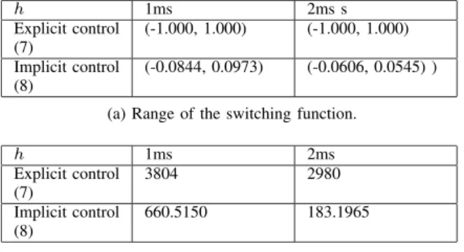
B. Comparison of discontinuous inputsv in (7) and (8): The features of the control inputs is a key-point in this work, given that one of the objectives is to show the influence of implicit control to the chattering effect. Let us now pass to the control inputs comparisons, with data reported in Tables VI–VIII, Tables IX–XI and Figure 3. Data given in Tables VI–VIII and IX–XI characterize the “switching functions” for these three methods. It includes the range and variation. Remark 3.1 applies also for the variation of the control, so that in Tables VI–VIII, data have to be compared inside a single column, but not from one column to another one.
! What we call the switching functions are sgn(σk) in
(7), and sgn(σk+1) in (8). For the implicit controller, this is
what we called the selectionξk in Introduction. This is not
to be confused with the discontinuous controlv in (6). Comparisons of the inputs in the two methods are given in Tables VI–VIII from range and variation aspects. In addition, the two controllers are depicted in Figure 3, for various time steps and gains.
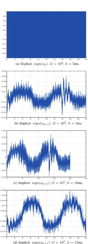
Globally, the experimental results show that the implicit method drastically reduces the input chattering and mag-nitude compared with the explicit method. The explicit switching input keeps oscillating between the maximum and minimum values like a bang-bang controller (see data in Tables VI–VIII, and Figure 3(a), which is quite representative of all the switching functions obtained with explicit dis-cretizations). In the tables, all the values used to characterize the chattering in implicit method are invariably much less than the explicit method. Figures 3(b)–3(d), which concerns the implicit controller switching function for various sam-pling times, show that the implicit input v in (8) is largely independent sampling time. From Table VI–VIII, the data in the rows corresponding to the implicit controller allow to obtain a confirmation of this fact. The magnitudes of the switching function for the implicit controller, for 6 different gains G and two different sampling periods h, are reported in
h 5ms 10ms s
Explicit control 1.7742e+03 1.6081e+03
Implicit control 650.2710 480.1660
(a) G= 105
TABLE IV: Variation of position error e.
h 15ms
Explicit control 2.5070e+03
Implicit control 228.8022
(a) G= 105
TABLE V: Variation of position error e.
Tables IX–XI. It confirms that the magnitude of the input v in (6), which is the switching function times the gain G, does not depend neither on G nor on h in this range of sampling times.
! This insensitivity property is believed to be a funda-mental property of the implicit method introduced in [1], [2], compared to explicit implementations which drastically differ whenh and/or G are varied.
The results depicted in Figure 3 clearly demonstrate that whereas the explicit controller tends to approximate a signal that switches infinitely fast between two extreme values like bang-bang inputs, this is not at all the case for the implicit controller that behaves in a totally different way. This is a nice confirmation of both theoretical and numerical predictions [1], [2], that the implicit controller does repre-sent the discrete-time approximation of the selection of the differential inclusion according to Filippov’s mathematical framework.
Input chattering is also visible in Table VI–VIII. Variation of the implicit switching function is much smaller than the other two.
C. Summary
These extensive experimental tests prove that items (ii) (iii) (iv) and (v) in the Introduction, are not only theo-retical and numerical predictions obtained in [1], [2], but significantly influence the discrete-time implemented sliding-mode controller. The implicit method (8) allows to drastically reduce the input chattering and magnitude, while enhancing the tracking capabilities (output chattering is almost entirely eliminated). It also allows the designer to choose larger sampling periods, which may be of strong interest in practice. Perhaps counter-intuitively for Control Engineers, the perfor-mance and robustness increase when the gain G increases, which is thought to considerably simplify the controller gain tuning process.
We have also conducted extensive experiments with a saturated explicit input. The results we obtained are quite similar to the case without saturation (the saturation seems to play a very tiny role in chattering effects), and are therefore not reported in this note.
h 1ms 2ms s Explicit control (7) (-1.000, 1.000) (-1.000, 1.000) Implicit control (8) (-0.0844, 0.0973) (-0.0606, 0.0545) ) (a) Range of the switching function.
h 1ms 2ms Explicit control (7) 3804 2980 Implicit control (8) 660.5150 183.1965
(b) Variation of the switching function.
TABLE VI: Switching function, gain G= 105.
h 5ms 10ms Explicit control (7) (-1.000, 1.000) (-1.000, 1.000) Implicit control (8) (-0.0360, 0.0417) (-0.0289, 0.0349) (a) Range of the switching function.
h 5ms 10ms Explicit control (7) 2050 1932 Implicit control (8) 34.7510 25.2005
(b) Variation of the switching function.
TABLE VII: Switching function, gain G= 105.
IV. CONCLUSION
Experiments have been conducted on an electropneumatic system, with two different implementations of the sliding mode controller: explicit and implicit discretizations. The results demonstrate that the theoretical and numerical pre-dictions of [1], [2] are true: the implicit implementation, which consists merely of a projection on the interval[−1, 1] and is thus very easy to implement in a code, drastically supersedes the other one. The output and input chattering are reduced in a significant way, without changing the controller basic structure (i.e., no additional filter, observer, or dynamic controller is added compared to the original, basic sliding mode controller) and keeping its simplicity (in particular the gain tuning is easy, which is a strong feature of the ECB-SMC method). The main feature of the implicit discretization, is that it keeps, in discrete-time, the multivalued feature of the theoretical continuous-time sliding-mode controller, as it is mathematically imposed in Filippov’s framework. The proposed implicit discretization method is generic in the sense that it could apply to any kind of sliding mode, set valued control. Future research should therefore concern similar experiments on the same and other set-up, with twisting and high-order sliding-mode controllers.
h 15ms
Explicit control (7) (-1.000, 1.000)
Implicit control (8) (-0.0173, 0.0247)
(a) Range of the switching function.
h 15ms
Explicit control (7) 1836
Implicit control (8) 8.1039
(b) Variation of the switching function.
TABLE VIII: Switching function, gain G= 105.
G 104 5.104
h= 5 ms (−0.3, 0.35) (−0.05, 0.05)
h= 10 ms (−0.25, 0.3) (−0.05, 0.06)
TABLE IX: Magnitude of implicit switching function sgn(xk+1) for varying gains G and sampling period h.
REFERENCES
[1] V. ACARY, B. BROGLIATO, Implicit Euler numerical scheme and chattering-free implementation of sliding mode systems, Systems and Control Letters, vol.59, pp.284-293, 2010.
[2] V. ACARY, B. BROGLIATO, Y. ORLOV, Chattering-free digital sliding-mode control with state observer and disturbance rejection, IEEE Trans. Automatic Control, vol.57, no 5, pp.1087-1101, May 2012.
[3] BARTOSZEWICZ, A , Discrete-time quasi-sliding-mode control strate-gies, IEEE Transactions on Industrial Electronics, vol. 45, no 4, pp. 633–637, 1998.
[4] R. CASTRO-LINARES` , S. LAGHROUCHE, A. GLUMINEAU, ANDF. PLESTAN, Higher order sliding mode observer-based control, IFAC Symposium on System, Structure and Control, Oaxaca, Mexico, 2004. [5] L. FRIDMAN, J. MORENO ANDR. IRIARTE(EDITORS), Sliding Modes after the First Decade of the 21st Century. State of the Art, Lecture Notes in Control and Information Sciences, Volume 412, 2012, DOI: 10.1007/978-3-642-22164-4 , Springer Verlag Berlin Heidelberg. [6] Z. GALIAS, X. YU, Complex discretization behaviours of a
sim-ple sliding-mode control system, IEEE Transactions on Circuits and Systems–II: Express Briefs, vol.53, no 8, pp.652-656, August 2006. [7] Z. GALIAS, X. YU, Analysis of zero-order holder discretization of
two-dimensional sliding-mode control systems, IEEE Transactions on Circuits and Systems–II: Express Briefs, vol.55, no 12, pp.1269-1273, December 2008.
[8] A. GIRIN, F. PLESTAN, X. BRUN, AND A. GLUMINEAU, Robust control of an electropneumatic actuator : application to an aeronautical benchmark, IEEE Transactions on Control Systems Technology, vol.17, no.3, pp.633-645, 2009.
[9] S. LAGHROUCHE, M. SMAOUI, F. PLESTAN,ANDX. BRUN, Higher order sliding mode control based on optimal approach of an elec-tropneumatic actuator, International Journal of Control, vol.79, no.2, pp.119-131, 2006.
[10] Y. SHTESSEL, M. TALEB,ANDF. PLESTAN, A novel adaptive-gain supertwisting sliding mode controller: methodology and application, Automatica, vol.48, no.5, pp. 759-769, 2012.
[11] SIRA–RAMIREZ, H., Non–linear discrete variable structure systems in quasi–sliding mode, Int, J. Control, vol.54, no.5, pp. 1171–1187, 1991.
[12] B. WANG, X. YU, G. CHEN, ZOH discretization effect on single-input sliding mode control systems with matched uncertainties, Automatica, vol.45, pp.118-125, 2009.
[13] X. YU, B. WANG, Z. GALIAS, G. CHEN, Discretization effect on equivalent control-based multi-input sliding-mode control systems, IEEE Transactions on Automatic Control, vol.53, no 6, pp.1563-1569, July 2008.
G 105 5.105
h= 5 ms (−0.03, 0.035) (−0.006, 0.0063)
h= 10 ms (−0.025, 0.03) (−0.005, 0.006)
TABLE X: Magnitude of implicit switching function sgn(xk+1) for varying gains G and sampling period h.
G 106 5.106
h= 5 ms (−0.003, 0.003) (−0.0006, 0.00065)
h= 10 ms (−0.0025, 0.0025) (−0.0005, 0.0005)
TABLE XI: Magnitude of implicit switching function sgn(xk+1) for varying gains G and sampling period h.
0 2 4 6 8 10 12 14 16 18 20 −50 −40 −30 −20 −10 0 10 20 30 40 50
(a) h= 1ms. Explicit method.
0 2 4 6 8 10 12 14 16 18 20 −50 −40 −30 −20 −10 0 10 20 30 40 50 (b) h= 1ms. Implicit method. 0 2 4 6 8 10 12 14 16 18 20 −60 −40 −20 0 20 40 60 (c) h= 15ms. Explicit method. 0 2 4 6 8 10 12 14 16 18 20 −40 −30 −20 −10 0 10 20 30 40 (d) h= 15ms. Implicit method.
Fig. 2: Real position y (mm) in blue and yd (mm) in red,
under h= 1ms and h = 15ms for G = 105.
0 2 4 6 8 10 12 14 16 18 20 −1 −0.8 −0.6 −0.4 −0.2 0 0.2 0.4 0.6 0.8 1
(a) Explicit. sign(sk). G = 104, h= 5ms.
0 2 4 6 8 10 12 14 16 18 20 −0.04 −0.03 −0.02 −0.01 0 0.01 0.02 0.03 0.04 0.05 (b) Implicit. sign(sk+1). G = 105, h= 5ms. 0 5 10 15 20 25 −0.03 −0.02 −0.01 0 0.01 0.02 0.03 0.04 (c) Implicit. sign(sk+1). G = 105, h= 10ms. 0 2 4 6 8 10 12 14 16 18 20 −0.02 0.015 −0.01 0.005 0 0.005 0.01 0.015 0.02 0.025 (d) Implicit. sign(sk+1). G = 105, h= 15ms.
Fig. 3: Switching function: Comparison between explicit method (sign(sk)) and implicit method (sign(sk+1)).
![Fig. 1: [10] the electropneumatic system - On the left hand side is the “main” actuator whose its position is controlled.](https://thumb-eu.123doks.com/thumbv2/123doknet/11362219.285446/3.892.497.837.237.377/fig-electropneumatic-left-hand-main-actuator-position-controlled.webp)